1. Introduction
Bad traffic is experienced in most cities of developing countries. A current traffic problem, which is getting worse every day, is the increase in travel times (see the congestion levels in [
1]). Thus, gaining insight into situations inducing higher travel times is of utter importance. One of those situations is when drivers, intentionally or owing to the operating limitations of the vehicle they drive, travel at a lesser speed than the posted speed limit. Therefore, in the same stretch of road, the drivers’ desired speed (or speed tendency) may vary and there is a likely chance of slow vehicles impeding fast vehicles. The traffic outcome when fast and slow vehicles interact is difficult to establish and is related with the drivers’ desired speed and the percentage of slow vehicles, among other variables.
The aim of the present research is, firstly, to perform simulations with different percentages of fast and slow vehicles for proposed values for each speed tendency. The output of these simulations is the mean extra travel time (T) and the extra travel time variability (V) of the fast vehicles. These data (i.e., T and V) are divided into two groups: the data for modeling and the data for validating. Later, procedures for modeling T and V are proposed with the intention to prove if the patterns in the data (for modeling) can be reproduced. In addition, we demonstrate that the data for validating can be explained with the proposed models, and we present how to calculate the models’ parameter values as part of the procedures.
In a traffic scenario with vehicles driving slower than the general traffic stream (thus generating a speed differential), when the faster vehicles are impeded by the slower vehicles, the former are tempted to perform overtaking maneuvers, if possible. In [
2], it was proven that the vehicles’ travel speed (and thus also travel time) is affected, among others, by the traffic composition in terms of speeds. In [
3], a relationship between speed variance and accidents was established, finding that an increase in average speed does not necessarily increase accident rates, but an increase in speed variance certainly increases them. In [
4], the proposed algorithm triggers a need to overtake when the speed differential is 8 km/h. The work in [
5] focuses on establishing (via simulations) the average travel time to complete a highway segment and the number of passenger cars’ lane changes with different percentages of heavy trucks. The results show that both variables increase as the percentage of heavy trucks increases, with the influence of heavy trucks on traffic being notorious in heavy traffic. In [
6], speed indicators on sites with uniform speed limits (65 mph for passenger vehicles and trucks/buses) and with differential speed limits (70 mph for passenger vehicles and 60 mph for trucks/buses) were investigated. The results from the models were a mean speed of 65.3 mph for the uniform case (one) and 66.9 mph for the differential case (two). Similarly, the 85th percentile speed results were 70.7 mph for case one and 73.9 mph for case two. Finally, the standard deviation was 5.5 mph for case one and 6.8 mph for case two. Through simulations, the impact on traffic of differential speed controls was investigated in [
7]. The speed control strategies were uniform posted speed limits (USLs), differential posted car–truck speed limits (DSLs), and differential mandated truck speed limits (MSLs). Considered positive for traffic safety, DSL and MSL reduce average travel speed, increase head-on time-to-collision, and reduce car–car overtaking. Considered negative, DSL and MSL increase percentage time spent following and total number of overtakes, decrease car–car overtaking, but increase car–truck overtaking. In [
8], considering all types of vehicles, it was detected that the highest travel speed variability occur in freeways with DSL, followed by urban freeways with USL and a speed limit of 55 mph. For passenger cars, the speed was consistent when the speed limit was 70 mph, but at lower speed limits, more speed variation was detected.
Different factors are related to free-flow speed; one of those is differential speed. In [
9], the free-flow speed was modeled considering as an explanatory variable the trucks’ percentage in order to test if the flow heterogeneity (the traffic composition in terms of vehicles’ type) impacted speed. The results showed that the trucks’ percentage is significant for the four models: daytime speed for cars and trucks, and nighttime for cars and trucks. In [
10], with the aim of identifying explanatory factors for mean speed and speed dispersion considering two-lane rural highways on tangent segments and horizontal curves, free-flow speed models were developed.
The drivers’ travel speed is influenced by the posted speed limit. In [
11], it was found that the posted speed limit is highly correlated with the average free-flow speed for urban streets, multilane highways, and freeways. In [
12], the speed limits in Utah rural interstates were increased from 75 to 80 mph, finding that the travel speed and the probability to overcome the speed limit were then higher, and that by increasing the speed limit, the speed variance was not reduced. However, as the literature review presented in [
13] suggests, the results concerning the effects of speed limit on speed variation do not support each other. The investigation in [
14] centers on the local and global impacts of speed limits considering two groups of drivers—the compliant and the non-compliant drivers. When choosing speed, both consider the travel time cost, the perceived crash risk, and the perceived ticket risk.
The factors influencing the drivers’ desired speed on the road are numerous. There are multiple interacting factors that explain drivers’ behaviors [
15]. A study on drivers’ speeding behavior is presented in [
16]. The drivers’ characteristics and their relation to speed (as a risk of accidents level) are presented in [
17]. In [
18], the drivers’ speed choice (when there is at least a 6 s time gap to the next vehicle) at two different sites were compared, and at two different days for the same site. How a driver is influenced by the collective driving behavior is discussed in [
19]. Empirical evidence suggesting that the speed choice is influenced by the pleasure of driving and other drivers’ behavior is presented in [
20]. Preliminary data for supporting the notion that a driver adjusts their speed by comparing their own speed with that of others are introduced in [
21]. A model including attitudes and perceptions of other drivers’ behavior explains approximately 15% of the variation in observed speed [
22]. A speed choice prediction model was presented in [
23]. It was found that the number of heavy vehicles (trucks and buses) and four-wheelers (informal para-transit) flowing in the same direction as the subject vehicle negatively influences the driver speed choice of the higher-speed class, and the same applies for trucks and motorcycles driving in the opposite direction. Buses, trucks, four-wheelers, and motorcycles negatively influence the speed of the lower-speed class (same traffic direction), and the same applies for non-motorized and buses driving in the opposite direction. The operating speed was modeled in [
24], and the dependence of the drivers’ speed choice on individual driver’ behavior and the roadway geometry was demonstrated.
The necessity of vehicle class-specific modeling has been noted. Models to establish the free-flow speed of different types of vehicles are presented in [
25]. In [
26], it was found that the level-of-service (LOS) is different for each vehicle type. Besides, removing some vehicle types seems suitable to improve the system performance. Further, it was noticed that, in mixed traffic, the average stream speed better represents the dominant vehicle type, which is two-wheelers in [
26]. The work in [
27] uses percent speed-reduction and percent slower vehicles to define the LOS of a two-lane highway under heterogeneous traffic. It was concluded that it is impractical to evaluate the LOS of the entire traffic situation (with integration of motorized and non-motorized modes) with a common scale. In [
28], two new methodologies are presented for estimating the percent time spent following (PTFS) on two-lane highways. The probabilistic method considers the slow-moving vehicles’ average speed and the distribution of the desired speeds to calculate the percentage of vehicles whose desired speed is superior to the slower vehicles’ average speed. This percentage (used to calculate the probability of a vehicle being impeded), along with the probability of a vehicle being part of a platoon, are used to calculate the percent following (PF), which is a surrogate measure for PTFS. In [
29], it was noticed that the aggregation of faster and slower vehicles on a single class may not capture the interactions among the vehicles of the same class.
The dynamic of homogeneous and heterogeneous traffic is very different; in the latter, there are different types of vehicles, thus there are interactions (such as lane change maneuvers) between slow-moving and fast-moving vehicles. In [
30], particle-hopping models for two-lane traffic were developed considering two types of vehicles: fast and slow vehicles, where the fast vehicles’ maximum allowed speed is considerable higher than that of the slow vehicles. The proposed models are different from each other because of the lane-changing rules, thus producing different results about the movement of the fast and slow vehicles. In [
31], the heterogeneous traffic behavior in developing countries was reproduced with a discrete cellular automata (CA) model, modeling five types of vehicles: car, bus, truck, two-wheeler, and three-wheeler. In [
32], a CA model was used to simulate traffic in a two-lane system; it was demonstrated that even small densities of slow vehicles induced the formation of platoons. Moreover, modifications were incorporated into the basic model, e.g., for allowing drivers to anticipate the speed of their predecessor, leading to diminishing the effect of slow vehicles. The multi-class traffic flow model presented in [
33] incorporates heterogeneous drivers, i.e., drivers selecting a different speed to drive, thus there are faster vehicles trying to overtake slower vehicles. In addition, the model explains traffic flow theory phenomena: two-capacity regimes in the fundamental diagram, hysteresis, and platoon dispersion. In [
34], a vehicle class was defined considering the desired speed in free-flow conditions, and a multiclass first-order simulation model was proposed that can replicate non-linear phenomena, including the dispersion of traffic platoons when a distribution of desired speeds exists. In [
35], data were collected in several two-lane roads in India, and it was observed that the capacity decreases as the proportion of three-wheeler, tractor, or heavy vehicle increases, and that the capacity increases as the proportion of two-wheeler increases. In [
36], through agent-based modeling, simulations representative of the traffic in the USA (with cars and trucks) and of the traffic in India (with different types of vehicles) were performed. It was found that the heterogeneity of vehicle types causes a high number of lane changes.
In this investigation, we simulate and analyze traffic, where the speed differential affects travel speed, thus affecting travel time. We were interested in finding a relation between the percentage of slow vehicles and two variables related with the fast vehicles: the mean extra travel time (T) and the extra travel time variability (V). We propose procedures for modeling two metrics of importance in traffic studies: T and V, which were calculated with the fast vehicles’ travel times from simulations. Our research is different from the current literature as we perform traffic simulations considering a wide range of fast and slow vehicles’ percentage values for a wide range of fast and slow vehicles’ speed tendency values, thus adding insight for this kind of traffic situation. Our proposed procedures have the advantage of including a method for calculating the parameters’ values of the models that describe the data (T and V) that were not used to calibrate the models. In this research, we have two general objectives:
- (1)
For each fast vehicles’ speed tendency (sp1) value, to run a simulation for each slow vehicles’ percentage (p2) value, in order to acquire traffic information (the fast vehicles’ travel times) and calculate the mean extra travel time and the extra travel time variability. The data, i.e., T and V are divided in two groups: 1. the data for modeling and 2. the data for validating.
- (2)
Establish procedures for modeling the first group of data and for explaining the second group of data. Calculate the models’ error and identify the procedures reporting the lower mean error, i.e., the suitable proposals to describe the T and V patterns.
4. Discussion
4.1. Discussion for Explaining T
Table 26 presents the error (obtained in procedure 1, 2, and 3) between a vector with data for modeling (
) and the directly modeled vector (
). It also shows the mean of the errors
for
cases {60,65,75,85,90}, i.e.,
. The lower mean error is presented by procedure 1, followed closely by procedure 3.
Similarly,
Table 27 presents the error between a vector with data for validating (
) and the indirectly modeled vector (
). It also shows the mean of the errors
for
cases {70,80}. The lower
is presented by procedure 3, followed closely by procedure 1. Thus, the techniques presented in procedures 3 and 1 are the most suitable for modeling and explaining
T.
We notice that, for procedures 1, 2, and 3, , meaning that is easier to explain than . Moreover, for procedures 1 and 3, and are higher than , , and . It follows that , , and are easier to model than and . In procedures 1 and 3, presents the lowest error and presents the highest, thus is the most easily modeled vector and is the hardest to model.
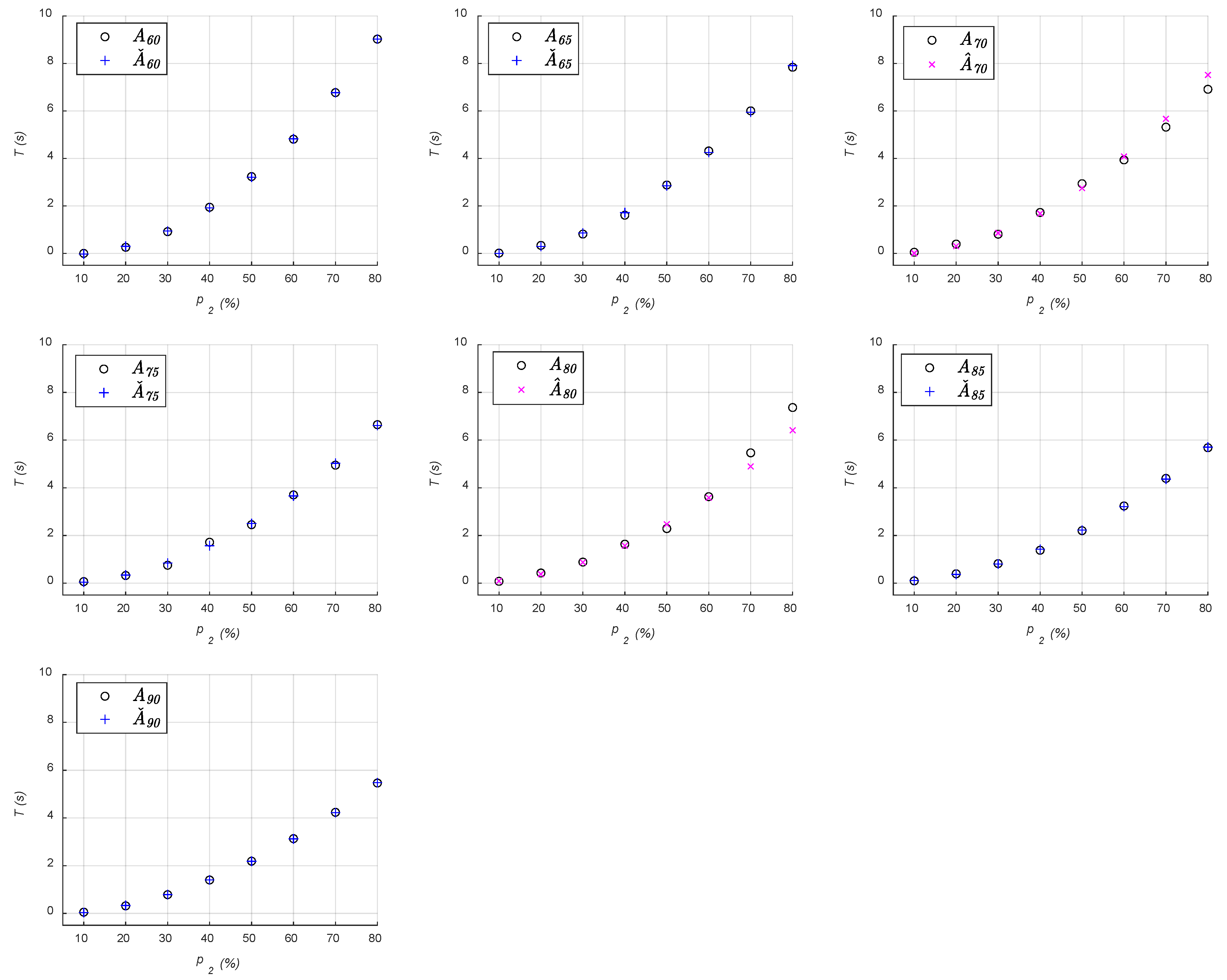
In
Figure 3, we observe that, for the
cases, the last two points of vectors
are clearly distant from the corresponding points of vectors
(in contrast with the other six points). The last two points are the
T when the percentage of slow vehicles is 70% and 80%. Hereafter,
is the mean error of the
x {1,2,…,5,6} procedure and the
y {1,2} comparison, where
y = 1 indicates a comparison between the directly modeled and observed data (
Table 26 or
Table 28), and
y = 2 indicates a comparison between the not directly modeled and observed data (
Table 27 or
Table 29). Then,
is the mean error of procedure 3 and
cases.
With procedure 1, the mean error between the directly modeled and observed data, i.e.,
, is lesser that the mean error between the not directly modeled and observed data, i.e.,
. This holds for the three procedures.
Figure 1 shows that, for
, the first six points of
and
are visible close to the corresponding points of
and
, respectively. The last two points of
are above those of
, and the last two points of
are below those of
.
In procedure 2,
varies between 0.2390 and 0.4151 s, and
is not distant from
s, so the error of the directly modeled data
is similar to the error of the not directly modeled data
.
Figure 2 shows that, for the directly modeled data (
), the first three points are above the observed data (
), point four is close (from above or below), points five to seven are below, and point eight is above. Comparing the indirectly modeled with the observed data, we notice that points 1, 2, and 3 of
are slightly above the corresponding points of
(for
cases
). For
, the estimated points 4 and 7 are visibly accurate, the estimated points 5 and 6 are below the observed value, and the estimated point 8 is above the observed value. For
, the estimated points 4 and 5 are visibly accurate, and the estimated points 6, 7, and 8 are below the observed value.
With these results, we found procedures 1 and 3 to be suitable to model the data for modeling and to explain the data for validating.
4.2. Discussion for Explaining V
Table 28 presents the error between the directly modeled data and data for modeling, with
.
Table 29 presents the error between the indirectly modeled data and data for validating, with
.
For modeling
V, procedure 6 is the best option. Here, we have that
and that
.
Figure 6 shows that, in vectors
for the
{60,65,75,90} cases, points 6 and 7 are the least accurate (i.e., dissimilar with the observed), with
being the most accurate (
= 0.0281 s) and
being the least accurate (
= 0.0956 s). In vector
, points 7 and 8 are the least accurate; therefore, when
= 80 km/h and for
= 70% and
= 80%, it was difficult to explain
V.In
Figure 5, and regarding the directly modeled data, points 5 and 6 of vectors
for the
cases are visibly inaccurate, and points 4 to 7 of vector
are also rather imprecise. Additionally,
has the highest error (
s) among
vectors of procedure 5, while
along with
present the lowest errors
. Regarding the indirectly modeled data, in vector
, points 5 to 7 are the least accurate, while in
, the least precise are points 5, 7, and 8. Hence, there are imprecisions when
and
for both of the
cases.
Procedure 4 presents the higher
, as can be seen in
Table 28 and
Table 29.
Table 28 shows that vectors
for the
cases {60,65,90} display
> 0.1.
Table 29 shows that vector
is more accurate than
, because
(0.1070 s < 0.1569 s).
With the results presented above, we consider procedures 5 and 6 as the best options for modeling and explaining the observed data. Besides, one important finding is that the pattern of V values, in the range to , is not the same among cases. It appears that a presence of about 50% of slow vehicles is the lowest threshold from where, and up to 80% in this study, the fast vehicles’ extra travel time variability follows a nonlinear pattern.
4.3. Contributions
The contributions of this study are as follows:
A better understanding of the traffic situations recreated through simulations, i.e., situations where vehicles traveling at different speeds interact with each other.
The developed procedures (and models within) for modeling and explaining the observed data from simulations. The best procedures in terms of a lower error were identified.
The patterns of T and V for each case and range were identified. T exhibited an identifiable pattern for all cases and ranges. For all cases and the range to 40%, V shows a linear pattern. For {60,65,75,80,90} cases and the range to 80%, V shows an unidentifiable pattern. For {70} case and the range to 80%, V shows an inverted U-shaped pattern. For case and the range to 80%, V shows a U-shaped pattern.
The findings of this work help to better understand heterogeneous traffic scenarios. The procedures can be used to describe the traffic of real locations and, with this information, authorities may decide which actions are required to alleviate traffic issues. Moreover, the traffic outcome of possible future scenarios can help to better plan public infrastructure that avoids congestions, low speeds, high noise levels, pollutions, and other problems that arise as a result of traffic problems.
4.4. Practical Application
A two-lane, one-direction avenue is a common infrastructure in street networks of heterogeneous traffic, i.e., where different types of vehicles circulate and where the vehicles’ desired speed may not be the same. Examples of this infrastructure are the avenues’ segments described in
Table 30.
The two segments described in
Table 30 are separated by a sidewalk and the posted speed limit for both is 60 km/h, despite that it is common that vehicles traveling at a lower speed than the speed limit slow down the traffic. The procedures introduced in the present study were developed with the intention of analyzing the traffic of segments with similar features to those presented in
Table 30. After calibration, the models describe the average extra travel time and the extra travel time variability of the fast vehicles according to the percentage of slow vehicles circulating and the desired speeds. With this information, the corresponding authorities can adjust (or create) policies for restricting or penalizing the slow vehicles in order to keep a desired level of service, or to simply inform users of the current level of service.
5. Conclusions
Procedures 1, 2, and 3 model and explain the mean extra travel time (dependent variable) through the percentage of slow vehicles (independent variable). Procedures 1 and 3 accurately modeled the data for modeling, with procedure 2 being the least accurate. Moreover, procedures 1 and 3 are accurate for explaining the data for validating, both for to 60%, but less accurate for and 80%, concluding that, when the percentage of slow vehicles is 70% or more, it became difficult to explain the data for validating.
Procedures 4, 5, and 6 model and explain the extra travel time variability (dependent variable). In procedure 4, the independent variable is the mean extra travel time, and in procedures 5 and 6, it is the percentage of slow vehicles. Procedure 4 is the least accurate to model the data for modeling and to explain the data for validating, therefore is a better choice of independent variable than T. Procedures 5 and 6 modeled the data for modeling at approximately equal accuracy. Procedure 5 presents the higher error for , being least precise in the range to 70%. Procedure 6 presents the higher error for , being least precise at and 70%. Moreover, procedures 5 and 6 explain with approximately the same accuracy the data for validating. For procedures 5 and 6, we can say that, in and , in the range to 40%, the V values (the corresponding observed values present a linear pattern) in general are better explained than in the range to 80%, although in the last range with , the observed V values likely present an inverted U-shaped form, and with , a U-shaped form.


