Bionic Artificial Lateral Line Underwater Localization Based on the Neural Network Method

Abstract

The lateral line system is an essential mechanosensory organ for organisms such as fish; it perceives the fluid environment in the near-field through the neuromasts on the lateral line system, supporting behaviors (e.g., obstacle avoidance and predation in fish). Inspired by the near-field perception ability of fish, we propose an artificial lateral line system composed of pressure sensors that respond to a target’s relative position by measuring the pressure change of the target vibration near the lateral line. Based on the shortcomings of the idealized constrained modeling approach, a multilayer perceptron network was built in this paper to process the pressure signal and predict the coordinates on a two-dimensional plane. Previous studies primarily focused on the localization of a single dipole source and rarely considered the localization of multiple vibration sources. In this paper, we explore the localization of numerous dipole sources of the same and different frequency vibrations based on the prediction of the two-dimensional coordinates of double dipoles. The experimental results show that the mutual interference of two vibration sources causes an increase in the localization error. Compared with multiple sources of vibration at the same frequency, the positioning accuracies of various vibration sources at different frequencies are higher. In addition, we explored the effects of the number of sensors on the localization results.

1. Introduction

With the continuous development of human scientific and technological civilization, the resources and spaces in the ocean have become more important as a proportion of national resource development. The development of marine resources and the protection of maritime rights and interests are integral parts of achieving a solid ocean state, which is of great strategic importance for all countries [1,2]. At the same time, to build a power ocean, it is imperative to develop appropriate underwater detection equipment and related technologies; underwater positioning technology is the most critical underwater detection technology, and how to perform accurate positioning in the complex ocean environment is a problem that needs to be urgently solved.

In traditional underwater detection technology, acoustic-based underwater localization techniques have been widely studied by researchers [3,4,5]. They have achieved good localization results, but near-field targets are susceptible to mutual interference, such as noise between marks [6,7]. Sonar and visual detection technology in a specific environment (narrow space, turbid waters) is ineffective. Due to the natural shielding effects of seawater, the GPS positioning of land navigation cannot be used for underwater positioning. The complex environment, such as ocean noise, interferes significantly with the perceived effect of sonar, and the traditional optical detection equipment is limited by underwater refraction, insufficient light, and other factors [8,9]. To solve these problems, the underwater detection equipment can sense the target position in the near-field environment and guarantee the successful execution of the mission of underwater detectors. The development of a new underwater positioning technology is an urgent need.

Fish and some amphibians have susceptible underwater perceptions of the lateral line system on both sides of the fish body. The lateral line system is an essential organ for fish and these amphibians to obtain information about their surroundings [10,11]. With the help of this organ, fish and these amphibians can perform behaviors, such as clustering, prey localization, obstacle avoidance, and target recognition in complex underwater environments. The aquatic environment is complex and variable. When light conditions in the external environment are insufficient, fish rely on their unique lateral line perception systems to sense information about the surrounding flow field [12,13,14]. A more representative one is the Mexican cavefish, which has lived in this way under dark conditions for a long time [15].

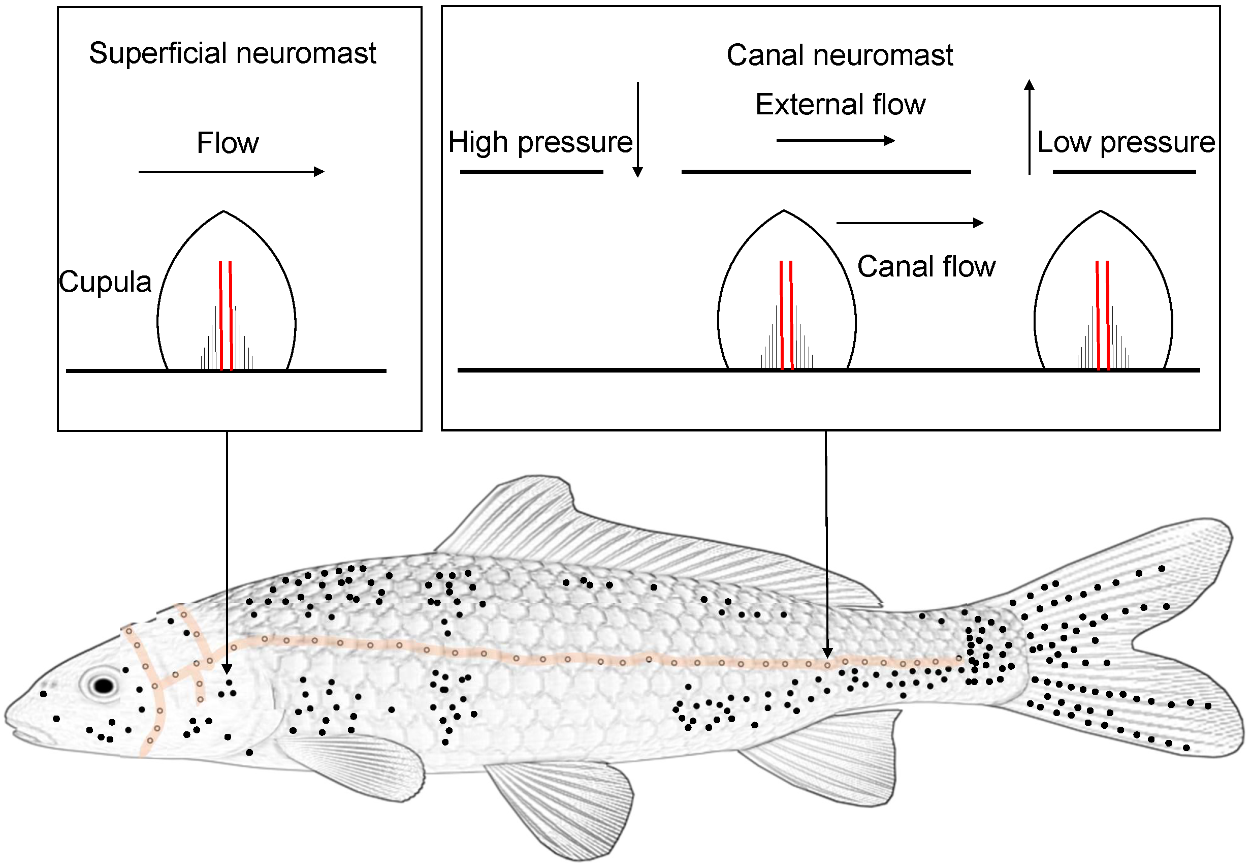
The lateral line system of fish consists of two main components: the superficial neuromast, which perceives the flow velocity in the near-field environment, and the canal neuromast, which is sensitive to pressure changes in the near-field environment [16], as shown in Figure 1. The perceptual functions of these two structures differ because of their different distributions on the lateral line system and differences in their structuring [17,18]. It has been shown that the superficial neuromast is more sensitive to velocity changes in the flow field. In contrast, the canal neuromast can respond better to pressure changes in the flow field environment [19]. Based on the properties and mechanisms of the fish lateral line system to perceive the surrounding flow field, it provides a new idea for the underwater localization of the underwater detector to accurately perceive the surrounding near-field environment.

In this paper, we propose using an array of integrated pressure sensors to locate dipole sources in the near-field. Similar to the lateral fish line, the sensor arrays are arranged in parallel and are more compact compared to the cross-type arrangement. In addition, based on the collected pressure variation data, we constructed a multilayer perceptron (MLP) neural network algorithm for dipole source localization. With the flexibility of the network structure, strong nonlinear capability, and strong robustness, the multi-layer perceptron network (MLP) is outstanding in solving nonlinear problems. It has been widely used in control systems, biomedicine, agriculture, data management, environmental engineering, and other fields [20,21,22,23,24]. Considering the small number of samples collected in the experimental environment, we used data augmentation to expand the number of samples. For example, the original data samples were equally segmented, and fast Fourier transform extracts the sub-samples. For the frequency multiplication phenomenon that occurs in the signal, we attempted to extract the frequency multiplication signal as a feature and found that this move could significantly improve localization accuracy.

Most of the existing studies focus on the localization of single dipole sources and rarely consider the localization of double dipole sources. This is because the flow field formed by a double dipole source is more complex than that of a single dipole source, and interference and superposition may occur between the waves generated by the two spheres. Based on the data augmentation of single dipole source localization and the method of extracting multiplier signals as features, we explored the problem of localization of double dipole sources at the same and different frequencies. The experimental results show that the localization of double dipole sources at different frequencies is more accurate than localization at the same frequency. This is mainly because the features extracted from the data collected at different frequencies are more significant.

The main contributions of this work are as follows:

1.

In this paper, we used the MLP network. Based on the time domain signal of the pressure variation obtained from the experimental acquisition, we used the time-frequency analysis method to extract the frequency domain features as the input to the network. By analyzing the frequency domain of the call, we found that the sign appears to be a frequency doubling phenomenon, so we investigated the feasibility of the frequency-doubled movement as the effective signal. The experimental results show that the increase of the feature dimension improved the accuracy of localization.

2.

In this paper, we explored the little-studied dual-vibration source localization. We investigated the effects of the differences in frequencies on the localization results from the perspective of the same and different frequencies, respectively. The experimental results show that, compared to single dipole localization, the error of double dipole localization increases for the same frequency, and the error of double dipole localization for different frequency vibrations shows a decreasing trend.

3.

In this paper, we investigated the influence of the arrangement and number of sensors on localization, and how to obtain the best localization effects by reasonable and adequate performances with a certain number of sensors. The experimental results show that increasing the number of sensors and space dimensions can improve the localization accuracy to a certain extent.

The remainder of the paper is organized as follows. The related works about the design of the artificial lateral line array and algorithm of underwater localization are presented in Section 2. The perception method and experiment set are presented in Section 3 and Section 4, respectively. Experimental results on localization—both the single dipole source and double dipole source—are discussed in Section 5. Finally, the conclusion is provided in Section 6.

2. Related Work

For the underwater target localization problem, most of the related works focus on the dipole source localization perspective, because the flow field changes generated by the fins and tails of underwater animals are similar to the flow field formed by the dipole source. The localization for underwater targets can be simplified to dipole localization [25]. In previous studies, many kinds of artificial lateral arrays have been designed and fabricated for the localization and tracking of underwater targets. The flow field information was obtained by these artificial arrays and information processing methods to predict the position or the direction of motion of the target, and some breakthrough results were obtained. The following summarizes the previous work from two aspects: array design and information processing methods of neural networks.

2.1. Design of Artificial Lateral Line Array

Artificial cilia sensor arrays designed by simulating the structure of the superficial neuromast (SN) are more representative designs [26,27,28,29,30,31,32]. For example, Liu et al. developed a cross-cross-shaped artificial lateral array by designing a sensor that mimics a cilia bundle to successfully localize a dipole source, verifying the sensing capability of artificial laterals [28,29]. Asadnia et al. created a novel sensor by mounting polymer cilia with electrodes at the bottom, fabricated by stereolithography, on a thin film, and a one-dimensional array of 10 such sensors. A one-dimensional array composed of such sensors responded well to dipole stimulation [32].

Another part of the lateral line system is the canal neuromast (CN), which is a primary morphology (one of them) of the fish lateral line system and is the most visual representation of the lateral line system of the fish trunk [33]. The design and fabrication of bionic sensors that mimic the CNs are also hot spots explored by related scholars [34,35,36,37,38]. For example, Jiang et al. developed an artificial pipeline array by integrating a cantilevered sensing unit in polydimethylsiloxane (PDMS) with a high-pass filtering capability to attenuate low-frequency stimuli [34]. Liu et al. developed an artificial lateral array, mimicking pipeline laterals by encapsulating an artificial cilia sensor inside an open-hole pipeline and simulating the structure of a lateral pipeline neural mound; compared to the sensor, directly exposed to the fluid, the construction of the mimic pipeline lateral line can effectively suppress the noise [38].

Artificial sideline arrays developed using commercial pressure sensors for dipole source detection have also received extensive attention and intensive research [39,40,41]. For example, Jiang et al. developed a sideline array integrating IPMC velocity modal and pressure sensors to achieve multimodal sensing fusion and reduce localization errors [39].

In summary, researchers have conducted much work in simulating lateral line systems for structural mimicry and the rapid development of lateral line arrays using commercial sensors. Various sensors and artificial lateral line arrays have been designed and developed based on different sensing principles, which are becoming closer to biological lateral line systems in structure, and their performances are gradually improving. However, there is still a significant gap in the sensing capability of the existing physical lateral line system. Most of the research focuses on the lateral line arrays themselves, and the actual sensing capability of the lateral line arrays needs to be further investigated.

2.2. Neural Network Approach for Underwater Localization

Various signal processing methods have been used for signal processing for underwater localization. It is divided into two main directions. First, building a dipole source flow field model and using different constraint methods to resolve the model [7,42,43,44]. Second, a neural network modeling method was built to mimic the fish in a complex environment by training over a long period to complete various activities and behaviors, building neural networks to process the received signals. Abdulsadda et al. used a multilayer perceptron network (MLP) to extract pressure amplitudes as features for localization [26]. Zheng et al. used generalized regression networks for underwater localization experiments [41]. Liu et al. used artificial neural networks (ANNs) to identify the coordinates, frequency, and amplitude of vibration sources and achieved an accuracy of 93% [45]. Jiang et al. achieved dipole source localization in 2D and 3D using MLP networks [39]. Wolf et al. used the long short-term memory (LSTM) model to process pressure-varying time series data. They were able to effectively improve the robustness of the network using the memory function of the LSTM model [46].

Previous research has shown that using artificial neural networks for underwater localization is an effective method. However, collecting data based on experimental platforms causes insufficient data volume, which makes the neural network lack sufficient training and causes overfitting. In addition, most of the studies focus on the localization of a single dipole source; in fact, most situations underwater have multiple objects moving at the same time, and the research on how to perform accurate localization under the conditions of interference from various things needs to be further studied.

3. Method

The characteristic parameter estimation algorithm (based on the target flow field model and some ideal condition assumption constraints) is very different from the actual flow field environment, making the localization in practical experiments ineffective. This paper proposes a neural network-based underwater target localization method that discards the need for accurate modeling and trains a neural network model using pressure data collected by an artificial lateral line sensor array for underwater target localization.

3.1. All Principles of Perception

The artificial lateral line array passes through the fluid medium and measures information about the pressure variation of the vibrating source to describe the flow field variation of the target, which can be explained by the theory of potential flow [47]. The flow field variation generated by an underwater target can be reduced to a dipole source model. A typical dipole source is generated by a constant frequency sinusoidal vibration of a rigid sphere of continuous volume [48].

As shown in Figure 2, the target sphere $\left(x_s,y_s\right)$ moves up and down sinusoidally perpendicular to this plane with amplitude A and displacement equation $S=Asin\omega t$. At the sensor $\left(x_1,y_1\right)$, the pressure change $p\left(i\right)$ that can be received is [45]:

$$p\left(i\right)=\rho \frac{R^{3}S{\omega }^2}{2}·\frac{x_s-x_1}{{\left({\left(x_s-x_1\right)}^2+{\left(y_s-y_1\right)}^2\right)}^{\frac{3}{2}}}$$

(1)

3.2. Neural Network Algorithm for Localization

The pressure variation information collected from the artificial lateral line array sensors is complex (concerning the vibration source). It can lead to significant deviations from the ideal pressure signal in practical measurements. For example, the boundary conditions of the tank tend to produce factors such as the motion between waves, non-ideal fluids, and sensor arrays. The variability between sensors due to manufacturing factors and the zero point drift that occurs during sensor use can lead to interference with the analog signal output from the detector [49]. Therefore, it is not easy to obtain the ideal analytical solution by building an accurate flow field model to calculate the coordinates of the vibration source. Fish extract helpful information from the surrounding noise-filled flow field environment based on their well-developed biological neural networks. Inspired by this physiological mechanism, we used neural networks to process pressure signals.

MLP is a very typical feedforward neural network consisting of an input layer, multiple hidden layers, and an output layer, and it is the most widely used network structure for nonlinear prediction and classification [50]. Moreover, due to the simple design, adaptive learning capability, and robust noise performance [51], MLP networks are used in many research works to process signals on sideline sensors. The MLP network used in this paper is shown in Figure 3; its input dimension was the number of manually extracted features. We chose to use frequency domain features as the input features of the network. The time domain signal was first processed using FFT, and then the amplitude at the blob vibration frequency or the corresponding octave frequency was extracted as the input to the network.

4. Experiment Setup

In this section, we describe the construction of the experimental setup, the design of the sensing array, the calibration of the sensors, the preprocessing of the data, and the setting of the hyperparameters of the network.

4.1. Experiment Device

All experimental results were performed on a platform built in the laboratory. The testing platform mainly contained a 100 × 50 × 50 cm water tank filled with silicone oil at a depth of 15 cm, as shown in Figure 4. The artificial lateral line array was fixed at the center of the water tank by an aluminum rod set at the center of the platform and moved to 8 cm underwater (the upper surface from the horizontal) for positioning the experiment. A 50 mm diameter ball was attached to the shaker by a stainless iron rod of 200 mm in length and 5 mm in diameter, and the ball vibrated vertically along the height direction of the water tank. The drive of the ball to produce sinusoidal motion was generated by a signal generator and amplified by a power amplifier, which transmitted the sinusoidal signal to the shaker, making the shaker drive the ball to produce sinusoidal motion. The frequency and amplitude of the sinusoidal motion of the ball can be adjusted by the signal generator and the power amplifier.

The vibrator was mounted on a filament holder that allowed the position of the slight ball vibration to be adjusted by a stepper motor. The fixing frame of the lateral line array was not in contact with the tank and the fillet holder to avoid the noise caused by the vibration from interfering with the pressure variation data. Section 2 mentions that the frequency of the fish lateral line pipeline neural mound response is between a few Hz to tens of Hz, so this paper selected a frequency of 8 Hz for single vibration source positioning experiments and used 10 Hz and 8 Hz for double vibration source positioning experiments at different frequencies, which was within the response range of the lateral line system. A vibration direction is a vertical-horizontal plane and the amplitude of vibration at 8 Hz frequency is about 3.2 mm, and the vibration amplitude at 10 Hz frequency is about 3.7 mm.

4.2. Design of Sensor Array and Sensor Calibration

The artificial lateral line sensor we designed mainly mimicked the function of the ductal neural mound of the lateral line system of the fish trunk, and the system as a whole resembled the shape of the fish trunk. The design took two parallel rows, as shown in Figure 5c, and each row consisted of four Freescale pressure sensors MPXV5004GC6U powered by a 5 V power supply, as shown in Figure 5d. The sensors were distributed at equal intervals of 25 mm along the horizontal direction with a distance of 30 mm between two rows, as shown in Figure 5a,b. The purpose of this design was to capture more pressure variations in the flow field and to facilitate the localization of the dipole source. The body length was defined as the maximum length of the sensing array, and on the system we designed, the maximum length (body length) was 100 mm.

Although the sensors were factory calibrated for sensitivity, there was a reasonable error in the sensitivity of the sensors due to the factory process. To ensure the correctness of the pressure signal for dipole positioning, we calibrated this batch of sensors using a digital pressure sensor. The signal amplitudes of the sensors used for the experiments in the laboratory environment are shown in Figure 6, and

Table 1. Sensitivity of 8 sensors after calibration.

Pressure Number	Proportional Constant (Mpa/V)	Pressure Number	Proportional Constant (Mpa/V)
${\mathbf{P}}_1$	0.103	${\mathbf{P}}_5$	0.079
${\mathbf{P}}_2$	0.081	${\mathbf{P}}_6$	0.078
${\mathbf{P}}_3$	0.082	${\mathbf{P}}_7$	0.092
${\mathbf{P}}_4$	0.084	${\mathbf{P}}_8$	0.101

shows the sensitivity of each pressure sensor after calibration.

4.3. Data Pre-Processing

We conducted experiments on the localization of single and double dipole source vibrations in the two-dimensional plane. To determine the relative positions of the dipole spheres, we set the coordinate system at the location of the central axis of the sensor array as the coordinate origin. To train the neural network model, the plane 140 × 240 mm was divided into a 20 × 20 mm grid to form 91 data acquisition points. Five sets of data were acquired at each acquisition point for 455 collections of experimental data. The data sampling frequency was 1000 Hz, and 14 seconds of data were collected each time, totaling 14,000 data points. These data were randomly divided into a training set and a test set according to a ratio of 8:2. The ball was moved at each data collection point, and the obtained pressure signal was used to train the neural network.

Figure 7 shows the pressure vibration signal acquired by the pressure sensor when the sphere was at the (20 mm, 0 mm) position. Using MATLAB’s time-frequency tool, the time domain signal acquired by the pressure transducer could be converted into the frequency domain signal by using the fast Fourier transform (FFT).

For the MLP network, we converted the signal into a frequency domain signal, extracted the output voltage amplitude at a specific frequency, multiplied it by the individual pressure sensor sensitivity to obtain the pressure amplitude, and then normalized the data.

$$S_j^{\prime }\left(i\right)=\frac{S_j\left(i\right)-S_j\left(M\right)}{S_j\left(\sigma \right)}$$

(2)

here, $S_j\left(i\right)$ denotes the signal amplitude of sensor j. $S_j\left(M\right)$ and $S_j\left(\sigma \right)$ are the mean and standard deviations of sensor j, respectively.

4.4. Data Augmentation

Considering that the amount of data in the training set is too small, we chose to cut each copy of 14,000 data points equally for the data augmentation processing. At the same time, we could explore the influence of different data-cutting methods on the training results. From the frequency domain signal of the original data, there was a multiplication phenomenon in the pressure data, which may have been due to the limitations of the boundary conditions of the experimental platform leading to the interference superposition between the waves generated by the vibration, etc. Since all the data were collected at the same venue, the multiplication signals could be considered valid signals to a certain extent.

Generally, the pressure amplitude of the minor ball vibration frequency was selected as the input feature of the MLP network because the multiplier signal was prominent; we also likened the multiplier amplitude to the feature and compared the results with and without the multiplier signal. The data could be equally divided into 2 or 14 parts and combined with the extracted features method. The method of combining the single sphere vibration data of MLP-1 to MLP-6 is detailed in

Table 2. Classification of several data augmentation and feature extraction methods.

Method	Data Segmentation	Feature Amplitude
MLP-1	(14,000, 1)	8 Hz
MLP-2	(14,000, 1)	8 Hz, 16 Hz, 24 Hz, 32 Hz
MLP-3	(7000, 2)	8 Hz
MLP-4	(7000, 2)	8 Hz, 16 Hz, 24 Hz, 32 Hz
MLP-5	(1000, 14)	8 Hz
MLP-6	(1000, 14)	8 Hz, 16 Hz, 24 Hz, 32 Hz
MLP-7	(14,000, 1)	8 Hz
MLP-8	(14,000, 1)	8 Hz, 16 Hz, 24 Hz, 32 Hz
MLP-9	(7000, 2)	8 Hz
MLP-10	(7000, 2)	8 Hz, 16 Hz, 24 Hz, 32 Hz
MLP-11	(1000, 14)	8 Hz
MLP-12	(1000, 14)	8 Hz, 16 Hz, 24 Hz, 32 Hz
MLP-13	(14,000, 1)	8 Hz, 10 Hz
MLP-14	(14,000, 1)	8 Hz, 16 Hz, 24 Hz, 32 Hz 10 Hz, 20 Hz, 30 Hz, 40 Hz
MLP-15	(7000, 2)	8 Hz, 10 Hz
MLP-16	(7000, 2)	8 Hz, 16 Hz, 24 Hz, 32 Hz 10 Hz, 20 Hz, 30 Hz, 40 Hz
MLP-17	(1000, 14)	8 Hz, 10 Hz
MLP-18	(1000, 14)	8 Hz, 16 Hz, 24 Hz, 32 Hz 10 Hz, 20 Hz, 30 Hz, 40 Hz

. The data segmentation part of the table indicates the features of the sample data, for example, (7000, 2), where 7000 indicates the length of this training batch sample data and 2 shows the number of equal parts of the original data. The amount of the feature amplitude means the amplitude on a specific frequency is extracted.

For the double dipole localization experiments, we explored the effects of the same-frequency and different-frequency vibrations on the localization results. For the same-frequency vibration, we extracted the amplitude of 8 Hz and its multiples as the feature input. For the different-frequency vibration, we extracted the amplitudes on 8 Hz and 10 Hz, and their multiples as the feature inputs, respectively. The combination with the data increment method is detailed in Table 2 for MLP-7 to MLP-18.

MLP-7 to MLP-12 are experimental combinations of double dipole localization with same-frequency vibrations and MLP-13 to MLP-18 are experimental combinations of double dipole localization with different-frequency vibrations. To ensure the comparability of the experimental results, the hyperparameters of the MLP network used for a single dipole localization and double dipole localization were kept the same.

4.5. Hyperparameter Setup

The setting of hyperparameters is self-explanatory for how well the network model fits. First, the number of input nodes in the MLP network is equal to the feature input dimension. For example, when using the model to train single dipole localization experimental data, the number of input nodes should be set to 8 if only the amplitude at the vibration frequency is extracted as a feature and 32 if the amplitude at the multiplier frequency is added as a feature. Second, each output node represents the predicted coordinates of each dipole on each axis. Each hidden layer node represents a nonlinear activation, which takes the ReLU function as the activation function.

$$f\left(x\right)=max(0,x)$$

(3)

The training set for the localization experiments consists of a series of known dipole coordinates and the corresponding pressure amplitudes from the sensor signals. Parameters, such as the number of hidden layers and nodes and the learning rate, are determined by the optimal network structure obtained through training.

We first conducted a single dipole localization experiment on a plane with 91 positions. There were 72 training points and 19 test points according to the ratio of 8:2. The optimal network structure was determined after constant tuning of the experiments on single dipoles. The optimal network structure had two hidden layers, and the numbers of nodes in the hidden layer were 100 and 50, respectively. The number of epochs was set to 1000, and the learning rate was set to 0.001. To achieve better comparability of the results, the hyperparameters of the experimental training network for double dipole localization were kept the same as those of the single dipole training network.

5. Result and Discussion

This section presents the localization results of dipoles. The localization accuracy was improved as more feature dimensions were extracted from the signal. This advantage can be visualized in the localization results for single- and multi-source vibrations. The localization results for multi-source vibrations with different frequencies were more prominent than those with the same frequencies. Finally, we investigated how the arrangement and number of sensors affected localization accuracy.

5.1. Experimental Localization Results for a Single Vibration Source

Figure 8 shows the localization results of the single dipole in the two-dimensional plane. The blue square dots and red dots indicate the actual and predicted positions of the test points, respectively, and the rest are the training data points. To characterize the test results, we used the absolute errors of the positions in the x and y directions of the training set and the average Euclidean distance error to judge the training results, respectively. The following equation defines the Euclidean distance error.

$$ED=\sqrt{{\left(x_i-X_i\right)}^2+{\left(y_i-Y_i\right)}^2}$$

(4)

$x_i$ and $y_i$ represent the predicted x and y coordinates, respectively. $X_i$, $Y_i$ denote the actual x and y coordinates, respectively.

Figure 8a–f show the results of different data segmentation and feature extraction methods for individual dipole localization, respectively. As shown in

Table 3. The mean absolute error of the results in FIG-8.

Method	MAE-x (cm)	MAE-y (cm)	MED (cm)
MLP-1	0.6711	0.8391	1.1547
MLP-2	0.3318	0.4359	0.5868
MLP-3	0.9552	0.9710	1.4678
MLP-4	0.3093	0.4252	0.5691
MLP-5	0.6199	0.6886	1.0348
MLP-6	0.5269	0.7028	0.9334

, when the data are divided equally into two, and only the amplitude at 8 Hz is extracted as the feature, the mean Euclidean distance (MED), mean absolute error along the x-axis (MAE-x), and mean absolute error along the y-axis (MAE-y) are 1.4678, 0.9710, and 0.9552 cm, respectively, while the data are divided equally into two. The amplitudes at the vibration frequency and octave are extracted as the features; the MED, MAE-x, and MAE-y are reduced to 1.4678, 0.9710, and 0.9552 cm, respectively. In addition, similar results can be obtained to compare MLP-2 and MLP-1, MLP-6, and MLP-5. Based on the localization results of the single two-dimensional dipole, we can conclude that the localization accuracy can be significantly improved by upgrading the feature dimension.

Figure 9 shows the absolute error between the actual and predicted positions of the 19 test points of MLP-3 and MLP-4.

5.2. Experimental Localization Results for the Double Vibration Source

We conducted multi-source vibration experiments at the same frequency and at different frequencies to investigate the effect of the difference in frequency on the two-dimensional positioning of the multi-source dipole. In contrast to the grid points regularly divided by a single dipole source, we randomly generated 100 sets of two spheres to vary the relative positions of two dipoles. We set the dipole coordinates closer to the lateral line system as $\left(x_1,y_1\right)$ and the coordinates of the more distant dipole as $\left(x_2,y_2\right)$. Where, considering the hardware conditions, the two dipole coordinates satisfy: $x_1\in \left[2,4\right]$, $x_2\in \left[12,14\right]$, $\left|x_1-x_2\right|\ge 10$, $y_1,y_2\in \left[-8,8\right]$.

In the following, we will explore the effects of the vibrations of the same and different frequencies on the localization of the double dipole from the differences and similarities of the vibrations.

5.2.1. Same Frequency Multi-Source Vibration Localization Results

Figure 10a–f shows the multi-source dipole two-dimensional localization results by different data segmentation and feature extraction methods, respectively. From the localization error statistics in

Table 4. The mean absolute error of the results in FIG-10.

Method	MAE-x${}_1$(cm)	MAE-y${}_1$(cm)	MED${}_1$(cm)	MAE-x${}_2$ (cm)	MAE-y${}_2$ (cm)	MAD${}_2$(cm)
MLP-7	0.3378	0.4813	0.6153	0.6119	2.1918	2.3547
MLP-8	0.1727	0.2428	0.3147	0.3877	0.8551	1.0042
MLP-9	0.1475	0.2565	0.3162	0.4415	2.3220	2.4308
MLP-10	0.1303	0.1391	0.2188	0.3786	0.7005	0.8741
MLP-11	0.1160	0.1156	0.1749	0.4525	2.7091	2.8520
MLP-12	0.1155	0.1151	0.1784	0.2853	1.4828	1.5730

, the localization error of the spheres closer to the artificial lateral line (ALL) is much smaller than the localization error of the spheres farther away from the ALL, regardless of the combination method. Comparing MLP-7, MLP-9, and MLP-11, the MED of the closer spheres decreases from 0.6153 to 0.3162 cm and then decreases to 0.1749 cm as the segmentation increases (i.e., the amount of data becomes more extensive). This result indicates that the neural network fits better as the data increase. Similar results are obtained when comparing MLP-8, MLP-10, and MLP-12.

Although increasing the dimensionality of the feature by extracting the amplitude of the multiplier can reduce the error, for example, from the localization results of MLP-9 and MLP-10, the MED of the more distant sphere plummets from 2.4308 to 0.8741 cm. However, the localization error of the more distant globe from the ALL is generally significant, indicating that the network does not accurately localize the more distant sphere. This is mainly because both dipoles vibrate at 8 Hz, making the signal from the more distant blob quickly drowned out by the call from the closer chunk. The MLP network input is the amplitude feature, which makes the features of the more distant sphere not effectively represented.

5.2.2. Different Frequency Multi-Source Vibration Localization Results

Figure 11a–f shows the experimental localization results of different data segmentation and feature extraction methods. From the localization error statistics in

Table 5. The mean absolute error of the results in FIG-11.

Method	MAE-x${}_1$(cm)	MAE-y${}_1$(cm)	MED${}_1$(cm)	MAE-x${}_2$(cm)	MAE-y${}_2$(cm)	MAD${}_2$(cm)
MLP-13	0.1933	0.2094	0.3037	0.2709	0.4643	0.5688
MLP-14	0.0718	0.0734	0.1157	0.2094	0.3573	0.4382
MLP-15	0.0907	0.1834	0.2160	0.3752	0.6794	0.8296
MLP-16	0.1187	0.0839	0.1577	0.1866	0.3052	0.3970
MLP-17	0.0751	0.0675	0.1117	0.2565	1.1492	1.2086
MLP-18	0.0820	0.1009	0.1469	0.1444	0.8245	0.8563

, because the two spheres vibrate at different frequencies, even the spheres far from the ALL are accurately localized. From the localization results of MLP-13, even if only the amplitudes of 8 and 10 Hz were extracted, the MED errors of the pellets closer to the ALL and the bullets further away from the ALL were 0.3037 and 0.5688 cm, respectively, which were at a relatively low level. As the number of data increases, for example, comparing the localization results of MLP-13, MLP-15, and MLP-17 for the closer blob, the localization error of the more relative chunk has a decreasing trend. Its MED, MAE-x, and MAE-y decreased from 0.3037 cm, 0.1933 cm, and 0.2094 cm to 0.1117 cm, 0.0751 cm and 0.0675 cm; however, this trend was not reflected in the more distant blob.

The results of both MLP-14 and MLP-16 are better, and their MED errors on the two blobs are about 0.1 cm and 0.4 cm. MLP-14 and MLP-16 extract the amplitudes on 8 Hz and 10 Hz and their multiples for eight feature dimensions. This result indicates that increasing the dimensionality of the features improves the fitting ability of the network.

5.3. Effect of Sensor Arrangement and Number on Localization Error

How to obtain better positioning results by a reasonable arrangement with a certain number of sensors was the focus of this paper. In this paper, two parallel rows of sensor arrays were divided into three contracts for comparison with the use of sensors; the sensors were numbered S1, S2, S3, and S4 from left to right from the first row, and similarly, the second row was divided into S5, S6, S7, and S8 respectively. We have divided four permutations, as detailed in

Table 6. Classification of different combinations of sensors.

Type	Sensor Number	Number of Sensor
Type-1	S1, S2, S3, S4	4
Type-2	S5, S6, S7, S8	4
Type-3	S2, S3, S6, S7	4
Type-4	S1, S2, S3, S4, S5, S6, S7, S8	8

.

The localization experiments for single and multiple vibration sources were performed using different distributions and numbers of sensors. To better represent the localization results, we used the best combination of data segmentation and feature extraction methods, respectively. For the single-source vibration, we used a combination method similar to MLP-4, and for a multi-source beat, we used MLP-10 and MLP-16, respectively.

Figure 12 and

Table 7. The mean absolute error of the four arrangements.

Method	MAE-x (cm)	MAE-y (cm)	MED (cm)
Type-1	0.4813	0.6233	0.8447
Type-2	0.4675	0.6359	0.8356
Type-3	0.5187	0.6625	0.8937
Type-4	0.3093	0.4252	0.5691

shows the results of the sensor arrangement and number for localization of a single dipole. Type-1 and Type-2 have close errors in MAE-x, MAE-y, and MED, with values around 0.5, 0.6, and 0.8 cm. Type-3 has higher errors than both Type-1 and Type-2 because Type-3 has two sensors per row in the vertical direction. Although the total number of sensors is the same as Type-1 and Type-2, a lot of 2D spatial information is missing when performing 2D dimensional localization. In addition, the localization error decreases significantly when a whole part of the sensor is used. This result guides the design of 2D arrays of sensors and the number of sensors can be increased on a 1D display to improve the accuracy of the sensors.

Figure 13 shows the results of the localizations of multi-source vibrations for different sensor arrangements and numbers. Figure 13a shows the results for the same frequency vibration and Figure 13b shows the results for different frequencies. Among them, the errors of the localization results for Type-1 and Type-2 are similar in absolute error for both dipoles, indicating that the one-dimensional lateral line array can be performed regardless of the single dipole localization or multiple dipole localizations.

The localization error is more significant for the dipole further away from the ALL for multiple dipole localizations. When vibrating at the same frequency, the MAE-x and MAE-y of Type-3 increased by 44.9% and 78.4% year-on-year relative to Type-2. The MAE-x and MAE-y increased by 27.2% and 32.1% year-on-year for Type-3 close to Type-2 when vibrating at different frequencies. The results show that the number of sensors on the 1D array was the key to the 2D localization accuracy.

6. Conclusions

This paper presents the ALL system with an integrated pressure sensor and the method of underwater localization using an MLP neural network. To compensate for the lack of data, a data augmentation method was used to segment the collected data, increasing the amount of data for the experiment and reducing the localization error. Due to the limitation of the experimental boundary, the signals were inevitably multiplied, and there was a connection between the multipliers of the signals due to the uniqueness of the testing platform. The localization results based on a single dipole proved that the signal’s multiplier signal was not noise. The localization results were better when the multiplier signal was used as a valid signal than when the amplitude of the vibration frequency was extracted singly. Based on the results of multiple dipole localization, the vibrations of different frequencies increase the dimensionalities of the extracted features and dramatically reduces the localization errors of two dipoles.

The experimental results of the multi-source vibration localization at different frequencies show that the MLP network can predict dipole coordinates well, as long as the features are suitable and the dimensionality is sufficient. However, the drawback of this method is that it requires artificially provided features, and it cannot achieve accurate localization when it encounters the same frequency vibration and cannot extract more features. Based on this, in future work, convolutional neural networks can be used to exploit the data information fully. In addition, the development of smaller and high-precision sensors and the realization of data fusion between different sensors are also bases for achieving the precise positioning of underwater targets.