
Self-Anti-Disturbance Control of a Hydraulic System Subjected to Variable Static Loads


Abstract
:Featured Application
Abstract
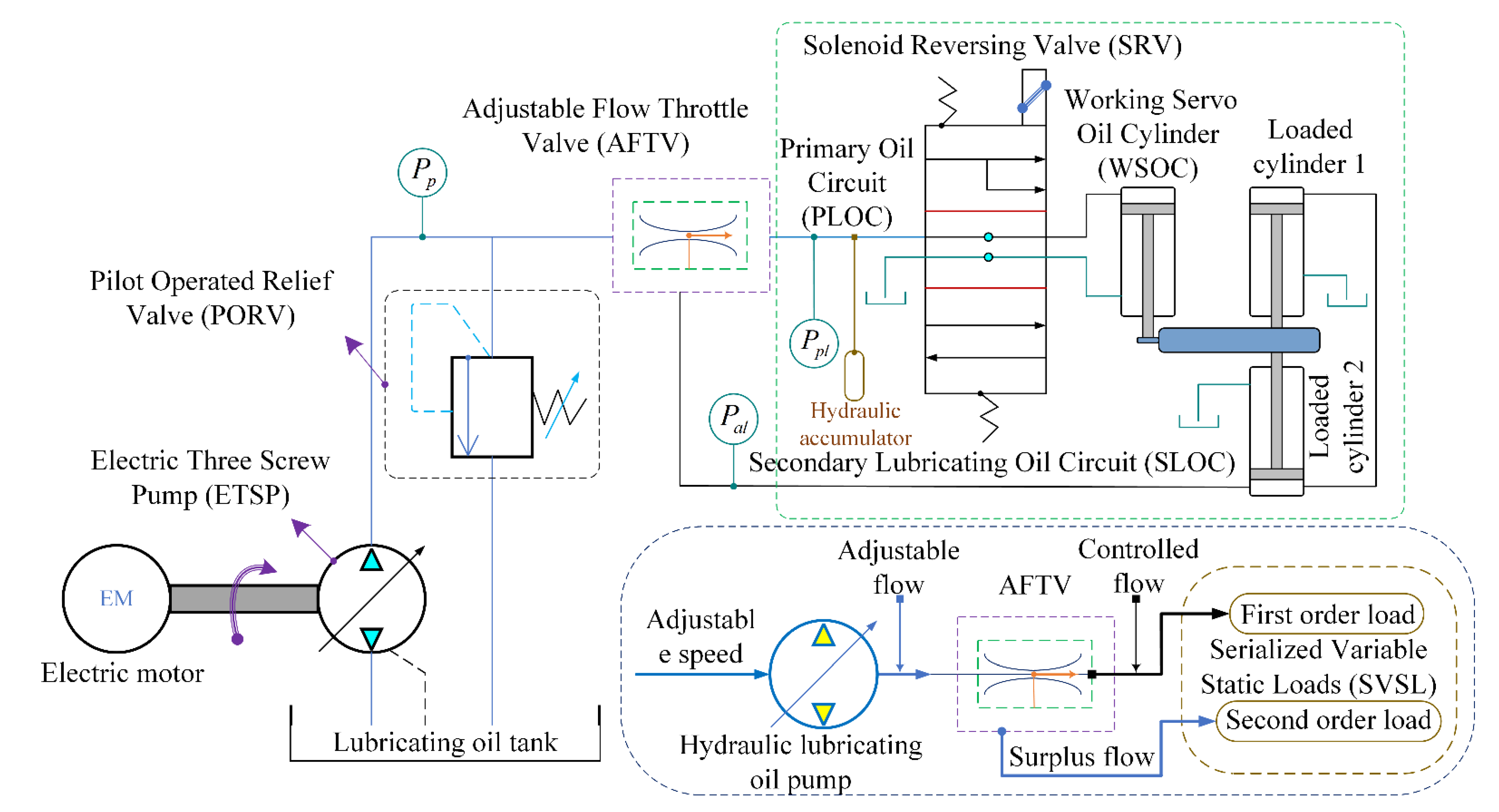
1. Introduction
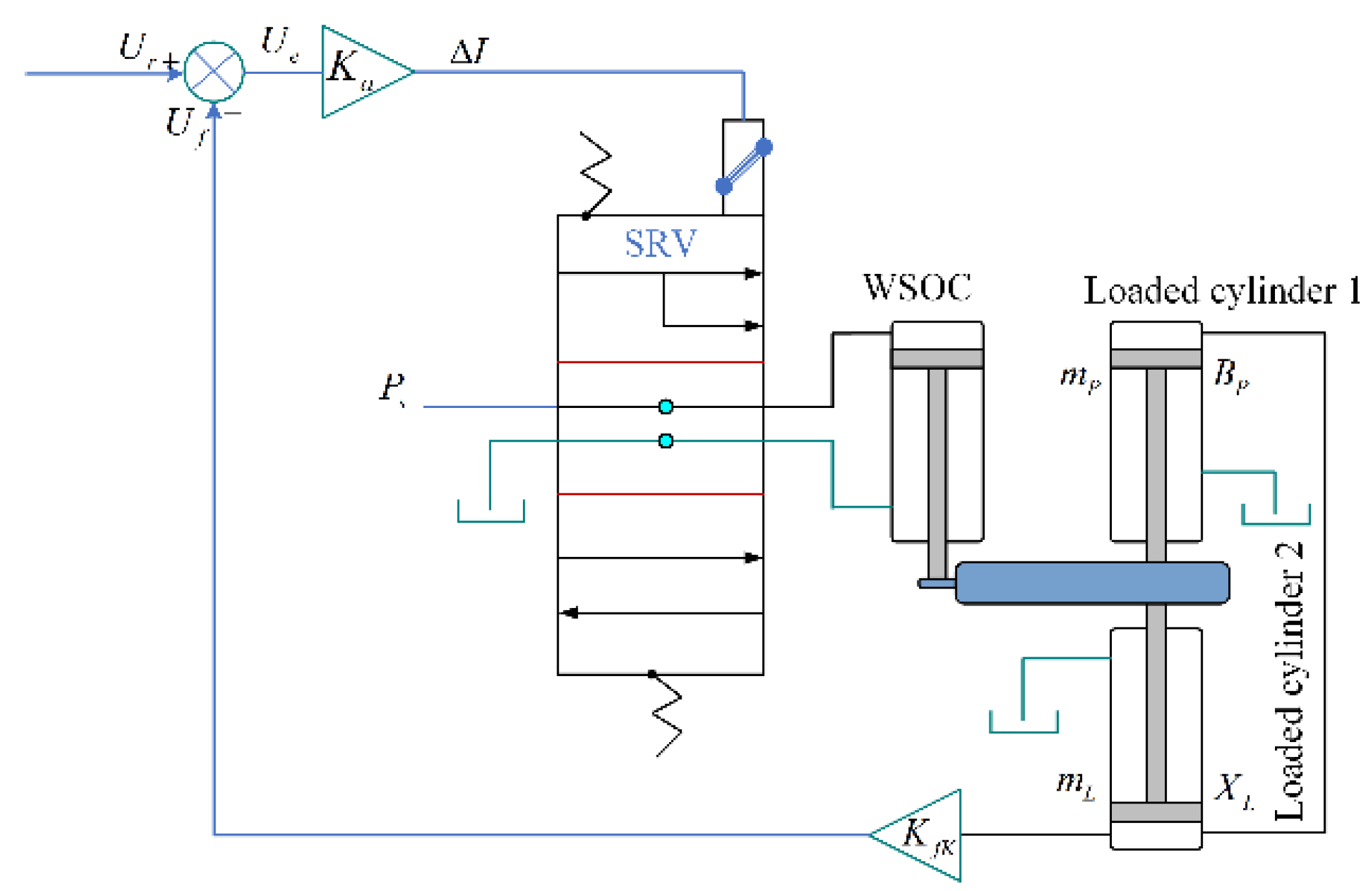
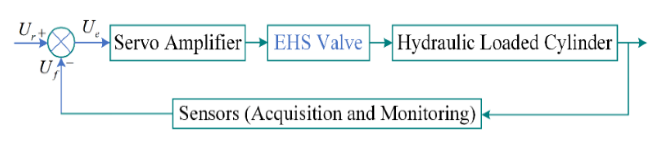
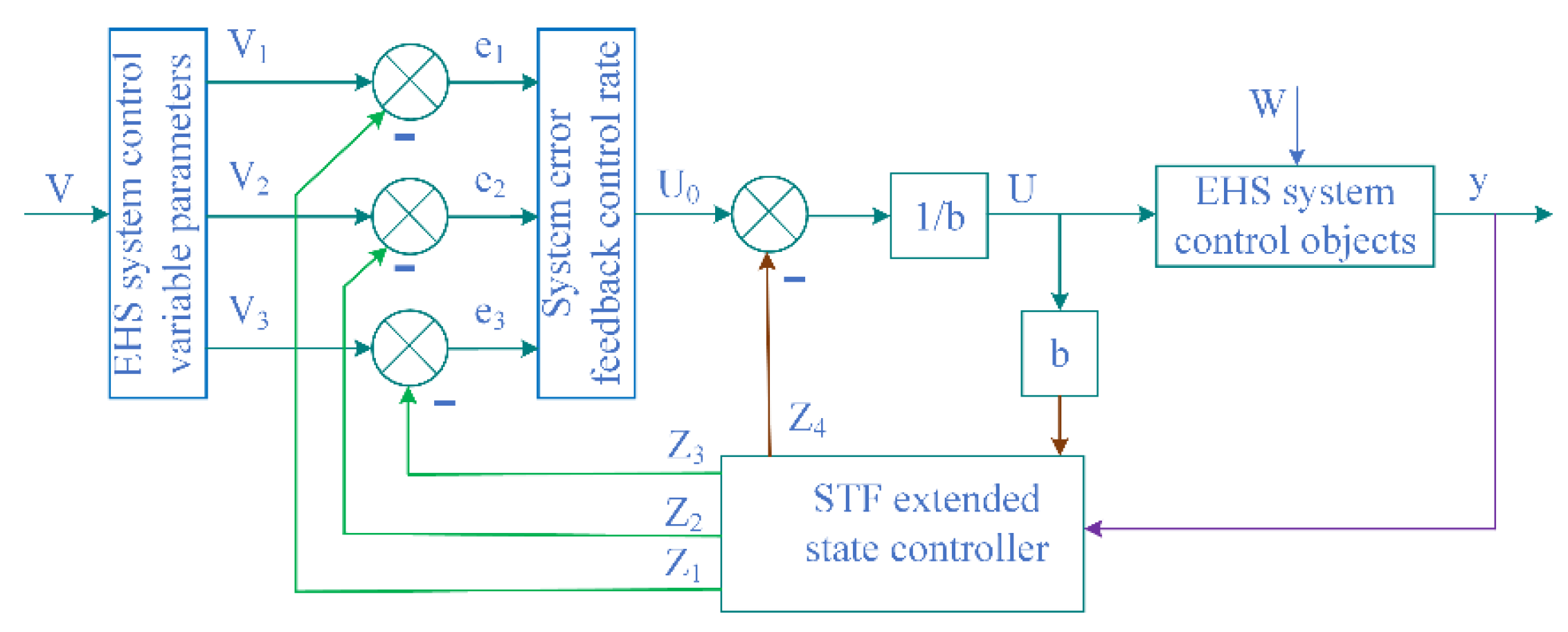
2. EHS Control Modeling of Hydraulic System
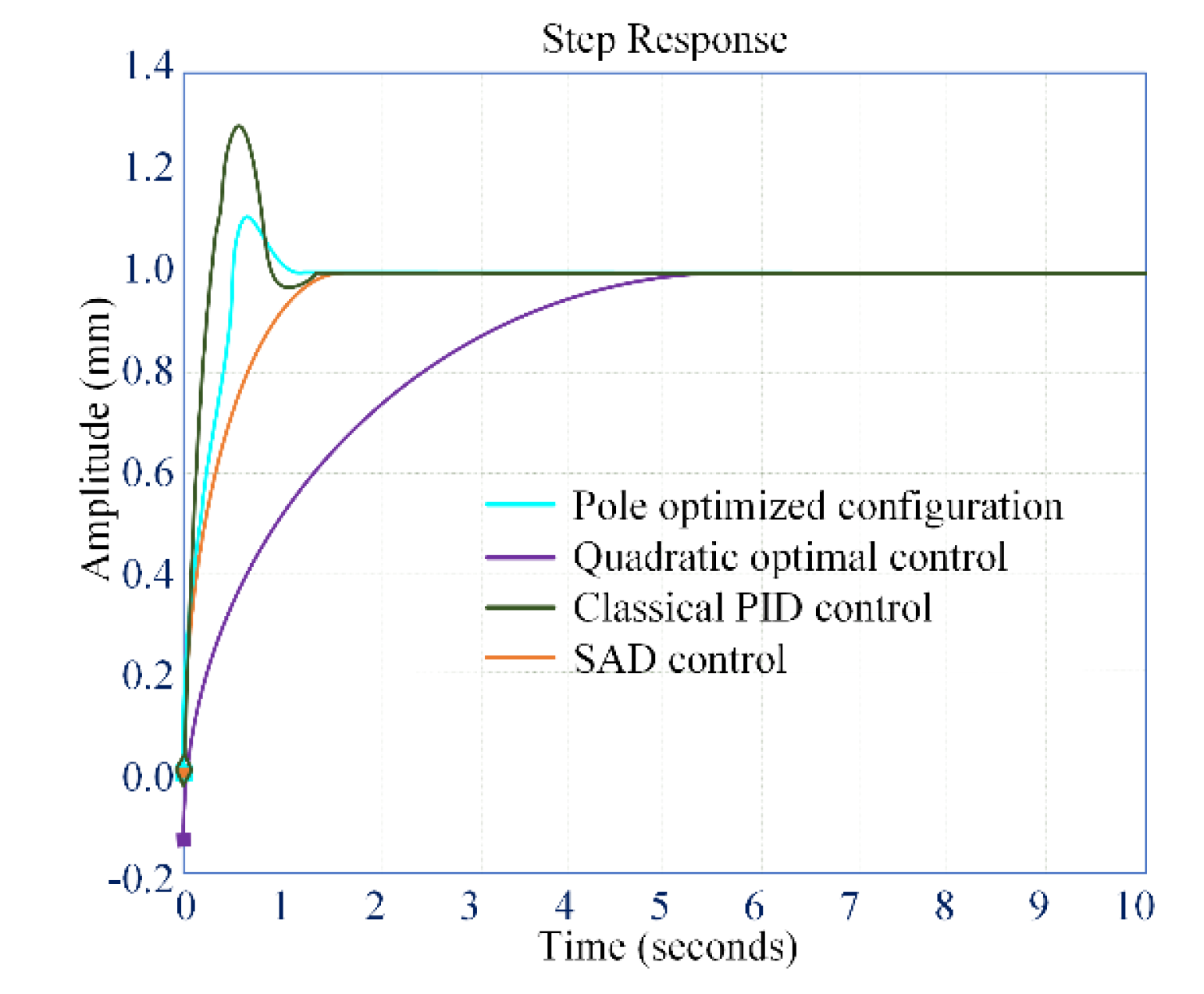
3. Simulation Analysis of Optimal Control Strategy
3.1. Quadratic Optimal Control Analysis with Linearity
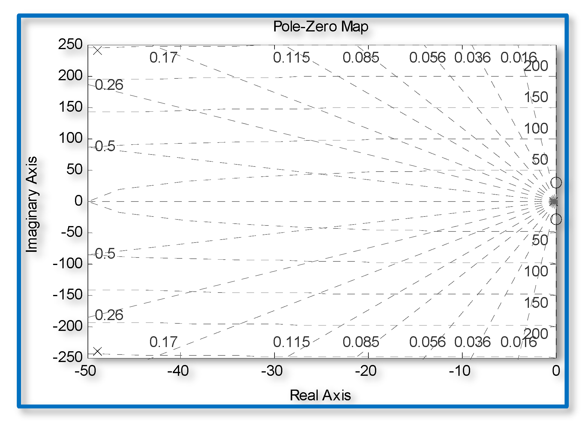
3.2. Pole Optimized Configuration
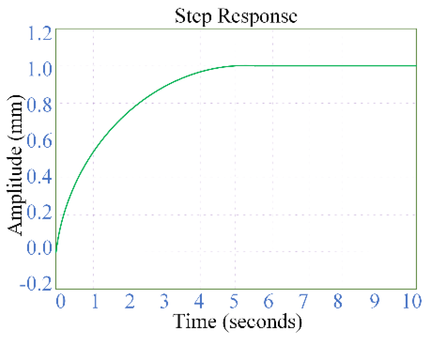
3.3. Simulation Analysis of Classical PID Control
3.4. Simulation Analysis of SAD Control
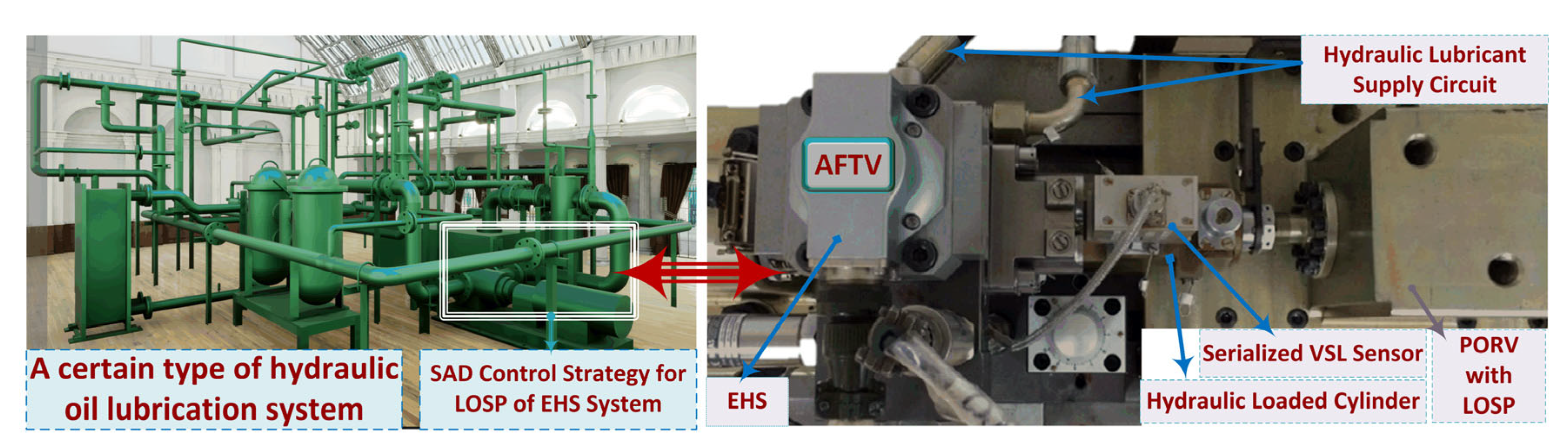
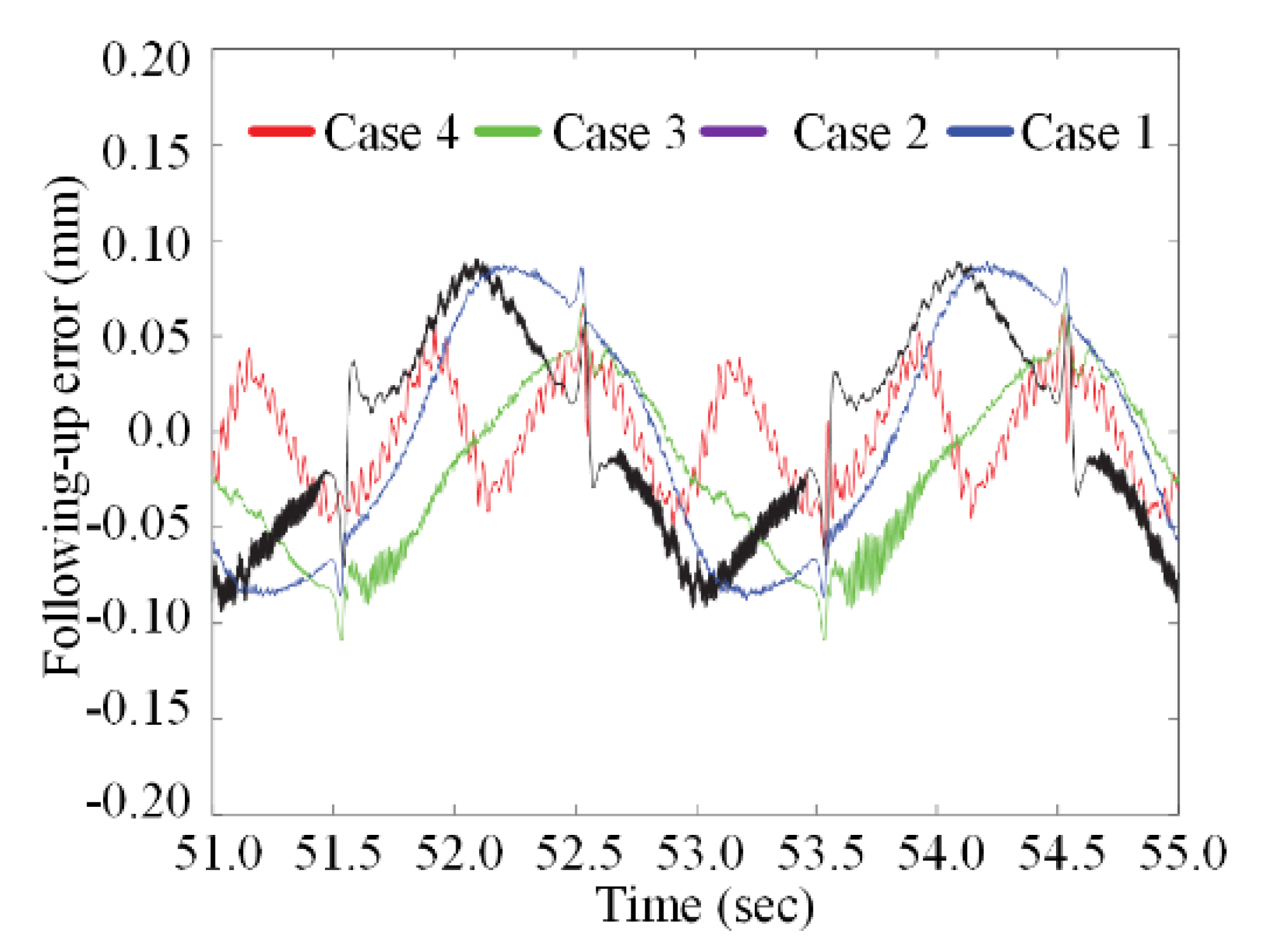
4. Experimental Analysis
5. Discussion of the Results
6. Conclusions
Author Contributions
Funding
Institutional Review Board Statement
Informed Consent Statement
Data Availability Statement
Acknowledgments
Conflicts of Interest
References
- Kumar, S.; Dasgupta, K.; Ghoshal, S.K. Fault diagnosis and prognosis of a hydro-motor drive system using priority valve. J. Braz. Soc. Mech. Sci. 2019, 41. [Google Scholar] [CrossRef]
- Ding, H.; Liu, Y.; Zhao, Y. A new hydraulic synchronous scheme in open-loop control: Load-sensing synchronous control. Meas. Control 2020, 53, 119–125. [Google Scholar] [CrossRef] [Green Version]
- Mahato, A.C.; Ghoshal, S.K. Energy-saving strategies on power hydraulic system: An overview. Proc. Inst. Mech. Eng. Part I J. Syst. Control. Eng. 2021, 235, 147–169. [Google Scholar] [CrossRef]
- Tripathi, J.P.; Hasan, M.; Ghoshal, S.K. Real-time model inversion control for speed recovery of hydraulic drive used in the rotary head of a blasthole drilling machine. J. Braz. Soc. Mech. Sci. Eng. 2022, 44, 1–15. [Google Scholar] [CrossRef]
- Coskun, G.; Kolcuoglu, T.; Dogramacı, T.; Turkmen, A.C.; Celik, C.; Soyhan, H.S. Analysis of a priority flow control valve with hydraulic system simulation model. J. Braz. Soc. Mech. Sci. Eng. 2017, 39, 1597–1605. [Google Scholar] [CrossRef]
- Roemer, D.B.; Johansen, P.; Pedersen, H.C.; Andersen, T.O. Design and modeling of fast switching efficient seat Valve for digital displacement Pump. Trans. Can. Soc. Mech. Eng. 2013, 37, 71–87. [Google Scholar] [CrossRef]
- Zhu, G.; Dong, S.M.; Zhang, W.W.; Zhang, J.J.; Zhang, C. Variable stiffness spring reciprocating pump poppet valves and their dynamic characteristic simulation. China Mech. Eng. 2018, 29, 2912–2916. [Google Scholar]
- Zhong, Q.; He, X.J.; Li, Y.B.; Zhang, B.; Yang, H.Y.; Chen, B. Research on Control Algorithm for High-speed on/off Valves that Adaptive to Supply Pressure Changes. Chin. Mech. Eng. Soc. 2021, 57, 224–235. [Google Scholar]
- Pedersen, N.H.; Johansen, P.; Hansen, A.H.; Andersen, T.O. Model Predictive Control of Low-Speed Partial Stroke Operated Digital Displacement Pump Unit. Model. Ident. Control 2018, 39, 167–177. [Google Scholar] [CrossRef] [Green Version]
- Zhang, B.; Zhong, Q.; Ma, J.E.; Hong, H.C.; Bao, H.M.; Shi, Y.; Yang, H.Y. Self-correcting PWM control for dynamic performance preservation in high speed on/off valve. Mechatronics 2018, 55, 141–150. [Google Scholar] [CrossRef]
- Fan, Y.; Mu, A.; Ma, T. Study on the application of energy storage system in offshore wind turbine with hydraulic transmission. Energ. Convers. Manag. 2016, 110, 338–346. [Google Scholar] [CrossRef]
- Zhu, B.H.; Qian, P.C.; Ji, Z.Q. Research on the flow distribution characteristics and variable principle of the double-swashplate hydraulic axial piston electric motor pump with port valves. J. Mech. Eng. 2018, 54, 220–234. [Google Scholar] [CrossRef]
- Wu, W.P.; Gao, J.J.; Lu, J.G.; Li, X. On continuous-time constrained stochastic linear–quadratic control. Automatica 2020, 114, 108809. [Google Scholar] [CrossRef]
- Ping, Z.W.; Zhou, M.Y.; Liu, C.X.; Huang, Y.Z.; Yu, M.; Lu, J.G. An improved neural network following control strategy for linear motor-driven inverted pendulum on a cart and experimental study. Neural Comput. Appl. 2022, 34, 5161–5168. [Google Scholar] [CrossRef]
- Richiedei, D.; Tamellin, L. Active control of linear vibrating systems for antiresonance assignment with regional pole placement. J. Sound Vib. 2021, 494, 115858. [Google Scholar] [CrossRef]
- Yao, Z.K.; Liang, X.L.; Zhao, Q.T.; Yao, J.Y. Adaptive disturbance observer-based control of hydraulic systems with asymptotic stability. Appl. Math. Model. 2022, 105, 226–242. [Google Scholar] [CrossRef]
- Tan, L.A.; He, X.Y.; Xiao, G.X.; Jiang, M.J.; Yuan, M.J. Design and energy analysis of novel hydraulic regenerative potential energy systems. Energy 2022, 249, 123780. [Google Scholar] [CrossRef]
- Yao, J.Y.; Deng, W.X. Active disturbance rejection adaptive control of hydraulic servo systems. IEEE Trans. Ind. Electron. 2017, 64, 8023–8032. [Google Scholar] [CrossRef]
- Wang, N.; Lin, W.Y.; Yu, J.Y. Sliding-mode-based robust controller design for one channel in thrust vector system with electromechanical actuators. J. Frankl. Inst. 2018, 355, 9021–9035. [Google Scholar] [CrossRef]
- Luo, C.Y.; Yao, J.Y.; Gu, J.S. Extended-state-observer-based output feedback adaptive control of hydraulic system with continuous friction compensation. J. Frankl. Inst. 2019, 356, 8414–8437. [Google Scholar] [CrossRef]
- Palli, G.; Strano, S.; Terzo, M. A novel adaptive-gain technique for high-order sliding-mode observers with application to electro-hydraulic systems. Mech. Syst. Signal Process. 2020, 144, 106875. [Google Scholar] [CrossRef]
- Liu, W.H.; Li, P. Disturbance Observer-Based Fault-Tolerant Adaptive Control for Nonlinearly Parameterized Systems. IEEE Trans. Ind. Electron. 2019, 66, 8681–8691. [Google Scholar] [CrossRef]
- Ye, Y.; Yin, C.B.; Gong, Y.; Zhou, J.J. Position control of nonlinear hydraulic system using an improved PSO based PID controller. Mech. Syst. Signal Process. 2017, 83, 241–259. [Google Scholar] [CrossRef]
- Shi, S.; Xu, X.Y.; Yu, X.; Li, Y.M.; Zhang, Z.Q. Finite-time following control of uncertain nonholonomic systems by state and output feedback. Int. J. Robust Nonlinear Control 2018, 28, 1942–1959. [Google Scholar] [CrossRef]
- Hinderdael, M.; Jardon, Z.; Guillaume, P. An analytical amplitude model for negative pressure waves in gaseous media. Mech. Syst. Signal Process. 2020, 144, 106800. [Google Scholar] [CrossRef]
- Lv, C.; Wang, H.; Cao, D.P. High-Precision Hydraulic Pressure Control Based on Linear Pressure-Drop Modulation in Valve Critical Equilibrium State. IEEE Trans. Ind. Electron. 2017, 64, 7984–7993. [Google Scholar] [CrossRef] [Green Version]
- Mahato, A.C.; Ghoshal, S.K.; Samantaray, A.K. Reduction of wind turbine power fluctuation by using priority flow divider valve in a hydraulic power transmission. Mech. Mach. Theory 2018, 128, 234–253. [Google Scholar] [CrossRef]
- Ba, D.X.; Dinh, T.Q.; Bae, J.; Ahn, K.K. An Effective Disturbance-Observer-Based Nonlinear Controller for a Pump-Controlled Hydraulic System. IEEE/ASME Trans. Mechatron. 2020, 25, 32–43. [Google Scholar] [CrossRef]
- Kumar, S.; Dasgupta, K.; Ghoshal, S.K.; Das, J. Dynamic analysis of a hydro-motor drive system using priority valve. Proc. Inst. Mech. Eng. Part E J. Process Mech. Eng. 2019, 233, 508–525. [Google Scholar] [CrossRef]
- Palli, G.; Strano, S.; Terzo, M. Sliding-mode observers for state and disturbance estimation in electro-hydraulic systems. Control Eng. Pract. 2018, 74, 58–70. [Google Scholar] [CrossRef]
- Razmjooei, H.; Shafiei, M.H.; Palli, G.; Ibeas, A. Chattering-free robust finite-time output feedback control scheme for a class of uncertain non-linear systems. IET Control Theory Appl. 2021, 14, 3168–3178. [Google Scholar] [CrossRef]


Publisher’s Note: MDPI stays neutral with regard to jurisdictional claims in published maps and institutional affiliations. |
© 2022 by the authors. Licensee MDPI, Basel, Switzerland. This article is an open access article distributed under the terms and conditions of the Creative Commons Attribution (CC BY) license (https://creativecommons.org/licenses/by/4.0/).
Share and Cite
Wang, X.; Zhang, J.; Wang, Y.; Li, C. Self-Anti-Disturbance Control of a Hydraulic System Subjected to Variable Static Loads. Appl. Sci. 2022, 12, 7264. https://doi.org/10.3390/app12147264
Wang X, Zhang J, Wang Y, Li C. Self-Anti-Disturbance Control of a Hydraulic System Subjected to Variable Static Loads. Applied Sciences. 2022; 12(14):7264. https://doi.org/10.3390/app12147264
Chicago/Turabian StyleWang, Xigui, Jian Zhang, Yongmei Wang, and Chen Li. 2022. "Self-Anti-Disturbance Control of a Hydraulic System Subjected to Variable Static Loads" Applied Sciences 12, no. 14: 7264. https://doi.org/10.3390/app12147264