Article

Weather Files for the Calibration of Building Energy Models

by
Vicente Gutiérrez González
1,
Germán Ramos Ruiz
1,
Hu Du
2,
Ana Sánchez-Ostiz
1 and
Carlos Fernández Bandera
1,*
1
Department of Building Construction, Services and Structures, School of Architecture, Universidad de Navarra, 31009 Pamplona, Spain
2
School of Architecture, University of Cardiff, Cardiff CF10 3TL, UK
*
Author to whom correspondence should be addressed.
Appl. Sci. 2022, 12(15), 7361; https://doi.org/10.3390/app12157361
Submission received: 29 June 2022 / Revised: 18 July 2022 / Accepted: 19 July 2022 / Published: 22 July 2022

Abstract

:
In the fight against climate change, energy modeling is a key tool used to analyze the performance of proposed energy conservation measures for buildings. Studies on the integration of photovoltaic energy in buildings must use calibrated building energy models, as only with them is the demand curve real, and the savings obtained at the self-consumption level, energy storage in the building, or feed into the grid are accurate. The adjustment process of a calibrated model depends on aspects inherent to the building properties (envelope parameters, internal loads, use schedules) as well as external to them (weather, ground properties, etc.). Naturally, the uncertainty of each is essential to obtaining good results. As for the meteorological data, it is preferable to use data from a weather station located in the building or its surroundings, although this is not always possible due to the cost of the initial investment and its maintenance. As a result, weather stations with public access to their data, such as those located at airports or specific locations in cities, are largely used to perform calibrations of building energy models, making it challenging to converge the simulated model with measured data. This research sheds light on how this obstacle can be overcome by using weather data provided by a third-party company, bridging the gap between reality and energy models. For this purpose, calibrations of the two buildings proposed in Annex 58 were performed with different weather configurations, using the mean absolute error (MAE) uncertainty index and Spearman’s rank correlation coefficient (rho) as comparative measures. An optimal and cost-effective solution was found as an alternative to an on-site weather station, based on the use of a single outdoor temperature sensor in combination with third-party weather data, achieving a robust and reliable building energy model.

1. Introduction

The growing concern to minimize the energy consumption of buildings, associated with climate change mitigation, makes the use of energy modeling increasingly necessary for professionals, designers, architects, and researchers.
The use of building energy modeling is broad; it includes energy certification [1,2,3], the study of energy conservation measures (ECM) [4], fault detection diagnosis (FDD) [5], and the study of complex energy-saving strategies. For the correct quantification of energy-savings in the latter case, the quality and accuracy of the energy model and the weather forecasts are critical. The models must be calibrated, and the weather forecasts must come from reliable sources [6]. In general, these strategies are based on the integration of renewable energies—in particular photovoltaics—into the grid, whether they come from buildings or large energy production centers. Building approaches often derive from the pursuit of nZEB buildings. The challenge in these cases is to try to reduce the period over which the energy balance is measured, generally using monthly or seasonal periods [7,8,9]. D’Agostino et al. analyzed the difference in the sizing of photovoltaic systems (fixed and tracking) when the energy balance was performed on a monthly or annual basis to obtain nZEB buildings [10]. The importance of the energy model is key to demonstrate that if the monthly balance is considered, sometimes the size of the PV plant does not fit the owner’s financial criteria. However, it is not only the energy model that is important; weather forecasting errors can also seriously distort the expected results, leading to significant errors, such as “different energy distributions between heating and cooling’’ [11].
There are also other approaches for self-consumption installations in which the accuracy of the energy model is key to the improvement of the estimation of the building’s energy demand coverage by renewables. There are approaches, such as power-to-heat (P2H), in which the building is used as a thermal battery for the storage of the energy generated hour-by-hour, which allows us to delay it in time so that when heating is needed, it is the building itself that gives it back to us thanks to the fact that it is stored in its thermal inertia [6,12,13,14]; or in model predictive control (MPC) applications, whose objectives are to obtain the optimal heating curve of the building to decide which part of the energy generated is destined for self-consumption and which part of the grid, allowing the optimization of the design of PV self-consumption installations [15,16,17]. All of this can be managed individually or locally by managing the energy balances of the various buildings to make efficient use of the grid by sharing surplus electricity generated on-site [18]. In these cases, the energy model is essential to study both the grid limitation and the storage capacity of the facility [19].
However, several studies report that the results of simulation models in the design phase rarely match the measured performance, calling this deviation, the “energy performance gap” [20]. The possible causes are manifold, ranging from deviations between actual user loads and their predictions, different characteristics of HVAC systems, startups and shutdowns of HVAC systems [21], etc. Regardless of the error of the simulation software itself, the general solution proposed by the researchers to reduce this gap is to use as much real data as possible, from the building characteristics of its envelopes, accuracy when modeling spaces and the environment, and from outside conditions of the building, e.g., the climate [22,23].
To minimize these “discrepancies” and ensure the model’s accuracy, it is advisable to perform a calibration of the energy model. There are numerous strategies used to obtain calibrated models [24] that ultimately attempt to find model parameters that give results that match the measurements obtained. The proper definition of calibration in ASHRAE Standard 14-2014 [25] reads, “process of reducing the uncertainty of a model by comparing the predicted output of the model under a specific set of conditions to the actual measured data for the same set of conditions”. In both this standard and in the International Performance Measurement and Verification Protocol (IPMVP) [26] and in the Federal Energy Management Program (FEMP) [27], uncertainty limits are established, based on the coefficient of the variation of the root mean square error (CV(RMSE)) and the normalized mean bias error (NMBE). These indices limit what is considered a calibrated model and what is not. They are intended to measure the energy uncertainty of the building, but are sometimes also used to measure the deviation between the measured temperature and the temperature generated by the BEM [28,29].
Since the calibration process must be performed taking into account the same indoor and outdoor conditions, the weather file plays an important role in the process. There are three main types of weather files: typical meteorological year (TMY), actual meteorological year (AMY), and weather forecasts. The latter is meaningless in terms of building energy calibration since the main purpose is to perform future predictions on such factors as consumption and comfort; therefore, they need calibrated models to reduce the uncertainty of their predictions, which depend on both the model and the accuracy of the weather forecast.
Typical meteorological year (TMY) weather files are based on meteorological data from previous years—statistically processed—and are intended to represent the location climate. Their suitability depends mainly on the years used for their creation. They are used to obtain the estimated annual energy demand of the building, so that comparative studies, energy certifications, and even consumption calculations can be carried out when generic HVAC systems are used. They are the most common and there is a wide range of repositories of these types of files. These types of weather files do not represent site-specific meteorological conditions and are therefore not recommended for use in calibration processes, as in many cases energy use and peak loads are overestimated or underestimated [30].
Actual meteorological year (AMY) weather files are developed with data from real years without any statistical process. They are used to corroborate the solutions adopted under real climatic conditions. The weather files are necessary to perform calibrations since they provide information on the same “set of conditions” necessary to calibrate [25]. The suitability for the calibration process will largely depend on the origin of the data. There are three possible data sources for the creation of AMY weather files: nearby weather stations, weather data providers, and on-site weather stations. The latter data source will produce the best results, as it will faithfully reproduce the microclimatic conditions of the building under study (heat islands, specific wind speeds, directions conditioned by adjacent buildings, solar radiation conditioned by the environment, etc.). Those coming from data sources from nearby locations (airports, specific places in the city, etc.) may have diametrically opposed microclimatic conditions that do not benefit the calibration process [31]. Finally, those that depend on third-party companies are at the mercy of the accuracy of the algorithms used to interpolate the values of the meteorological variables of the site under study. The general recommendation to reduce the “energy performance gap” involves the use of on-site weather station data [32,33], but this is not always possible due to the high cost of the initial investment and its subsequent maintenance. There is the possibility of using a mixed weather file created from the optimal combination of meteorological variables from external companies and on-site weather stations since not all sensors have the same price, nor do they all have the same impacts in the simulation. This was the main objective of this research.
This research is a continuation of a previous study conducted by the authors in which the impacts of weather files on simulation models were analyzed [34]. Using a previous calibrated model with different AMY weather files from the same location (from an on-site weather station, from a third-party weather company, and all their possible combinations), the impacts on the energy performance gap with respect to the different weather files were analyzed. In this case, the objective of the research was more demanding, since we analyzed the accuracy achieved in the calibration process of a building based on the weather data used, evaluating the use of data from both an on-site weather station and from a third-party weather company, as well as all of their possible combinations, in order to find the most cost-effective one.
To make the results relevant, the degree of calibration of the selected simulation model was important. In this research, the Twin House models analyzed by the International Energy Agency—Energy in Buildings and Communities Programme, IEA EBC Annex 58 “Reliable building energy performance characterization based on full-scale dynamic measurements” [35] were used. The main objective of Annex 58 was to “develop the necessary knowledge, tools, and networks to achieve reliable in situ dynamic testing and data analysis methods that can be used to characterize the actual energy performance of building components and whole buildings”. Different modeling teams (21 in total) were formed to receive the building details and boundary conditions to calibrate the Twin Houses using commercial and research simulation software [36].
The experiment lasted for two months, during which the interior conditions were modified to have different periods of load, free-floating, etc. Therefore, the calibrated model of the Twin Houses developed by the authors was chosen [37]. The calibration methodology used was based on the appropriate selection of capacitances, internal mass, infiltration, and thermal bridges of the model, which allowed obtaining a calibrated model that was one of the first in the ranking of the models obtained by the 21 teams of Annex 58. In this research, the calibrations were carried out using the same methodology, so that it was possible to establish the most cost-effective combination of the AMY weather files in relation to the on-site and third-party weather data used in the calibration process.
The article is structured as follows. Section 2 explains the steps taken to achieve the objectives set out in this paper, the proper simulation and calibration process (Section 2.1), and the weather file creation for the simulations (Section 2.2). Section 2.3 explains the case study used, corresponding to the monitored houses of Annex 58, and the calibration and evaluation periods taken into account. Section 3 shows the results obtained after the simulations and calibrations were performed. Finally, Section 4 presents the conclusions.

2. Methodology

The methodology described below aims to shed light on two problems faced by building energy modelers: (i) the possibility that a BEM can be reasonably matched to reality using a weather file developed with third-party data and (ii) the feasibility of finding a weather file that is best in terms of cost/efficiency, and composed of a combination of data from an on-site weather station and third-party weather
Figure 1 shows a diagram of the different phases of the methodology, indicating in which section each phase is explained.

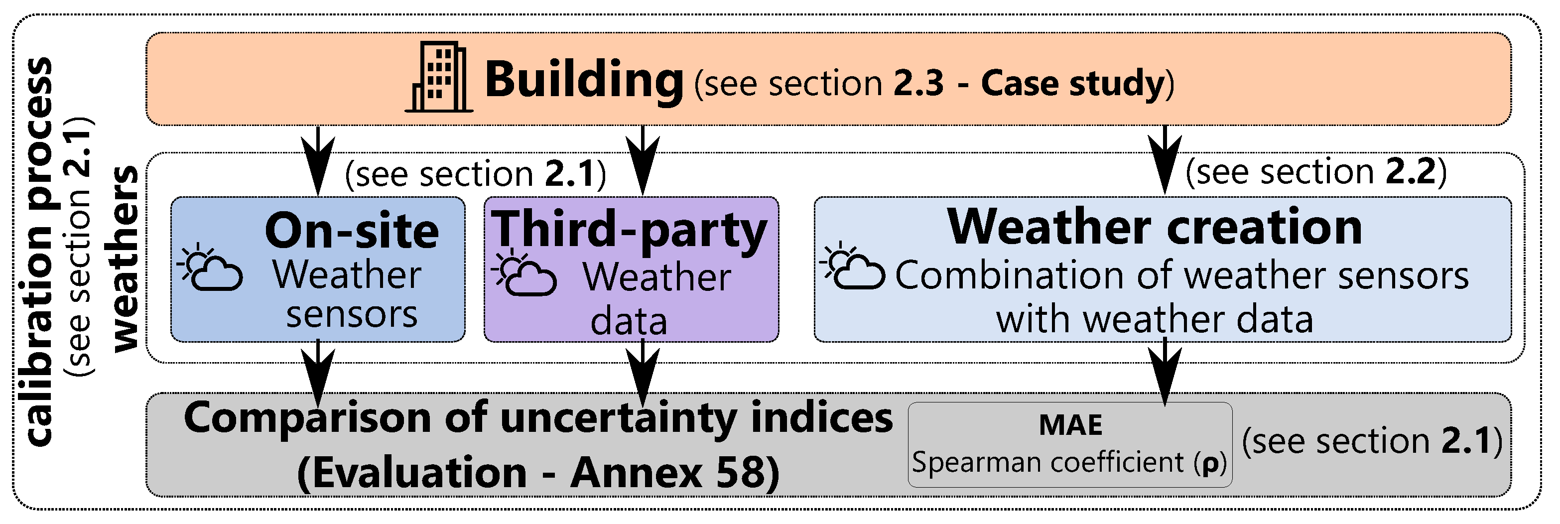
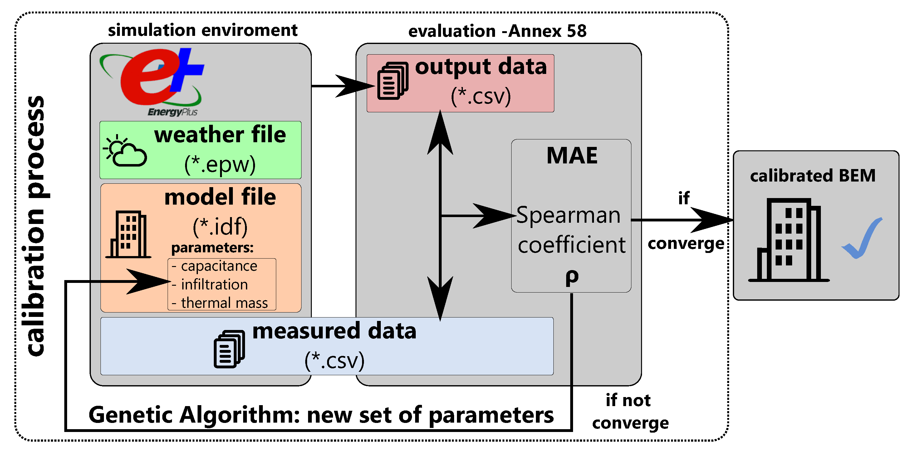
2.1. Calibration Process with On-Site and Third-Party Weather Data

The starting point was an as-built energy model of the building under study, which was the base model on which the calibration process was performed. This first phase of the methodology aimed to analyze the possibility of obtaining optimum quality models using third-party weather files. For this purpose, the BEMs were calibrated with the weather files created with data from the sensors of the on-site weather station and with data from third-party sources during training and checking periods (see Section 2.3).
First, to analyze the differences between the two weather files used, a comparison of their data will be made using the Taylor diagram. In this way, it can be seen quickly and precisely which elements of the two kinds of weather are closer to each other and vice versa (Section 3.1), and make a first evaluation of the impact that each meteorological variable will have on the calibration process.
It is a widely used diagram for weather comparisons [38,39,40,41,42,43], since it shows three statistical metrics in a single figure: the correlation R, the centered root mean square difference ( R M S d i f f ), and the standard deviation between the reference and test values.
The correlation R ranges from 0 to 1, measuring the degree of similarity between two fields, with 1 being the best value. The centered root-mean-squared difference measures its adjustment in terms of amplitude, (the closer to zero means that the patterns are more similar). Both indices provide qualitative and quantitative information, but for complete characterization, it was necessary to know their variances, measured by the standard deviation. All of this information was used to quantify the pattern similarity between two time series (temperature, humidity, direct normal irradiation, diffuse horizontal irradiation, etc.); the closer they were to the center (gray point), the better. As an example (Figure 2), the comparison of the time series represented with the red dot (Example 2) had higher similarity than the one represented with the blue dot (Example 1), reaching a correlation of 0.99 , a standard deviation of 1.175 , and a centered root-mean-square difference of 0.24 . They were virtually identical and, therefore, produced similar results that had a minor impact on the results of the simulations.
σ f 2 = 1 N n = 1 N ( f n f ¯ ) 2
σ r 2 = 1 N n = 1 N ( r n r ¯ ) 2
R = 1 N n = 1 N ( f n f ¯ ) ( r n r ¯ ) σ f σ r
R M S d i f f = 1 N n = 1 N [ ( f n f ¯ ) ( r n r ¯ ) ] 2 1 / 2
After the completion of this first process, both energy models were subjected to the calibration process with the on-site and third-party weather files [37]. The calibration process was performed in a training period and evaluated during a checking period, to avoid possible overfitting of the calibration process.
In order to achieve an energy model adjusted to the real data, the average temperature measured in each of the thermal zones of the building was used to feed the model. This gave the thermal waveform of the real building. The calibration methodology is based on an optimization process using genetic algorithms, whose objective function looks for the relationship between real and simulated data (Figure 3).
The objective function of the optimization performed is based on the uncertainty indices proposed by Annex 58: the mean absolute error (MAE) and the Spearman range correlation coefficient ( ρ ), so that the model obtained could be compared with the models obtained in Annex 58 [45].
  • The mean absolute error (MAE, Equation (5)) between measured ( y i ) and simulated temperatures ( y ^ i ) of each of the thermal zones were calculated to evaluate the difference between them. The results are presented in Section 3.
    M A E = 1 n i = 1 n | y i y ^ i |
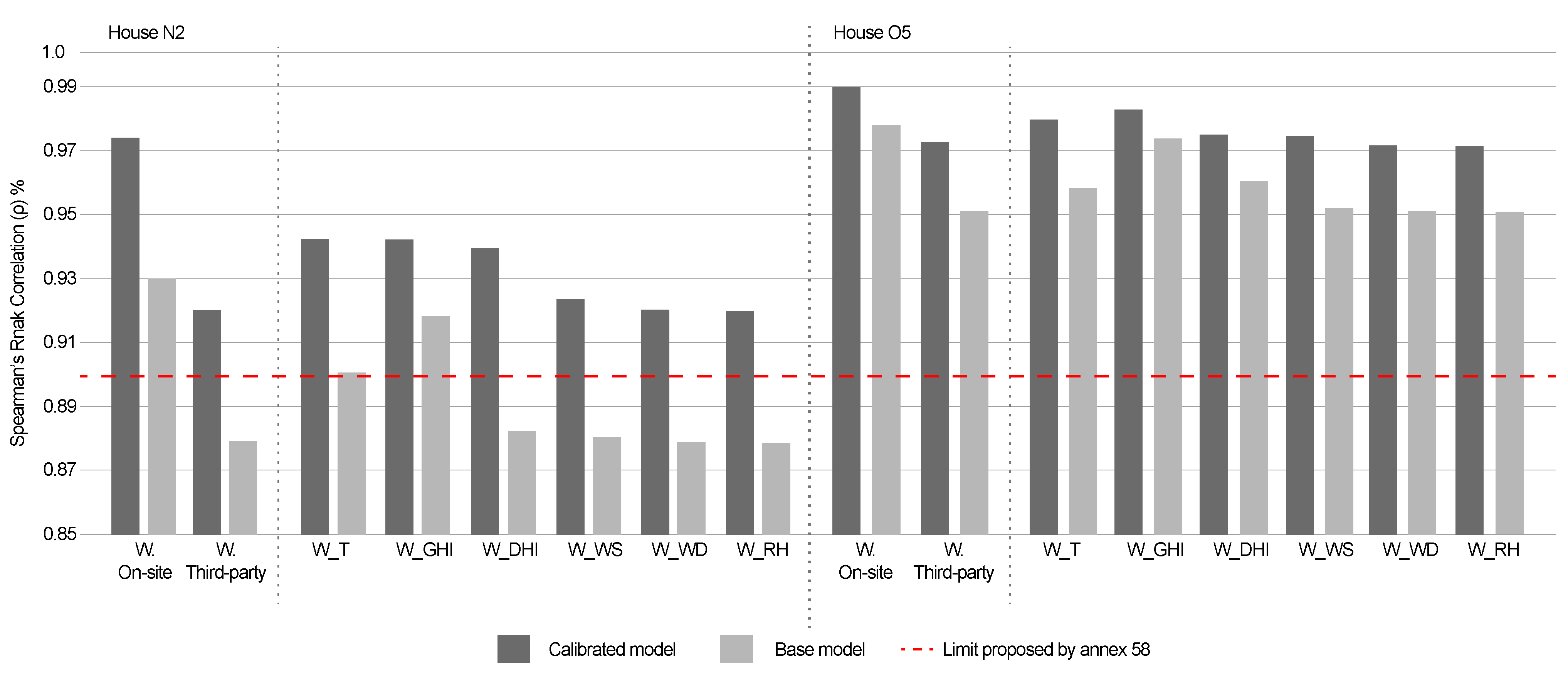
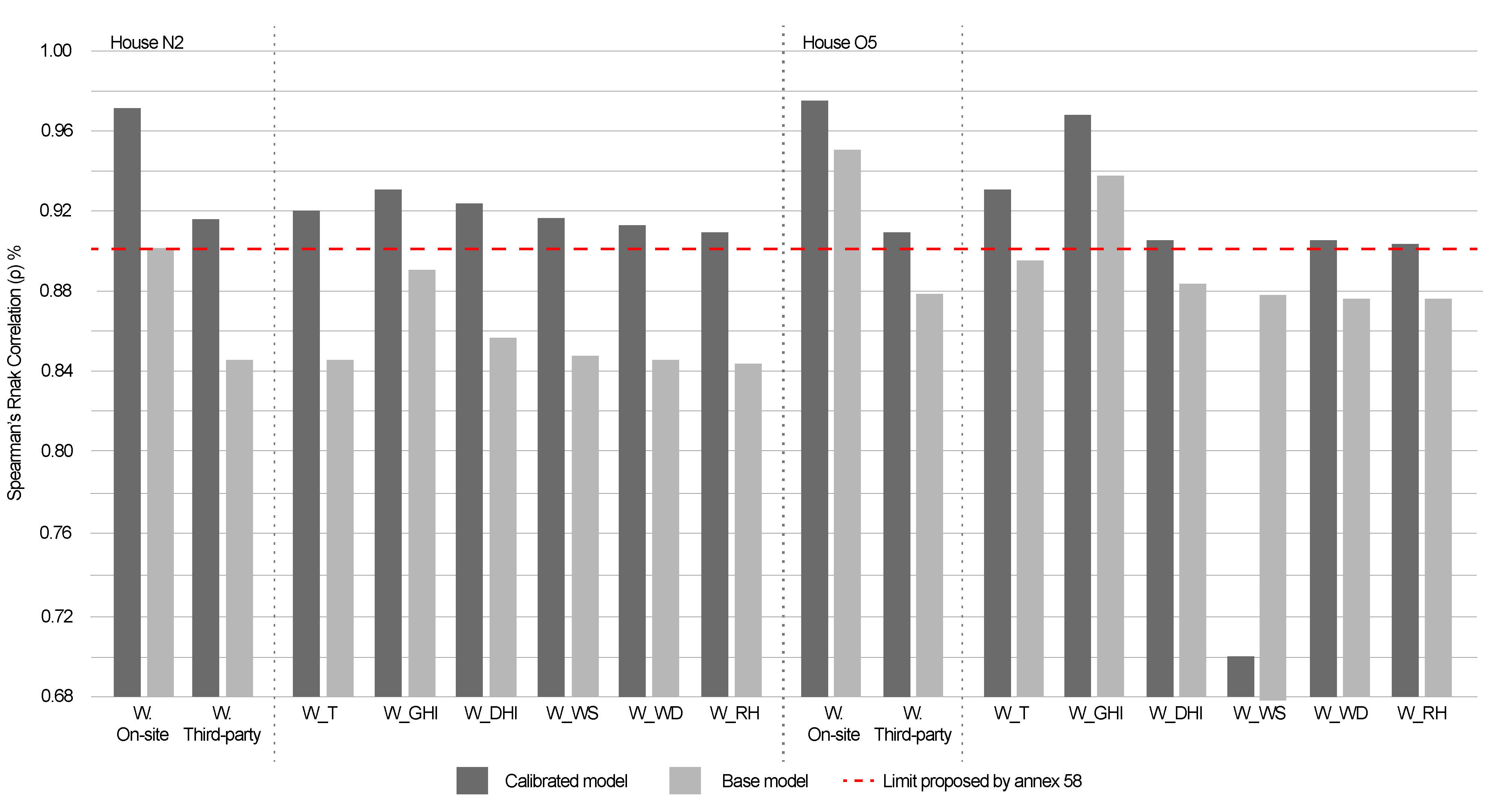
  • The correlation coefficient of Spearman’s range ( ρ , Equation (6)) estimates the level of correspondence of the form. This uncertainty index measures the degree of correspondence that exists between the ranges that are assigned to the values of the analyzed variables.
    ρ = i = 1 n r g ( y i ) r g ( y ) ¯ r g ( y ^ i ) r g ( y ) ¯ i = 1 n r g ( y i ) r g ( y ) ¯ 2 i = 1 n r g ( y ^ i ) r g ( y ) ¯ 2
The non-dominated sorting genetic algorithm (NSGA-II) [46] was chosen to guide these functions towards the optimal result, as it is one of the most widely used algorithms in building optimization strategies [47,48,49]. The proposed combinations for the algorithm to work and, thus, obtain quality results, were based on the parameters of capacitance, thermal mass, and infiltration of each thermal zone (see Figure 3). Once the chosen period has been calibrated according to this methodology, the model that best suits it will be chosen. The calibration process will be repeated with the two proposed weather files (on-site and third-party).
In order to validate the quality of the models, the limits established by Annex 58 were used as a reference, where the BEM was valid if a mean absolute error (MAE) equal to or less than 1 C and a Spearman´s rank correlation coefficient ( r h o ) equal to or greater than 90% were obtained. This is because other standards, such as IPMVP or ASHRAE [26,50], do not give any reference for the evaluation of temperature, but only mention the energy behavior of the BEM. The results are presented in Section 3.2.
Once all of the models were developed, their degrees of fit (with respect to the real data) were analyzed to see whether it was possible to calibrate a BEM using a third-party weather.

2.2. Weather File Creation for the Cost/Effectiveness Analysis
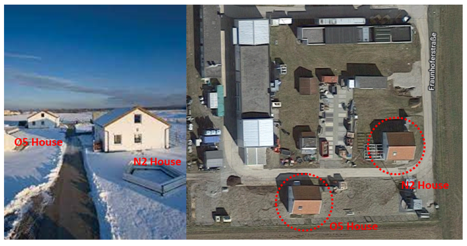
To find out if it was possible to calibrate a building using a weather file composed of a combination of data from an on-site weather station and third-party weather, it was necessary to create each of the possible weather combinations and use them to calibrate the models. In this way, it was possible to analyze which was the best combination in terms of cost/effectiveness. The data from the third-party company were used as the bases for the creation of the weather files, replacing (one by one) all of the meteorological variables measured at the on-site weather station: outside temperature (T), global horizontal irradiation (GHI), horizontal diffuse irradiation (DHI), relative humidity (RH), wind speed (WS), and wind direction (WD). In this way, six weather files were created, as seen in Figure 4.
Once the six new weather files were created, the calibration and evaluation processes were performed for each of them (training and checking periods), taking into account the same limits established in Annex 58 (see Section 3.3), in order to develop the cost/effectiveness analysis.

2.3. Case Study

To implement the methodology proposed in this paper, publicly available data from the Annex 58 IEA-EBC [35,36], Reliable Building Energy Performance Characterisation publication, were adopted. Full-scale dynamic measurements were used for the generation of the energy model and for obtaining the calibrated model. The Annex 58 project started in 2011 and ended in 2016; it was developed with two main objectives: to develop common lines of action that offered improved system performance to obtain energy models, and to achieve quality BEMs capable of reproducing the thermal characteristics of buildings.
Regarding the outcome of the Annex 58 project—a pair of houses (Figure 5), i.e., N2 and O5, located at the test site of the Fraunhofer Institute for Building Physics, Holzkirchen, Germany, was fully monitored with research-grade equipment, and data were made available for the public. Therefore, the Twin Houses were selected in the case studies due to the transparency and the quality of monitoring data.
The houses do not have any elements nearby that could cast a shadow on them in the summer—the season in which the study was carried out. Both houses are located a few meters away from each other. A single weather station was set up for both buildings so that the weather files generated by the on-site sensors were the same for both houses. The station was located about 25 m from N2 and about 45 m from O5. This single station served both houses because it reliably reflected their meteorological environment due to the low density of the site. The recommended distance at which the weather station should be located will be the distance necessary to capture the meteorological characteristics of the building environment. For example, in a high building density environment, such as a large city, the optimal placement of the weather station would be as close to the building as possible, but this distance can be increased if the density decreases and there are no obstacles that make it difficult to clearly obtain the weather characteristics of the building environment.
The buildings are single-family homes with three floors: attic, main floor, and basement. Each has a free height of 2.50 m. The study focused on the main floor, as was done in the project described in Annex 58. The main floor has a configuration of two bedrooms, a corridor, a bathroom, a kitchen, a living room, and an entrance.
The monitoring conducted in Annex 58 involved five periods (Table 1) in terms of thermal dynamic characteristics to reflect the common conditions of the buildings. Each period had bespoke configurations, and the BEM must have been capable of responding to reality in terms of the energy consumed and the temperature reached. The proposed period began with the first (initialization), lasting three days, in which a constant interior temperature of 30 C was maintained in the buildings. In period 2, with a seven-day duration, a constant temperature of 30 C was maintained inside the houses. In period 3, which lasted 14 days, the energy was introduced through the living room radiator at random periods with a randomly ordered logarithmic binary sequence (ROLBS). This sequence was created in the EC COMPASS project . Its goal was to give the same influence to all energy inputs that affected the BEM. The energy inputs and the free oscillation intervals were selected so that they did not stand out from each other and were mixed in a quasi-random way. Using this form of introducing power into the models, there is no relationship between the energy introduced by the HVAC systems (or heating system) and the solar energy. The energy model must be able to reproduce the internal temperature that this energy produces. In period 4, a constant temperature was again introduced into the houses, but this time at 25 C. In the last period (period 5), where the house was left in free oscillation without any energy input, the model trued to reproduce the interior temperatures.
Two of the five periods proposed in Annex 58 were used to conduct the study in this paper. Period 3 (ROLBS) was chosen as the training or calibration period, which ran from 30 August to 14 September 2013, since the random load of the living room radiator, by heat pulses of 500 W, governed by the randomly ordered logarithmic binary sequence, allowed the optimization algorithm to find solutions that properly captured the thermal dynamics of the building. The evaluations of the energy models were performed in period 5 (checking) from 20 to 30 September 2013, where the buildings were not subjected to any load from equipment or people. It was the best period to verify that the model obtained had captured the thermal dynamics of the building. Different and non-consecutive calibrations and checking periods were chosen to ensure that the experiment was free from the effect of overfitting inherent to the calibration process.

3. Results and Discussion

3.1. Comparison of In Situ and Third-Party Weather Files

The first elements to be analyzed and evaluated were the weather files used in the simulations. For this purpose, the Taylor diagram [51,52] was used to see which weather parameters were similar and which were not, so that it was possible to predict which of them would have better behavior.
Figure 6 shows the comparison of the two weather files. Both are the actual meteorological year (AMY) generated with the information of the on-site weather station and a third-party. As can be seen, there were large differences in wind speed and wind direction, which influenced both the baseline and the calibrated model.
According to the results obtained and shown in the diagram, the temperature and diffuse radiation data were the most similar to the ones provided by the on-site weather station, while the least similar were those related to the wind (direction and speed).
The following subsections show the results of the model simulations and calibrations using on-site and third-party weather, as well as the combinations of both to obtain more cost-effective weather data.

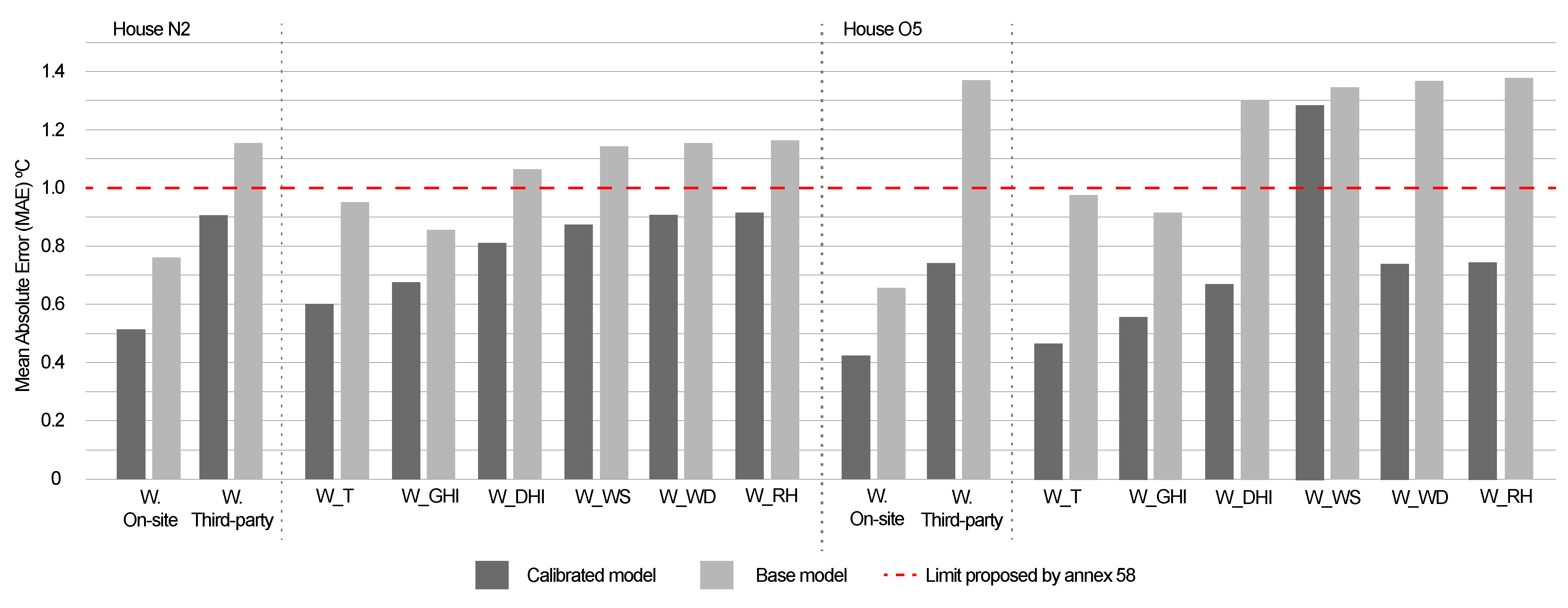
3.2. Simulation and Calibration Results: On-Site vs. Third-Party Weather Data

Table 2 shows the results of both the base model and the model obtained after the calibration process of the two case studies: N2 and O2 houses. The weather files used were developed using the on-site and third-party weather data during the training and checking periods. The left side of the table shows the housing (N2 or O5); the model (base or calibrated); the type of weather file used, and the simulation period. The right side shows the adjustment results obtained by the thermal zone, following the same scheme proposed in Annex 58. Finally, the adjustment is presented; we performed an area-weighted average of the thermal zones involved in the process (global index). The results (MAE and ρ ) are subdivided by columns highlighted in red showing the ones that exceed the limits proposed by Annex 58.
The first result to highlight in Table 2 is that all the models (base and calibrated) that used the on-site weather file were within the acceptable limits proposed by Annex 58. The calibrated models have a better fitting.
When looking at the results produced by the third-party weather file, the base models did not comply with the acceptable limits in either house. Their global indices were far from these limits, both in the training period and in the checking period (marked in red), except for one parameter in the O5 house during the training period, whose ρ index reached 95.0%. This result reinforces the need to use calibrated models for complex energy-saving strategies, such as P2H solutions, MPC applications, etc.
On the other hand, when calibrated models from both houses were used, all the weather files (third-party and on-site) were within the proposed limits. Therefore, the calibration process not only makes better use of the indoor data but also overcomes errors in the environmental sensors. This way, a third-party weather file could be considered an option for improving models with an acceptable error index. The fact that the same results were achieved in two different models and that both were checked in an independent period shows that they are robust and avoid the risk of overfitting in the solutions.
Table 2 also shows the results obtained in the thermal areas that were analyzed. These thermal zones are the same as those proposed in the project of Annex 58. In general, it is observed that the models that underwent the calibration process generated a better fit with the real data than the base models. Therefore, when the thermal zones were analyzed individually, they followed the same pattern as when the global data of the houses were analyzed: the calibration process helped the model approach the limits set by Annex 58, making the use of a third-party weather file feasible.

3.3. Simulation and Calibration Results: Combination of On-Site and Third-Party Weather Data

Table 3 and Table 4 show the simulation results of the base and calibrated models in the training and checking periods, respectively. The studies were performed using the weather files created by the on-site weather station, third-party weather, and the combination of data proposed in Section 2.2. In order to facilitate its understanding, only the global MAE index of both models is shown. The rest of the results by the thermal zone, globally, as well as the ρ index obtained, are shown in Appendix A.
The results shown in Table 3 (training period) are homogeneous. All the models, when submitted to the calibration process, managed to improve their indices with respect to their base models. The range of improvement was between 30% and 39% in the case of N2, and 45% and 55% in the case of O5. Secondly, the base model was beyond the limits with all the combined weather files (values in red), except the on-site weather. This result strengthened the first goal of this research, which was to show how the calibration process could overcome faulty environmental data. In this case, as both models were trained during this period, the overfitting could be an argument against this result.
Focusing on the new weather files, some improved the results of the base model simulated with the third-party weather files; these were: Weather_T; Weather_GHI and Weather_DHI. The weather files weather_WS, weather_WD, and undefined weather_RH slightly improved or worsened the results.
Regarding the results obtained by the calibrated models, all of them can be considered quality models, since they comply with the limits recommended by Annex 58. Regarding the improvement produced by the sensors when the data from the on-site weather station entered into the weather file of a third-party, the same effects were produced as in the base models. The weather files weather_T, weather_GHI, and weather_DHI, in both houses, considerably improved the adjustment produced by the model calibrated with the weather file generated with the data of the third party. The models calibrated with weather_WS, weather_WD, and weather_RH improved very little or even worsened the results.
Table 4 shows the results achieved when considering the base and the calibrated models in the checking period. These were very similar to those obtained during the training period, but in this case, there was no risk of overfitting because the data were independent of the training period.
When the base models were simulated with the different weather files, only three of them complied with the limits suggested by Annex 58: the models simulated with weather files weather_T and weather_GHI and the on-site data. The others did not meet the expectations (marked in red). However, when these models underwent the calibration process, they all improved their indices, introducing them within the range set out in Annex 58.
When examining the effects of the sensors, as it happened during the training period, there was a group of sensors that generated weather files that improved the adjustment produced by the third-party data in both models—based and calibrated—these files were: weather_T, weather_GHI, and weather_DHI. The weather files weather_WS, weather_WD and weather_RH showed very little improvement and even worse when their results were compared with the models simulated with the third-party weather file.
Looking at Table 4 (O5 house), one can see how an anomalous result was produced in the model calibrated with the weather file weather_WS. The result produced by the MAE index was much higher than the rest of the models, and could not be placed within the limits of Annex 58. This can be considered an outlier, as it does not apply to the rest of the tests performed. This result complies with that obtained after the comparative analysis of the weather files in the Taylor diagram (see Figure 6).
One aspect that should be highlighted when looking at the results is that, for the two houses, and in both periods, there was a correlation between the improvement produced by the new weather files in the base models and that of the calibrated models. This correlation reached 95% for the two houses in the training period and 92% for the testing period. Looking at the results obtained, it could be concluded that, if there was a significant improvement in the degree of fit with the new weather file with respect to the third-party file, this will also occur if the model is subjected to a calibration process. This effect could be used as a prior qualitative test before carrying out the calibration process, which is costly in time. It should also be taken into consideration that the range of improvement between the based and calibrated models is not the same, and some discrepancies can occur.
To summarize, Figure 7 and Figure 8, respectively, produce a general view of the whole process, the results of which are discussed in the tables above. The dark grey bars represent the calibrated models, while the light grey bars represent the base models, which have not undergone any calibration process. The red dotted line indicates the limit imposed by Annex 58 to judge the quality of the model. When the models are below this line in the MAE index, they meet the quality conditions set.
The effects of the calibration process and the different types of weather files on the energy models were also measured with the ρ index. Figure 9 and Figure 10 show the ρ indices obtained by the different models when they were simulated and calibrated with the new weather files in the training and checking periods for both houses, as quantitatively shown in the tables described above. As in Figure 7 and Figure 8, the light grey represents the model that was not subjected to any calibration process (base model), while the dark grey shows the results of the models that underwent the calibration process (calibrated model). The red dotted line shows the limit of Annex 58 to indicate the quality of the model. When the model exceeds that line, it is considered to be of quality.

4. Conclusions

The integration of renewable energies (particularly photovoltaic) in buildings for the study of complex energy-saving strategies, such as power-to-heat (P2H) or model predictive control (MPC), depends on the quality/accuracy of the energy models and weather forecasts. One of the key challenges in developing these realistic energy models is dealing with the many uncertainties involved in the process. Obtaining accurate building information is essential to developing a robust simulation model, but it is often a complex task. Weather data are part of this information and the quality will have a major influence on the results obtained.
An on-site weather station requires a heavy financial investment, not only in buying or renting the necessary sensors but also in processing and validating the generated data. They often have to be placed by expert personnel in order for these sensors to collect the data as realistically as possible, without interference from external factors. Despite these drawbacks, the data generated by these stations are optimal for input into an energy model calibration process.
An alternative to the on-site weather station is the use of data from a third-party weather company. This is much cheaper and requires no effort to collect, but its major disadvantage is that it is generally much less accurate. BEMs simulated with the weather files provided by a third-party are much further away from the real building (when analyzing the behavior) than those simulated with the data provided by the on-site weather station. However, if these inputs are subjected to a calibration process, it is possible to obtain quality models that meet established objectives. This makes it feasible to use these files as a better alternative than using data from weather stations that do not take into account the characteristics of the building under study (weather stations located at airports or in specific places in the city).
Although data provided by on-site weather station sensors continue to provide the best results in model fitting, this study has shown that third-party data are viable when the BEM is subjected to a calibration process, creating an alternative when choosing a weather file. In turn, the solution that could be the best (in terms of cost/effectiveness and efficiency) was found—the archive combining third-party weather data and outdoor temperature data measured in situ. This possibility is of great relevance as it allows obtaining calibrated models of buildings where a BMS with historical indoor and outdoor temperature data are available. Nowadays, these types of models are in great demand as they provide very useful information in optimization strategies that require training with data, such as machine learning, artificial neural networks, etc.
One relevant finding obtained in this study is that it is possible to know in advance which sensors of the in situ weather station, when introduced into the data of a third-party weather file could improve the fit data of the calibrated model without being subjected to this adjustment process. The concordance results obtained with the simulation of the base model and the different weather files are proportionally similar to those obtained when the model is subjected to the calibration process.
In the future, more case studies with different building characteristics, such as orientation, window wall ratio, thermal fabric properties, and weather conditions, should be explored to confirm these findings.

Author Contributions

Conceptualization, V.G.G., C.F.B. and G.R.R.; methodology, V.G.G. and C.F.B.; software, V.G.G. and G.R.R.; validation, V.G.G., C.F.B. and G.R.R.; formal analysis, V.G.G.; investigation, V.G.G.; resources, V.G.G.; data curation, V.G.G.; writing—original draft preparation, V.G.G.; writing—review and editing, V.G.G., G.R.R., C.F.B., H.D. and A.S.-O.; visualization, V.G.G. and G.R.R.; supervision, C.F.B. All authors have read and agreed to the published version of the manuscript.

Funding

This research was funded by the Government of Navarra under the project “From BIM to BEM: B&B” (ref. 0011-1365-2020-000227).

Institutional Review Board Statement

Not applicable.

Informed Consent Statement

Informed consent was obtained from all subjects involved in the study.

Data Availability Statement

Not applicable.

Acknowledgments

We would like to thank the promoters of Annex 58 for access to the data of the houses. Without these data, it would not have been possible to complete this work.

Conflicts of Interest

The authors declare no conflict of interest.

Abbreviations

The following abbreviations are used in this manuscript:
AMYactual meteorological year
BEMbuilding energy models
CV(RMSE)coefficient of variation of root mean square error
DHIdiffuse horizontal irradiation
ECMenergy conservation measures
FEMPfederal energy management program
FDDfault detection diagnosis
GHIglobal horizontal irradiation
IPMVPinternational performance measurement and verification protocol
MAEmean absolute error
MPCmodel predictive control
NMBEnormalized mean bias error
NSGA-iinon-dominated sorting genetic algorithm
P2Hpower to heat
RHrelative humidity
ROLBSrandomly ordered logarithmic binary sequence
TMYtypical meteorological year
WDwind direction
WSwind speed

Appendix A. Complementary Data from the Base and Calibration Processes by the Thermal Zone, with the Different Weather Files

Table A1Table A8 show the results obtained in each house by the thermal zone, both by the base and calibrated models, when simulated with the different types of weather files in the training and checking period.
The thermal zones evaluated correspond to those indicated in Annex 58. Those that do not reach the quality index set out are marked in red.
Table A1. MAE and ρ indices per thermal zone in the training period. House N2, base model.
Base
Model
Weather File
Name
Simulation
Period
Living
Room
Children
Room
BedroomKitchenGlobal
Index
MAE ( C) ρ (%)MAE ( C) ρ (%)MAE ( C) ρ (%)MAE ( C) ρ (%)MAE ( C) ρ (%)
N2On-siteTraining1.5496.60.2598.60.5097.20.9796.50.8193.0
N2Third-partyTraining1.2194.90.6699.11.1694.72.5790.51.4087.9
N2Weather_TTraining1.3295.70.3998.60.8196.02.0992.41.1588.2
N2Weather_GHITraining1.2795.50.6199.31.1493.71.3894.41.1091.8
N2Weather_DHITraining1.1195.50.5999.00.9097.12.2792.91.2290.0
N2Weather_WSTraining1.2194.90.6499.11.1394.72.5390.61.3888.0
N2Weather_WDTraining1.2194.90.6699.11.1694.72.5790.51.4087.9
N2Weather_RHTraining1.2194.90.6799.11.1794.72.5990.51.4187.8
Table A2. MAE and ρ indices per thermal zone in the checking period. House N2, base model.
Base
Model
Weather File
Name
Simulation
Period
Living
Room
Children
Room
BedroomKitchenGlobal
Index
MAE ( C) ρ (%)MAE ( C) ρ (%)MAE ( C) ρ (%)MAE ( C) ρ (%)MAE ( C) ρ (%)
N2On-siteChecking1.8291.90.2299.60.3298.30.6595.50.7590.1
N2Third-partyChecking0.84687.50.7399.40.9397.22.0986.21.1584.5
N2Weather_TChecking1.2390.30.4199.50.5797.01.5789.10.9584.5
N2Weather_GHIChecking1.0988.30.5999.40.8197.20.9290.90.8588.9
N2Weather_DHIChecking0.7988.90.6999.60.7898.61.9887.81.0685.6
N2Weather_WSChecking0.8487.60.7299.40.9297.32.0886.41.1484.6
N2Weather_WDChecking0.8487.50.7399.40.9397.22.0986.31.1584.5
N2Weather_RHChecking0.8487.40.7499.40.9497.12.1186.11.1684.4
Table A3. MAE and ρ indices per thermal zone in the training period. House N2, calibrated model.
Calibrated
Model
Weather File
Name
Simulation
Period
Living
Room
Children
Room
BedroomKitchenGlobal
Index
MAE ( C) ρ (%)MAE ( C) ρ (%)MAE ( C) ρ (%)MAE ( C) ρ (%)MAE ( C) ρ (%)
N2On-siteTraining0.5698.60.4198.20.4496.80.7995.130.5597.4
N2Third-partyTraining0.9896.20.4299.00.7792.01.7390.20.9892.0
N2Weather_TTraining0.6896.70.2598.00.5494.61.2992.50.6993.6
N2Weather_GHITraining0.8596.70.4099.10.7991.20.9793.40.7594.2
N2Weather_DHITraining0.8796.80.3698.90.6095.31.4692.70.8294.2
N2Weather_WSTraining0.9696.10.3699.00.7692.11.6390.70.9392.3
N2Weather_WDTraining0.9896.20.4299.00.7792.01.7390.20.9892.0
N2Weather_RHTraining0.9896.20.4399.00.7892.01.7490.20.9891.9
Table A4. MAE and ρ indices per thermal zone in the checking period. House N2, calibrated model.
Base
Model
Weather File
Name
Simulation
Period
Living
Room
Children
Room
BedroomKitchenGlobal
Index
MAE ( C) ρ (%)MAE ( C) ρ (%)MAE ( C) ρ (%)MAE ( C) ρ (%)MAE ( C) ρ (%)
N2On-siteChecking0.3299.70.6099.90.3898.80.7493.70.5197.1
N2Third-partyChecking0.4994.00.7299.50.8297.81.5885.60.9091.5
N2Weather_TChecking0.7896.50.4099.60.4697.81.0488.70.6092.1
N2Weather_GHIChecking1.0994.80.5999.50.8197.80.9190.20.8593.2
N2Weather_DHIChecking0.7994.70.6899.40.7898.91.9887.11.0692.2
N2Weather_WSChecking0.8494.10.7299.40.9297.72.0885.91.1491.8
N2Weather_WDChecking0.8494.00.7499.50.9397.82.0985.61.1591.6
N2Weather_RHChecking0.8494.00.7499.50.9497.72.1185.51.1691.5
Table A5. MAE and ρ indices per thermal zone in the training period. House O5, base model.
Base
Model
Weather File
Name
Simulation
Period
Living
Room
Children
Room
BedroomKitchenGlobal
Index
MAE ( C) ρ (%)MAE ( C) ρ (%)MAE ( C) ρ (%)MAE ( C) ρ (%)MAE ( C) ρ (%)
O5On-siteTraining1.4698.70.6098.70.2898.60.4898.40.7197.8
O5Third-partyTraining2.1095.91.2698.10.8296.01.8393.31.5095.0
O5Weather_TTraining1.6796.51.0098.10.5196.71.3795.01.1495.8
O5Weather_GHITraining1.9197.71.2399.10.8295.30.9895.91.2497.4
O5Weather_DHITraining1.8396.51.1698.10.5898.71.5594.81.2896.0
O5Weather_WSTraining2.0796.01.2298.10.7896.01.7693.41.4695.1
O5Weather_WDTraining2.1096.01.2698.10.8296.01.8393.31.5095.1
O5Weather_RHTraining2.1196.01.2798.10.8396.01.8493.21.5195.0
Table A6. MAE and ρ indices per thermal zone in the checking period. House O5, base model.
Base
Model
Weather File
Name
Simulation
Period
Living
Room
Children
Room
BedroomKitchenGlobal
Index
MAE ( C) ρ (%)MAE ( C) ρ (%)MAE ( C) ρ (%)MAE ( C) ρ (%)MAE ( C) ρ (%)
O5On-siteChecking1.3197.90.5499.70.2697.40.5096.90.6595.0
O5Third-partyChecking1.6884.41.4397.80.7094.01.6488.21.3687.7
O5Weather_TChecking1.1686.91.1698.60.4194.81.1592.00.9789.5
O5Weather_GHIChecking1.2894.71.0998.90.5993.90.6891.40.9193.8
O5Weather_DHIChecking1.6484.11.4498.00.5797.61.5390.01.3088.6
O5Weather_WSChecking1.6684.51.4197.90.6994.21.6188.51.34687.9
O5Weather_WDChecking1.6884.41.4497.80.7094.01.6488.21.3687.7
O5Weather_RHChecking1.7084.41.4497.80.7193.91.6688.11.3787.7
Table A7. MAE and ρ indices per thermal zone in the training period. House O5, calibrated model.
Calibrated
Model
Weather File
Name
Simulation
Period
Living
Room
Children
Room
BedroomKitchenGlobal
Index
MAE ( C) ρ (%)MAE ( C) ρ (%)MAE ( C) ρ (%)MAE ( ) ρ (%)MAE ( C) ρ (%)
O5On-siteTraining0.6598.60.2599.10.3097.80.3597.90.3998.9
O5Third-partyTraining1.6495.90.2998.50.3595.30.4097.00.6797.2
O5Weather_TTraining1.1297.10.3098.40.2997.00.3396.90.5197.9
O5Weather_GHITraining1.4698.00.2199.10.3795.10.3297.70.5998.3
O5Weather_DHITraining1.4196.60.2698.70.2996.90.3696.60.5897.5
O5Weather_WSTraining1.5896.80.3098.70.4395.00.4597.00.6997.4
O5Weather_WDTraining1.6496.00.2898.50.3595.30.4097.00.6797.1
O5Weather_RHTraining1.6596.00.2898.50.3595.30.4097.00.6797.1
Table A8. MAE and ρ indices per thermal zone in the checking period. House O5, calibrated model.
Base
Model
Weather File
Name
Simulation
Period
Living
Room
Children
Room
BedroomKitchenGlobal
Index
MAE ( C) ρ (%)MAE ( C) ρ (%)MAE ( C) ρ (%)MAE ( C) ρ (%)MAE ( C) ρ (%)
O5On-siteChecking0.5098.30.5098.70.2899.30.4097.90.4297.5
O5Third-partyChecking1.4386.10.3796.30.4196.40.7494.00.7490.8
O5Weather_TChecking0.8589.80.3097.30.2898.20.4394.80.4693.3
O5Weather_GHIChecking1.0595.20.3398.10.4296.60.4196.00.5596.2
O5Weather_DHIChecking1.4085.80.3796.30.3398.50.5889.40.6790.5
O5Weather_WSChecking1.4685.90.3596.10.4497.02.8795.71.2870.6
O5Weather_WDChecking1.4386.10.3896.30.4196.50.7494.00.7490.8
O5Weather_RHChecking1.4386.10.3896.30.4196.40.7593.90.7490.7

References

  1. Stoppel, C.M.; Leite, F. Evaluating building energy model performance of LEED buildings: Identifying potential sources of error through aggregate analysis. Energy Build. 2013, 65, 185–196. [Google Scholar] [CrossRef]
  2. López-Ochoa, L.M.; Las-Heras-Casas, J.; Olasolo-Alonso, P.; López-González, L.M. Towards nearly zero-energy buildings in Mediterranean countries: Fifteen years of implementing the Energy Performance of Buildings Directive in Spain (2006–2020). J. Build. Eng. 2021, 44, 102962. [Google Scholar] [CrossRef]
  3. Schwartz, Y.; Raslan, R. Variations in results of building energy simulation tools, and their impact on BREEAM and LEED ratings: A case study. Energy Build. 2013, 62, 350–359. [Google Scholar] [CrossRef]
  4. Hou, D.; Hassan, I.; Wang, L. Review on building energy model calibration by Bayesian inference. Renew. Sustain. Energy Rev. 2021, 143, 110930. [Google Scholar] [CrossRef]
  5. Hensen, J.L.; Lamberts, R. Building Performance Simulation for Design and Operation; Routledge: Oxfordshire, UK, 2012. [Google Scholar]
  6. Fernández Bandera, C.; Pachano, J.; Salom, J.; Peppas, A.; Ramos Ruiz, G. Photovoltaic Plant Optimization to Leverage Electric Self Consumption by Harnessing Building Thermal Mass. Sustainability 2020, 12, 553. [Google Scholar] [CrossRef] [Green Version]
  7. Voss, K.; Sartori, I.; Lollini, R. Nearly-zero, net zero and plus energy buildings. REHVA J. 2012, 23–27. Available online: https://task40.iea-shc.org/Data/Sites/1/publications/Task40-A-Nearly-zero-Net-zero-and-Plus-Energy-Buildings.pdf (accessed on 28 June 2022).
  8. Sornes, K.; Sartori, I.; Fredriksen, E.; Martinsson, F.; Romero, A.; Rodriguez, F.; Schneuwly, P. ZenN Nearly Zero Energy Neighborhoods-Final Report on Common Definition for nZEB Renovation; Nearly Zero Energy Neighborhoods: Copenhagen, Denmark, 2014. [Google Scholar]
  9. Sartori, I.; Napolitano, A.; Voss, K. Net zero energy buildings: A consistent definition framework. Energy Build. 2012, 48, 220–232. [Google Scholar] [CrossRef] [Green Version]
  10. D’Agostino, D.; Minelli, F.; D’Urso, M.; Minichiello, F. Fixed and tracking PV systems for Net Zero Energy Buildings: Comparison between yearly and monthly energy balance. Renew. Energy 2022, 195, 809–824. [Google Scholar] [CrossRef]
  11. Aste, N.; Adhikari, R.; Buzzetti, M.; Del Pero, C.; Huerto-Cardenas, H.; Leonforte, F.; Miglioli, A. nZEB: Bridging the gap between design forecast and actual performance data. Energy Built Environ. 2022, 3, 16–29. [Google Scholar] [CrossRef]
  12. Kohlhepp, P.; Hagenmeyer, V. Technical potential of buildings in Germany as flexible power-to-heat storage for smart-grid operation. Energy Technol. 2017, 5, 1084–1104. [Google Scholar] [CrossRef] [Green Version]
  13. Bloess, A.; Schill, W.P.; Zerrahn, A. Power-to-heat for renewable energy integration: A review of technologies, modeling approaches, and flexibility potentials. Appl. Energy 2018, 212, 1611–1626. [Google Scholar] [CrossRef]
  14. SABINA. SABINA H2020 EU Program. 2016–2020. Available online: http://sindominio.net/ash (accessed on 10 June 2020).
  15. Ramos Ruiz, G.; Lucas Segarra, E.; Fernández Bandera, C. Model Predictive Control Optimization via Genetic Algorithm Using a Detailed Building Energy Model. Energies 2018, 12, 34. [Google Scholar] [CrossRef] [Green Version]
  16. Lucas Segarra, E.; Du, H.; Ramos Ruiz, G.; Fernández Bandera, C. Methodology for the quantification of the impact of weather forecasts in predictive simulation models. Energies 2019, 12, 1309. [Google Scholar] [CrossRef] [Green Version]
  17. Freund, S.; Schmitz, G. Implementation of model predictive control in a large-sized, low-energy office building. Build. Environ. 2021, 197, 107830. [Google Scholar] [CrossRef]
  18. Vand, B.; Ruusu, R.; Hasan, A.; Manrique Delgado, B. Optimal management of energy sharing in a community of buildings using a model predictive control. Energy Convers. Manag. 2021, 239, 114178. [Google Scholar] [CrossRef]
  19. Ciocia, A.; Amato, A.; Di Leo, P.; Fichera, S.; Malgaroli, G.; Spertino, F.; Tzanova, S. Self-Consumption and Self-Sufficiency in Photovoltaic Systems: Effect of Grid Limitation and Storage Installation. Energies 2021, 14, 1591. [Google Scholar] [CrossRef]
  20. Galvin, R. Making the ‘rebound effect’ more useful for performance evaluation of thermal retrofits of existing homes: Defining the ‘energy savings deficit’ and the ‘energy performance gap’. Energy Build. 2014, 69, 515–524. [Google Scholar] [CrossRef]
  21. Borrelli, M.; Merema, B.; Ascione, F.; Francesca De Masi, R.; Peter Vanoli, G.; Breesch, H. Evaluation and optimization of the performance of the heating system in a nZEB educational building by monitoring and simulation. Energy Build. 2021, 231, 110616. [Google Scholar] [CrossRef]
  22. Geraldi, M.S.; Ghisi, E. Building-level and stock-level in contrast: A literature review of the energy performance of buildings during the operational stage. Energy Build. 2020, 211, 109810. [Google Scholar] [CrossRef]
  23. Guo, J.; Liu, R.; Xia, T.; Pouramini, S. Energy model calibration in an office building by an optimization-based method. Energy Rep. 2021, 7, 4397–4411. [Google Scholar] [CrossRef]
  24. Martínez, S.; Eguía, P.; Granada, E.; Moazami, A.; Hamdy, M. A performance comparison of multi-objective optimization-based approaches for calibrating white-box building energy models. Energy Build. 2020, 216, 109942. [Google Scholar] [CrossRef]
  25. ASHRAE Guideline 14-2014; Measurement of Energy, Demand, and Water Savings. ASHRAE: Atlanta, GA, USA, 2014.
  26. Cowan, J. International Performance Measurement and Verification Protocol: Concepts and Options for Determining Energy and Water Savings; International Performance Measurement & Verification Protocol: Washington, DC, USA, 2002; Volume 1. [Google Scholar]
  27. Lia Webster, J.B. M&V Guidelines: Measurement and Verification for Federal Energy Projects, version 3.0; Technical Report; U.S. Department of Energy Federal Energy Management Program: Washington, DC, USA, 2008. [Google Scholar]
  28. Spitz, C.; Mora, L.; Wurtz, E.; Jay, A. Practical application of uncertainty analysis and sensitivity analysis on an experimental house. Energy Build. 2012, 55, 459–470. [Google Scholar] [CrossRef]
  29. Lü, X.; Lu, T.; Kibert, C.J.; Viljanen, M. A novel dynamic modeling approach for predicting building energy performance. Appl. Energy 2014, 114, 91–103. [Google Scholar] [CrossRef]
  30. Cui, Y.; Yan, D.; Hong, T.; Xiao, C.; Luo, X.; Zhang, Q. Comparison of typical year and multiyear building simulations using a 55-year actual weather data set from China. Appl. Energy 2017, 195, 890–904. [Google Scholar] [CrossRef] [Green Version]
  31. Bianchi, C.; Smith, A.D. Localized Actual Meteorological Year File Creator (LAF): A tool for using locally observed weather data in building energy simulations. SoftwareX 2019, 10, 100299. [Google Scholar] [CrossRef]
  32. Barrientos-González, R.A.; Vega-Azamar, R.E.; Cruz-Argüello, J.C.; Oropeza-García, N.A.; Chan-Juárez, M.; Trejo-Arroyo, D.L. Indoor Temperature Validation of Low-Income Detached Dwellings under Tropical Weather Conditions. Climate 2019, 7, 96. [Google Scholar] [CrossRef] [Green Version]
  33. Shi, X.; Si, B.; Zhao, J.; Tian, Z.; Wang, C.; Jin, X.; Zhou, X. Magnitude, Causes, and Solutions of the Performance Gap of Buildings: A Review. Sustainability 2019, 11, 937. [Google Scholar] [CrossRef] [Green Version]
  34. Gutiérrez González, V.; Ramos Ruiz, G.; Fernández Bandera, C. Impact of Actual Weather Datasets for Calibrating White-Box Building Energy Models Base on Monitored Data. Energies 2021, 14, 1187. [Google Scholar] [CrossRef]
  35. Erkoreka, A.; Gorse, C.; Fletcher, M.; Martin, K. EBC Annex 58 Reliable Building Energy Performance Characterisation Based on Full Scale Dynamic Measurements. Project Report. 2016. Available online: https://bwk.kuleuven.be/bwf/projects/annex58/index.htm (accessed on 28 June 2022).
  36. Strachan, P.; Svehla, K.; Heusler, I.; Kersken, M. Whole model empirical validation on a full-scale building. J. Build. Perform. Simul. 2016, 9, 331–350. [Google Scholar] [CrossRef] [Green Version]
  37. Gutiérrez González, V.; Ramos Ruiz, G.; Fernández Bandera, C. Empirical and Comparative Validation for a Building Energy Model Calibration Methodology. Sensors 2020, 20, 5003. [Google Scholar] [CrossRef] [PubMed]
  38. Silvero, F.; Lops, C.; Montelpare, S.; Rodrigues, F. Generation and assessment of local climatic data from numerical meteorological codes for calibration of building energy models. Energy Build. 2019, 188, 25–45. [Google Scholar] [CrossRef]
  39. Dong, T.Y.; Dong, W.J.; Guo, Y.; Chou, J.M.; Yang, S.L.; Tian, D.; Yan, D.D. Future temperature changes over the critical Belt and Road region based on CMIP5 models. Adv. Clim. Chang. Res. 2018, 9, 57–65. [Google Scholar] [CrossRef]
  40. Chen, G.; Zhang, X.; Chen, P.; Yu, H.; Wan, R. Performance of tropical cyclone forecast in Western North Pacific in 2016. Trop. Cyclone Res. Rev. 2017, 6, 13–25. [Google Scholar]
  41. Yan, G.; Wen-Jie, D.; Fu-Min, R.; Zong-Ci, Z.; Jian-Bin, H. Surface air temperature simulations over China with CMIP5 and CMIP3. Adv. Clim. Chang. Res. 2013, 4, 145–152. [Google Scholar] [CrossRef]
  42. Nabeel, A.; Athar, H. Stochastic projection of precipitation and wet and dry spells over Pakistan using IPCC AR5 based AOGCMs. Atmos. Res. 2020, 234, 104742. [Google Scholar] [CrossRef]
  43. de Assis Tavares, L.F.; Shadman, M.; de Freitas Assad, L.P.; Silva, C.; Landau, L.; Estefen, S.F. Assessment of the offshore wind technical potential for the Brazilian Southeast and South regions. Energy 2020, 196, 117097. [Google Scholar] [CrossRef]
  44. Segarra, E.L.; Ruiz, G.R.; González, V.G.; Peppas, A.; Bandera, C.F. Impact Assessment for Building Energy Models Using Observed vs. Third-Party Weather Data Sets. Sustainability 2020, 12, 6788. [Google Scholar] [CrossRef]
  45. González, V.G.; Colmenares, L.Á.; Fidalgo, J.F.L.; Ruiz, G.R.; Bandera, C.F. Uncertainy’s Indices Assessment for Calibrated Energy Models. Energies 2019, 12, 2096. [Google Scholar] [CrossRef] [Green Version]
  46. Deb, K.; Pratap, A.; Agarwal, S.; Meyarivan, T. A fast and elitist multiobjective genetic algorithm: NSGA-II. IEEE Trans. Evol. Comput. 2002, 6, 182–197. [Google Scholar] [CrossRef] [Green Version]
  47. Ruiz, G.R.; Bandera, C.F.; Temes, T.G.A.; Gutierrez, A.S.O. Genetic algorithm for building envelope calibration. Appl. Energy 2016, 168, 691–705. [Google Scholar] [CrossRef]
  48. Vukadinović, A.; Radosavljević, J.; Đorđević, A.; Protić, M.; Petrović, N. Multi-objective optimization of energy performance for a detached residential building with a sunspace using the NSGA-II genetic algorithm. Sol. Energy 2021, 224, 1426–1444. [Google Scholar] [CrossRef]
  49. Martínez, S.; Pérez, E.; Eguía, P.; Erkoreka, A.; Granada, E. Model calibration and exergoeconomic optimization with NSGA-II applied to a residential cogeneration. Appl. Therm. Eng. 2020, 169, 114916. [Google Scholar] [CrossRef]
  50. ASHRAE Guideline 14-2002; Measurement of Energy and Demand Savings. American Society of Heating, Ventilating, and Air Conditioning Engineers: Atlanta, GA, USA, 2002.
  51. Taylor, K.E. Taylor Diagram Primer. 2005. Available online: https://pcmdi.llnl.gov/staff/taylor/CV/Taylor_diagram_primer.pdf?id=87 (accessed on 28 June 2022).
  52. Taylor, K.E. Summarizing multiple aspects of model performance in a single diagram. J. Geophys. Res. Atmos. 2001, 106, 7183–7192. [Google Scholar] [CrossRef]
Figure 1. Diagram of the developed methodology.
Applsci 12 07361 g001
Figure 2. Taylor graph example and its formulation [44].
Applsci 12 07361 g002
Figure 3. Calibration and evaluation environments.
Applsci 12 07361 g003
Figure 4. Weather explanation and objectives of the research.
Applsci 12 07361 g004
Figure 5. External views of the twin houses (N2 and O5), Holzkirchen, Germany [37].
Applsci 12 07361 g005
Figure 6. The normalized Taylor diagram for Holzkirchen (Germany) weather, comparing on-site and third-party weather data.
Applsci 12 07361 g006
Figure 7. Results of the MAE index of the base and calibrated models with the different weather files created. Training period, Houses N2 and O5.
Applsci 12 07361 g007
Figure 8. Results of the MAE index of the base and calibrated models with the different weather files created. Checking period, Houses N2 and O5.
Applsci 12 07361 g008
Figure 9. Results of the ρ index of the base and calibrated models with the different weather files created. Training period, Houses N2 and O5.
Applsci 12 07361 g009
Figure 10. Results of the ρ index of the base and calibrated models with the different weather files created. Checking period, Houses N2 and O5.
Applsci 12 07361 g010
Table 1. Period features used in the research study of Annex 58.
PeriodDateConfigurationDataData
BeginningEndProvidedRequested
Period 121 August 201323 August 2013Initialization (constant temperature)Temperature and heat inputs-
Period 223 August 201330 August 2013Constant temperature (nominal 30 C)Temperature and heat inputsHeat outputs
Period 3 (Calibration)30 August 201314 September 2013ROLBS heat inputs in living roomTemperature and heat inputsTemperature outputs
Period 414 September 201320 September 2013Re-initialization Constant temp. (nominal 25 C)Temperature and heat inputsHeat outputs
Period 5 (Checking)20 September 201330 September 2013Free floatTemperature inputsTemperature outputs
Table 2. Overall adjustment results for the N2 and O5 houses.
HouseModelWeather File
Name
Simulation
Period
Living
Room
Children
Room
BedroomKitchenGlobal Index
MAE ( C) ρ (%)MAE ( C) ρ (%)MAE ( C) ρ (%)MAE ( C) ρ (%)MAE ( C) ρ (%)
N2BaseOn-siteTraining1.5496.60.2598.70.597.20.9096.50.8193.0
N2BaseOn-siteChecking1.8291.90.2399.60.3398.30.6695.50.7690.1
N2BaseThird-partyTraining1.2194.90.6699.11.1694.72.5790.551.4087.9
N2BaseThird-partyChecking0.8487.50.7499.40.9397.22.1086.21.1584.5
N2CalibratedOn-siteTraining0.5698.60.4198.20.4496.80.8095.10.5597.4
N2CalibratedOn-siteChecking0.3299.70.6099.80.3898.80.7493.70.5197.1
N2CalibratedThird-partyTraining0.9896.20.4399.00.7792.01.7390.20.9892.0
N2CalibratedThird-partyChecking0.5094.00.7399.50.8297.81.5885.60.9091.5
O5BaseOn-siteTraining1.4698.70.6098.70.2898.60.4898.40.7197.8
O5BaseOn-siteChecking1.3197.90.5499.70.2697.40.5096.90.6595.0
O5BaseThird-partyTraining2.1095.91.2698.10.8296.01.8393.31.5095.0
O5BaseThird-partyChecking1.6884.41.4397.80.7094.01.6488.11.3787.7
O5CalibratedOn-siteTraining0.6598.60.2599.10.3097.80.3697.90.4098.9
O5CalibratedOn-siteChecking0.5098.20.5098.70.3099.30.4097.90.4297.5
O5CalibratedThird-partyTraining1.6495.90.2998.50.3595.30.4097.00.6797.2
O5CalibratedThird-partyChecking1.4386.10.3896.30.4196.40.7494.00.7490.7
Table 3. Comparison of results between the base and calibrated models in the training period. The N2 and O5 houses.
HouseWeather FileGlobal MAEGlobal MAEHouseWeather FileGlobal MAEGlobal MAE
Base ModelCalibrated ModelBase ModelCalibrated Model
N2On-site0.810.55O5On-site0.710.39
N2Third-party1.400.98O5Third-party1.500.67
N2Weather_T1.150.69O5Weather_T1.140.51
N2Weather_GHI1.100.75O5Weather_GHI1.240.59
N2Weather_DHI1.220.82O5Weather_DHI1.280.58
N2Weather_WS1.380.93O5Weather_WS1.460.69
N2Weather_WD1.400.98O5Weather_WD1.500.66
N2Weather_RH1.400.98O5Weather_RH1.510.67
Table 4. Comparison of results between the base and calibrated models in the checking period. The N2 and O5 houses.
HouseWeather FileGlobal MAEGlobal MAEHouseWeather FileGlobal MAEGlobal MAE
Base ModelCalibrated ModelBase ModelCalibrated Model
N2On-site0.760.51O5On-site0.650.42
N2Third-party1.150.90O5Third-party1.370.74
N2Weather_T0.950.60O5Weather_T0.980.47
N2Weather_GHI0.850.67O5Weather_GHI0.910.56
N2Weather_DHI1.060.81O5Weather_DHI1.300.67
N2Weather_WS1.140.87O5Weather_WS1.351.28
N2Weather_WD1.150.90O5Weather_WD1.370.74
N2Weather_RH1.160.91O5Weather_RH1.380.75
Publisher’s Note: MDPI stays neutral with regard to jurisdictional claims in published maps and institutional affiliations.

