Featured Application
The comparison carried out in this paper through different Machine Learning and Deep Learning models defines the most appropriate techniques to forecast the rooftop photovoltaic production.
Abstract
The increasing trend in energy demand is higher than the one from renewable generation, in the coming years. One of the greatest sources of consumption are buildings. The energy management of a building by means of the production of photovoltaic energy in situ is a common alternative to improve sustainability in this sector. An efficient trade-off of the photovoltaic source in the fields of Zero Energy Buildings (ZEB), nearly Zero Energy Buildings (nZEB) or MicroGrids (MG) requires an accurate forecast of photovoltaic production. These systems constantly generate data that are not used. Artificial Intelligence methods can take advantage of this missing information and provide accurate forecasts in real time. Thus, in this manuscript a comparative analysis is carried out to determine the most appropriate Artificial Intelligence methods to forecast photovoltaic production in buildings. On the one hand, the Machine Learning methods considered are Random Forest (RF), Extreme Gradient Boost (XGBoost), and Support Vector Regressor (SVR). On the other hand, Deep Learning techniques used are Standard Neural Network (SNN), Recurrent Neural Network (RNN), and Convolutional Neural Network (CNN). The models are checked with data from a real building. The models are validated using normalized Mean Bias Error (nMBE), normalized Root Mean Squared Error (nRMSE), and the coefficient of variation (R2). Standard deviation is also used in conjunction with these metrics. The results show that the models forecast the test set with errors of less than 2.00% (nMBE) and 7.50% (nRMSE) in the case of considering nights, and 4.00% (nMBE) and 11.50% (nRMSE) if nights are not considered. In both situations, the R2 is greater than 0.85 in all models.
1. Introduction
Most greenhouse gas emissions are linked to energy use [1]. Energy necessities have a growing trend mainly due of two factors. On the one hand, there is a better quality of life, i.e., a longer life and, as a consequence, a demographic increase [2]. On the other hand, there is a definite trend towards a field with greater use of electric and electronic devices, with larger screens, better resolutions or connectivity [3].
In spite of inconveniences generated in recent years by the pandemic in the energy sector, generation from renewable sources is expected to have a growing trend [4]. Nevertheless, the increase in energy necessities is rising faster than renewable energy sources trends [5]. As a consequence, energy use is expected to come from conventional sources in short term. The basis for addressing emissions and achieving regulatory compliance is a dual strategy that incentivizes the spread and creation of renewable resources and other zero-emission technologies [6].
Buildings in residential and industrial sectors correspond to 40%, these being responsible for 36% of emissions [7]. A sustainable solution to reduce emissions in the building sector is the use of distributed energy. Continuous improvement in efficiency and costs promotes the use of rooftop photovoltaic production [8]. This technology has great potential as less than 10% of building rooftops use this energy source. Moreover, it is estimated that it is possible to generate a quarter of current energy necessities [9].
Zero Energy Buildings (ZEB) [10], nearly Zero Energy Buildings (nZEB) [11], or Micro Grids (MG) [12] are some of the current approaches on which research efforts on photovoltaic solar production in buildings. All of them converge on a common goal, the reduction of the energy necessities of the building from the grid. This allows a reduction in greenhouse gas emissions from a flexible use of energy and greater energy efficiency from a priority renewable source approach [13].
Solar photovoltaic production depends on environmental conditions, so it does not generate constantly over time. Furthermore, there are periods of communication failures or in the photovoltaic panels themselves. In this way, the monitoring and forecasting of photovoltaic systems is of vital importance for efficient management in the previously presented fields, i.e., ZEB, nZEB, and MG [14].
Nowadays there is wide access to information. Specifically, photovoltaic inverters extract several variables, i.e., self-consumption, injection, tension, voltage, efficiency, active power, etc., that are constantly generated and are not usually employed beyond the information that is provided to consumers. These data can be combined with information that can be extracted from weather conditions to generate accurate models. An energy system that can efficiently recognize and manage these data is the basis for development in the direction of greenhouse gas reduction.
Artificial Intelligence techniques take advantage of this large amount of data [15]. This technology is capable of creating a model that adjusts the necessities of the system in real time. Although, as time increases, data increase. This enables models made using Artificial Intelligence techniques to fit better and more efficiently to energy necessities over time [16]. Furthermore, these techniques can be important in preventive maintenance, since through forecasting it is possible to detect faults in the system [17].
The most common branch of Artificial Intelligence is patter recognition. Corresponding to the most employed methodologies to Machine Learning [18] and Deep Learning [19]. These are recognized for their accurate extraction of models in the field of energy, among others [20]. On the one hand, the most common Machine Learning techniques are Random Forest (RF), Extreme Gradient Boosting (XGBoost), and Support Vector Regression (SVR) [21]. On the other hand, the Deep Learning models are Standard Neural Network (SNN), Recurrent Neural Network (RNN), and Convolutional Neural Network (CNN) [22].
All the previously mentioned models have the characteristic that they can be used to forecast a labeled objective variable (Supervised Learning). On the one hand, Machine Learning techniques selected are the most commonly used. These are simple models that require little computational cost in the modeling stage and that work well with small amounts of data. Nevertheless, as the amount of data increases, their accuracy is affected since they tend to have overfitting problems. On the other hand, Deep Learning techniques are a subbranch of Machine Learning, i.e., these can model the same kind of problems as Machine Learning techniques. The main characteristic is that they use Neural Networks to reproduce the patterns. Due to the complexity that the neural networks infer they need a longer computational time to model. However, the flexibility they offer makes the models very tight, especially with large amounts of data. Despite the differences in the computation times of both techniques, when testing or forecasting in new conditions, the results are instant [23,24].
There are several fields where Machine Learning and Deep Learning techniques have enormous importance in the nowadays development, such as additive manufacturing [25,26,27,28], environment [29,30,31], autonomous driving [32,33,34], or image recognition [35,36,37], which exalts the impact of the techniques presented. Furthermore, all the models previously presented can be used in the forecast of photovoltaic production due to their characteristics. In fact, several researchers have performed analysis in this field using, p.eg., SVR [38], SNN [39], or CNN [40]. Nevertheless, there is not general knowledge about the capacities and possibilities of these techniques, which limits their use.
Thus, in this manuscript is intended to carry out a comparative analysis of the different Machine Learning and Deep Learning models, i.e., RF, XGBoost, SVR, SNN, RNN, and CNN, to determine the most appropriate techniques to forecast photovoltaic production. The use of this type of techniques is crucial to cover the gap in energy and economic stability in development of projects in which renewable energy sources are present. Thus, benefiting the knowledge in the field of management systems in buildings where the photovoltaic source is utilized, i.e., ZEB, nZEB, and MG.
In order to ensure the reliability of the models, a seed has been used. In the training process, standstills in local minima have been avoided by using a training process based on mini batch gradient descent with cross-validation applying the Adam optimizer. To ensure an adequate adjustment of the Artificial Intelligence methods, in a previous step to the modeling, a preparation stage has been carried out, in which data cleaning, data mining, and scaling techniques have been applied.
The content of this paper is organized as follows: the employed methodology to compare the different Artificial Intelligence models is explained in Section 2; the case study, and the specific characteristics of the models carried out are presented in Section 3; the evaluation of the models to forecast the photovoltaic power consumption is shown in Section 4; the inferred meaning of the study is presented in Section 5; and the conclusions are outlined in Section 6.
2. Application and Assessment of Models
An effective structure in the applied methodology allows the realization of a reliable comparison of the different Artificial Intelligence models. Thus, in the first part of this section, the techniques applied to obtain suitable data are pointed out. The models are introduced in the subsequent part focusing on the exposition of the cost function, i.e., the function to be minimized. This allows to obtain accurate results in each of the models. Finally, the metrics used to carry out the comparative analysis with certainty are presented.
2.1. Data Preparation
Data preparation is a crucial stage to obtain an ensemble of information suitable for the Artificial Intelligence methods that are intended to be used in this paper. Real data measured through the sensors is usually incomplete or has multiple errors in the measurement stage because of system failures [41]. The accuracy of Artificial Intelligence methods increases if several conditions are met. Therefore, this section deals with three steps, preprocessing, scaling, and feature engineering.
Data cleaning and organization of data is carried out in preprocessing. Duplicate and outlier data are detected at this this stage. Brief periods of inconsistencies are corrected using data scrubbing techniques [42]. The set of independent variables is selected considering the relationship between each of them and the objective variable. These must contain a high-quality data, e.g., with a validity of at the least of 95%. A characteristic of Artificial Intelligence models with respect to statistics is that they allow the incorporation of missing values, to make the forecast. Thus, wrong data are retained to ensure data continuity and improve forecast reliability [43].
In general, without consistency in the data, it is not possible to obtain high performance results. The application of scaling is basic to establish data in a similar range. In this way, Artificial Intelligence methods can better match the importance of each variable through the computation of weights to obtain models with better convergence and precision. Furthermore, with the application of scaling, versatility is granted to the models made, allowing them to be used in other study cases [44,45]. In this manuscript different types of scaling are evaluated, such as normalization in the range [0, 1], and the division by the maximum and mean of the series.
Finally, data mining techniques have been applied to aggregate features with potential to forecast the goal variable through domain knowledge and the use of mathematics and statistics. Obtaining this new set of variables allows a better adjustment to the problem due to their inherent relationship with the target variable [46,47]. Temporal variables have been extracted by means of feature engineering techniques. Sine and cosine functions have been applied to these new variables since the improvement in the efficiency of the model has been verified.
2.2. Modeling
The training process has been carried out using different Artificial Intelligence techniques. The reliability of the photovoltaic production forecast is studied by comparing several Machine Learning and Deep Learning methods. The learning technique used is mini-batch gradient descent with cross-validation. This allows, on the one hand, to avoid the convergence standstill in local minima, and, on the other, to guarantee the independence of each training split, reducing the possibilities of overfitting issues [48].
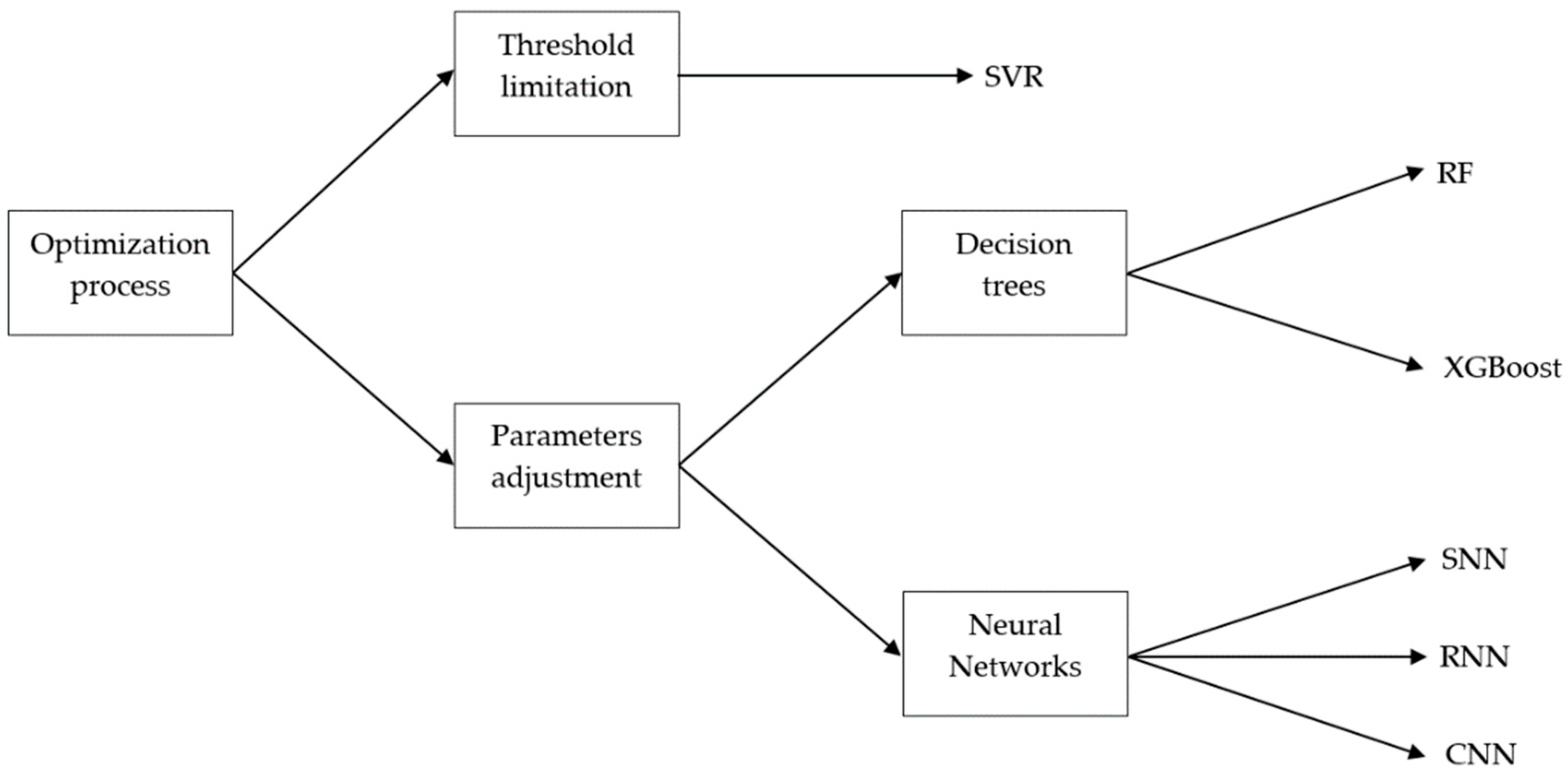
The cost function differs depending on the learning technique used. The selection of the technique is based on the way the model learns to reproduce the training data. There are two possibilities, imposing a constraint on a threshold, or through the iterative adjustment of the learning parameters through the minimization of the error between the obtained result with respect to the real values. Consisting of the first of them to the training carried out by the SVR model, and the second, to the rest of the models. Depending on the modeling options of the latter, it is possible to differentiate between decision trees techniques, represented by RF, and XGBoost, or Neural Networks, i.e., SNN, RNN, and CNN. Figure 1 presents the phase diagram for the application of the cost function according to the method to be used.

Figure 1.
Phase diagram for the application of the Artificial Intelligence methods according to the optimization process.
2.2.1. Optimization Carried out by Threshold Limitation
These type of technique maps the training data to approximate the regression line by means of a hyperplane considering a threshold, boundary lines, and is mainly represented by SVR models. In contrast to the other models, which seek to minimize the error between the forecast and the objective variable, this model seeks to contain the data in the boundary lines [49]. Thus, the cost function does not consider the loss function and is evaluated by adjusting the weights of the independent variables, , Equation (1).
where, is the number of independent variables, is a hyperparameter that represents the regularization, and , is the slack margin [50]. The representation of this model can be seen in Figure 2.
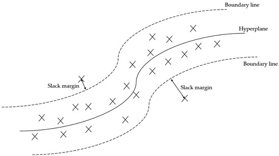
Figure 2.
Configuration of a Support Vector Regression model.
2.2.2. Optimization Carried out by Parameters Adjustment
The general purpose of this models is to have the minimum error that these have in the forecast of the objective variable. The mean squared error is selected as the loss function, , to assess the accuracy of the models, Equation (2).
where, is the number of samples, is the forecast variable at time k, and is the objective variable at time k.
- Decision trees
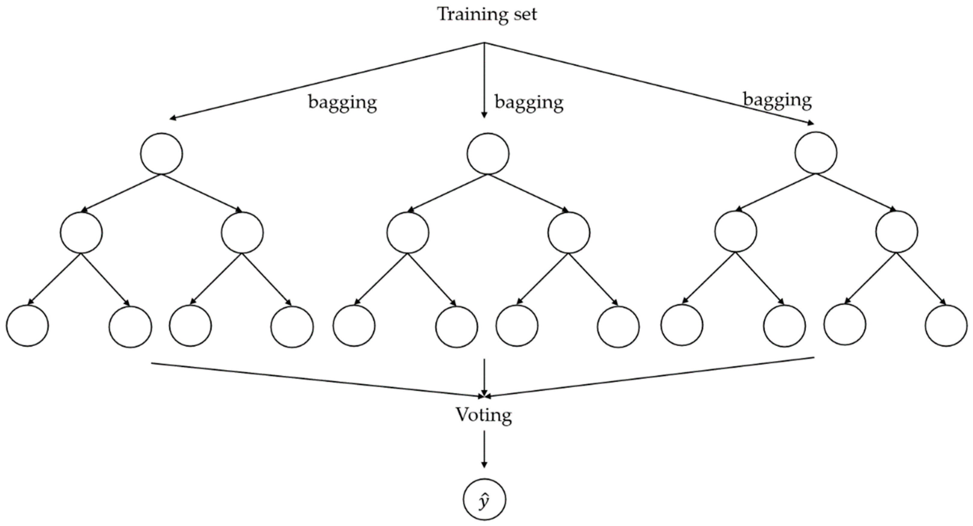
RF model consists of the synchronized operation of several unrelated decision trees. Training process is made through bagging. This technique ensures the independence of each of the decision trees and reduces the sensibility of the model to data variations [51,52]. The cost function of this model, , depends on the complexity of each of the decision trees, , in addition to the loss function, Equation (3).
where refers to the evaluated decision tree. The final result is weighted by the number of decision trees. Figure 3 shows a representative version of the random forest models.
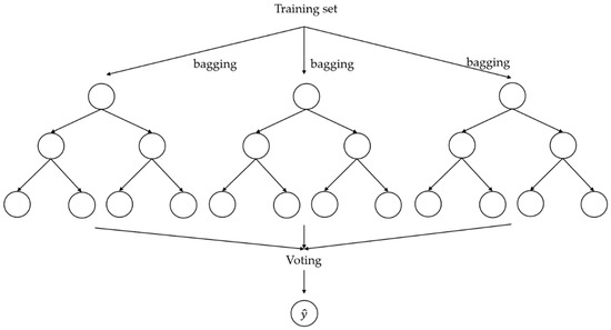
Figure 3.
Configuration of a Random Forest model.
The main problem with the RF model is that it has decision trees without a good forecast, known as weak learners [53]. XGBoost model face this issue through additive learning. With this technique, the learning process considers time steps prior to forecasting the current value. This generates a modification in the cost function, which is commonly represented as a second-order expansion of the Taylor series, Equation (4). Thus, it is possible to obtain an accurate optimization of the problem quickly [54].
where, is the considered iteration, is the definition of the -tree, is the first partial derivative of the loss function with respect to , and is the second partial derivative of the loss function with respect to Figure 3 also captures the decomposition of this model.
- Neural Networks
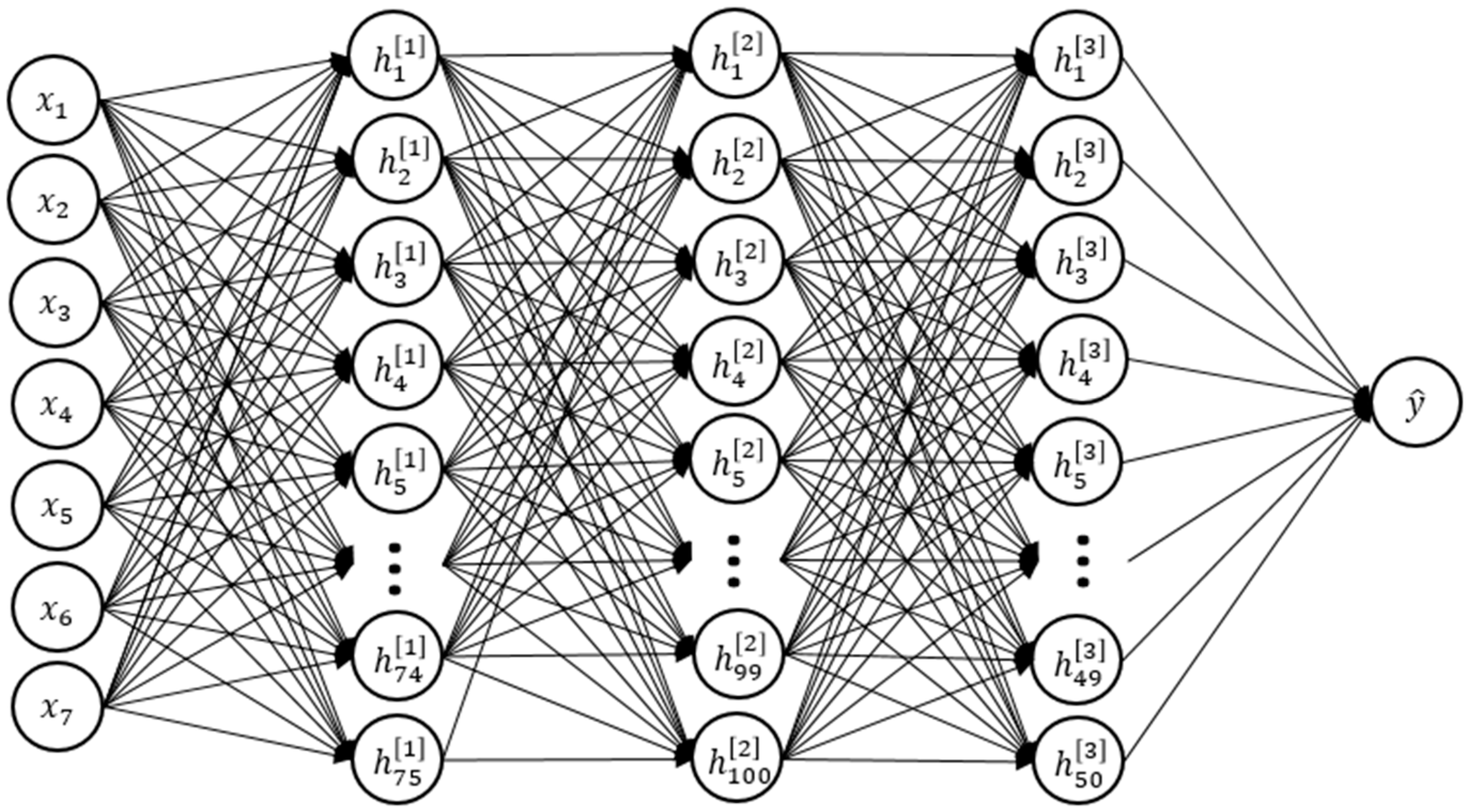
Deep Learning models have been configured using the bottleneck composition, where the number of hidden neurons decreases as the number of hidden layers increases [55]. Patterns are extracted by means of the interconnection of the different sets of neurons. The Deep Learning models propagate information from the input layer to the output layer through these hidden interconnections [56]. The cost function in these models is directly governed by the loss function, Equation (5).
The SNN model is the basic configuration. In this model, neurons in one layer are fully connected to the previous layer. This type of layer is also known as dense layer. The other configurations, i.e., RNN model and CNN model, are commonly applied together with the SNN model. Thus, both models are used as the first hidden layers to extract important information. Then, the model changes and has several dense layers, typical of SNN modeling. The typical configuration of Deep Learning models is shown in Figure 4.

Figure 4.
Configuration of a Deep Learning model.
The RNN model is a derivative of the SNN model that retains the important information from previous time steps, i.e., it has memory. LSTM (Long Short-Term Memory) is the best known type in the RNN modeling. This presents a series of internal mechanisms, gates, that regulate the flux of information that must be retained or forgotten [57,58]. Due to the memory fact, the RNN model is more complex than the SNN model as it has more parameters to train.
The CNN model is also a derivative of the SNN model. This keeps important details and avoids irrelevant information. This is due to the fact that CNN model applies convolutions to the data through a kernel. In contrast to SNN and RNN models, the kernel is common to each set of neurons [59,60]. Thus, CNN model has a lower quantity of parameters to train. The multidimensionality of the output coming from the convolution is resolved by applying a flattening layer since the SNN needs a 1D input [61].
2.3. Error Assesment
To carry out a comparative study of the performance of Artificial Intelligence models, several metrics have been computed. These have been evaluated together with its standard deviation (sd). The bias of the variable to be forecast is obtained with the normalized Mean Bias Error (nMBE), Equation (6). Positive values indicate underestimation and negative, overestimation.
where, is the maximum value of the objective variable.
The measurement of how spread out are these residuals are computed with the normalized Mean Squared Error (nRMSE). It is considered an excellent error metric for numerical predictions. This gives an indication of the model’s ability to forecast the overall load shape that is reflected in the data, Equation (7), which is strictly positive and the results decrease as the error approaches zero.
The coefficient of determination (R2) indicates how close the forecast values are to the regression line of the objective values, Equation (8). It is a common metric to evaluate numerical predictions. Its values are limited in the range [0, 1], where higher values mean that the forecast variable matches the objective variable and lower ones do not.
where, is the mean value of the objective variable.
3. Case Study
The Artificial Intelligence models described in previous section have been validated with photovoltaic production data collected from a single-family dwelling located in the state of Maryland, United States [62,63]. The photovoltaic installation faces south and has a nominal power of 10.24 kW. Nevertheless, the photovoltaic power data are collected once the inversion has been made, which has an efficiency of 93%. Thus, the maximum useful power is 9.52 kW, so this value has been selected to normalize the metrics.
The measurements correspond to hourly data divided into 2 periods of 1 year, from July 2013 to July 2014, and from February 2015 to February 2016. The composition of features selected to validate the methodology presented above are irradiance, as an independent variable, and photovoltaic production, as a dependent variable. The quality of the data is excellent, with a validity of 98.95% in irradiation, and 96.91% in photovoltaic production, once the data cleaning process has been applied.
With knowledge of the domain and through the data cleaning process with a functional approach to the data set in weekly periods, inconsistent data have been corrected, i.e., data with structural errors, and missing data has been repaired in periods where the gap consists of a maximum of 3 h. Duplicate and irrelevant data have also been removed. With data mining techniques the temporal variables: hour of the day, day of the week and day of the year have been extracted. After several runs of the analysis, mean normalization is the one that better fits the objective variable. Consequently, this type of normalization is shown in the results section. To retain the information provided by the wrong data and ensure data continuity, one hot encoding has been used. Figure 5 graphically shows the main configuration used for forecasting with the Artificial Intelligence methods.

Figure 5.
Photovoltaic production forecasting problem, where the Artificial Intelligence model corresponds to the considered Machine Learning or Deep Learning model.
Artificial Intelligence methods are carried out of the 10-fold cross-validation technique. In order to reproduce and compare the results, a seed has been applied. The data division is 95% training, where 90% corresponds to the train split and 5% to the validation split, and the remaining 5% is test. The hyperparameters used to perform the training process are 100 epochs and a batch size of 64. The optimizer used is the adaptive movement estimation algorithm, Adam, with a learning rate of 0.001.
The Deep Learning models are made using bottleneck composition. The SNN model is composed of 4 dense layers of 100, 75, 50, and 25. Its activation functions are Linear except for the last hidden layer and the output layer, whose activation functions are ReLU. Short-term memory in the RNN model is set to 6 time steps, i.e., 6 h. In this model, the first hidden layer corresponds to the LSTM with 64 neurons. The rest of the model is composed of dense layers with 40 and 20 neurons. On the one hand, the activations functions of the LSTM layer are the typical ones. On the other hand, the linear activation function is selected for the first dense layer and the rest of layers are ReLU. The convolution layer in the CNN model has 64 filters with a kernel of 3. Padding is not considered and the stride is 1. After the convolutional layer, a flattening layer is applied for the imposition of two dense layers. The number of neurons and the activations functions are the same as the considered in the RNN model.
4. Results
This section discusses the affinity of the use of the different Artificial Intelligence methods developed to forecast photovoltaic production. The characteristics of the photovoltaic system in the building studied and the general information of the generated models are detailed in the previous section. The mean errors obtained by means of the cross-validation technique in each of the splits, i.e., training, validation (dev), and testing, are shown in Table 1.

Table 1.
Average error obtained with the cross-validation method in different Artificial Intelligence methods.
Furthermore, even though RF y XGBoost models appear to generate accurate results, these are not good. It can be shown from the nRMSE metric that the forecast in validation set, also in the test set, has a large gap with respect to the training set. So, it can be concluded that the convergence of these models is not adequate since there is an overfitting in the results. Consequently, these models cannot be considered as a good model to forecast photovoltaic production.
Finally, the other three models, SVR, SNN, and CNN, generate quite good results. These fit in all sets. The CNN model stands out, which, due to the extraction of patterns from convolutions, has a regular and precise results. Thus, it can be said that this model is the best for forecasting photovoltaic production. SVR and SNN are also adjusted, but with the results of the metrics that are shown, it is not possible to conclude which is the best between the two.
Solar irradiation is zero by definition at night, so there is no photovoltaic production in this period. Therefore, it can be though that nights are an irrelevant period in the forecast of photovoltaic production. The metrics previously analyzed in Table 1 may have erroneous results since it is possible that the models are forecasting perfectly, or not, the nights. Table 2 shows the results of the models without nighttime consideration to evaluate their accuracy in the relevant periods.

Table 2.
Averaged error obtained with the cross-validation method in different Artificial Intelligence methods without night consideration.
As can be verified with Table 2, the considerations previously adopted with Table 1 can be confirmed. The RNN model is not particularly good; RF and XGBoost models are overfitting; CNN is the best model; and SNN, and SVR are good models but not as good as the CNN model. Observing Table 2, it can be concluded that SVR model is better than SNN model due to the consistency in its results. Thus, the SVR model will have better fits in irregular periods. Furthermore, the fact of considering the entire period does not significantly affect the results. All consideration can allow modeling to be more robust to possible data changes due to continuity and experience.
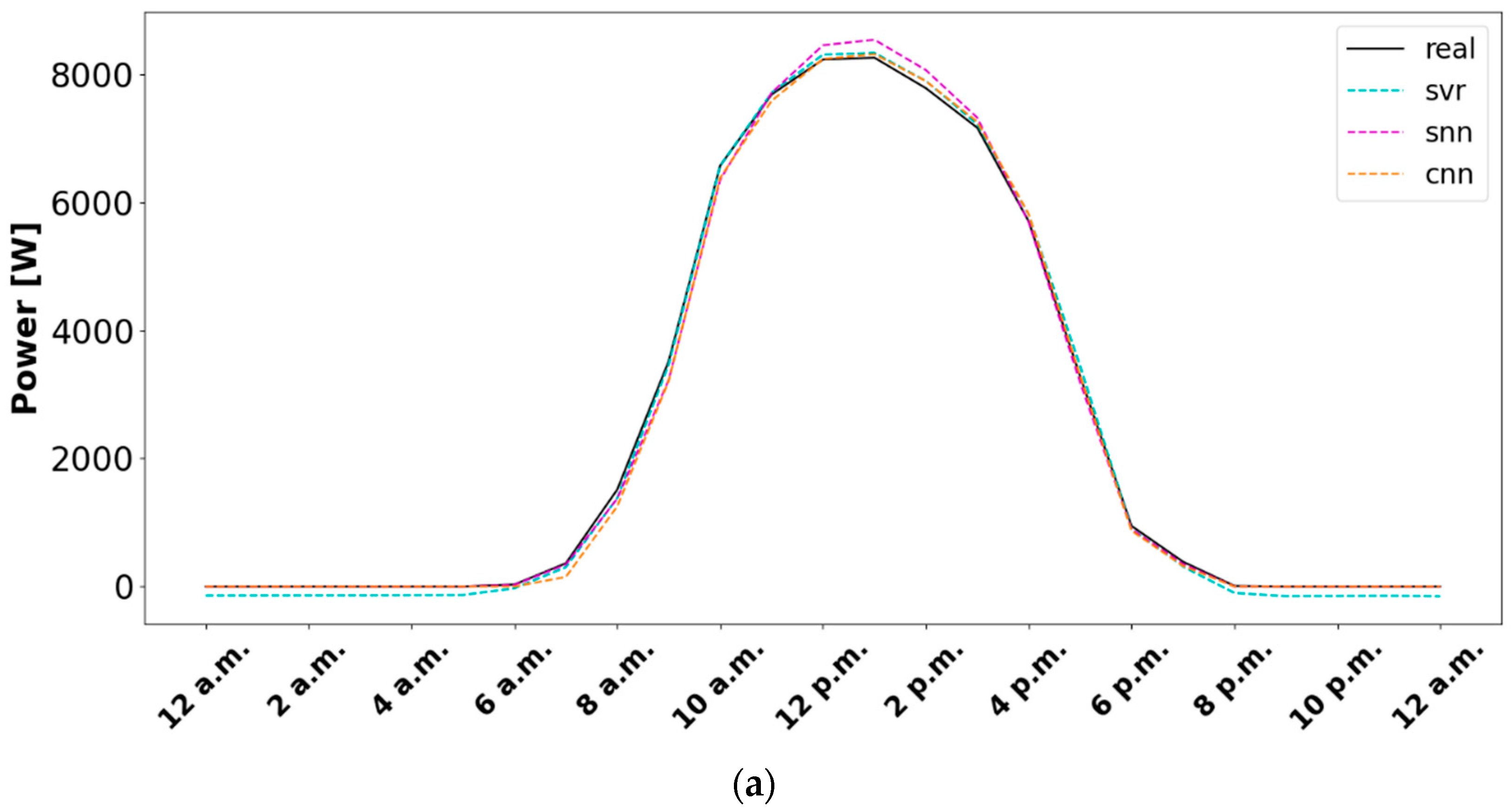
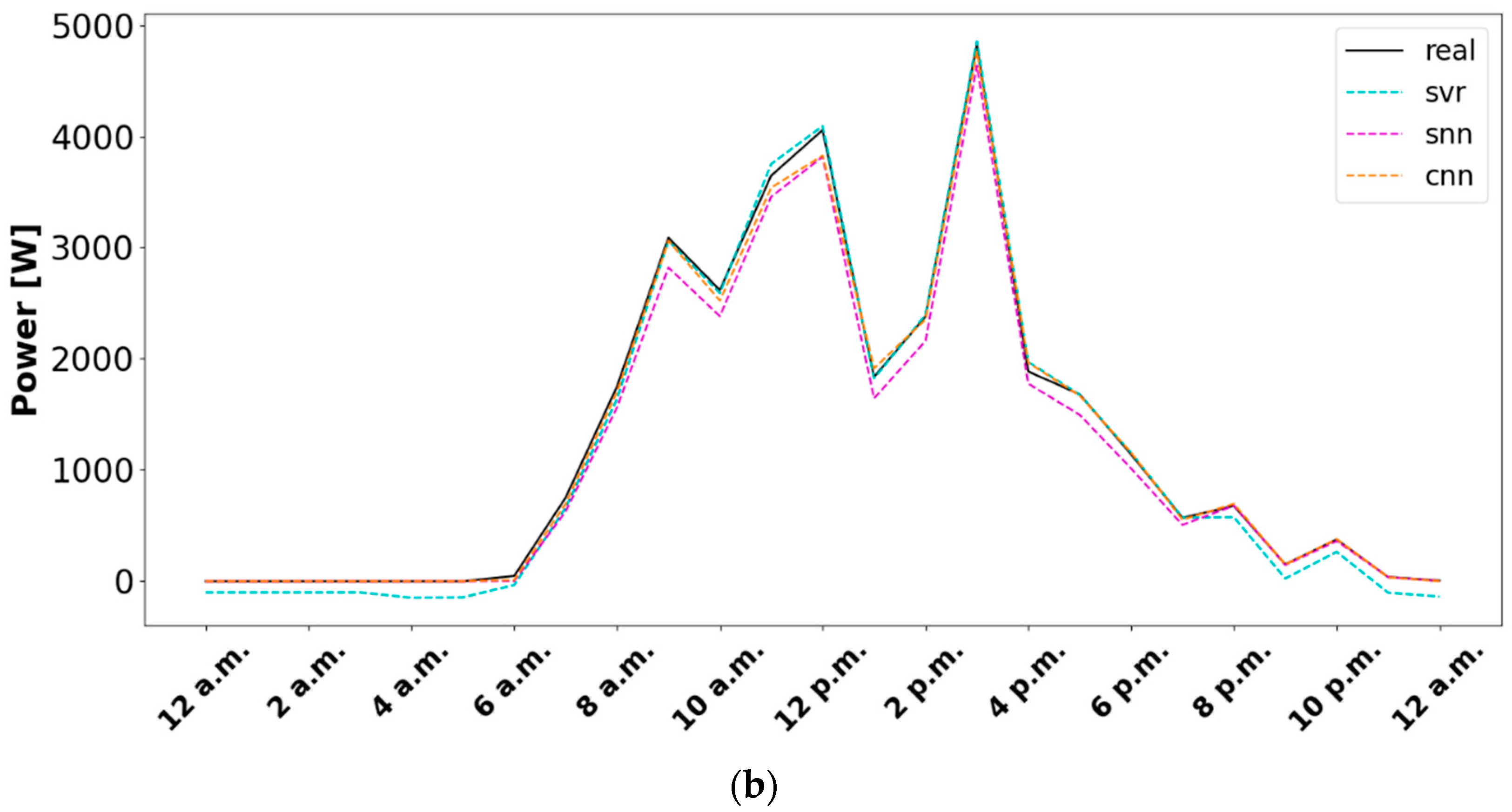
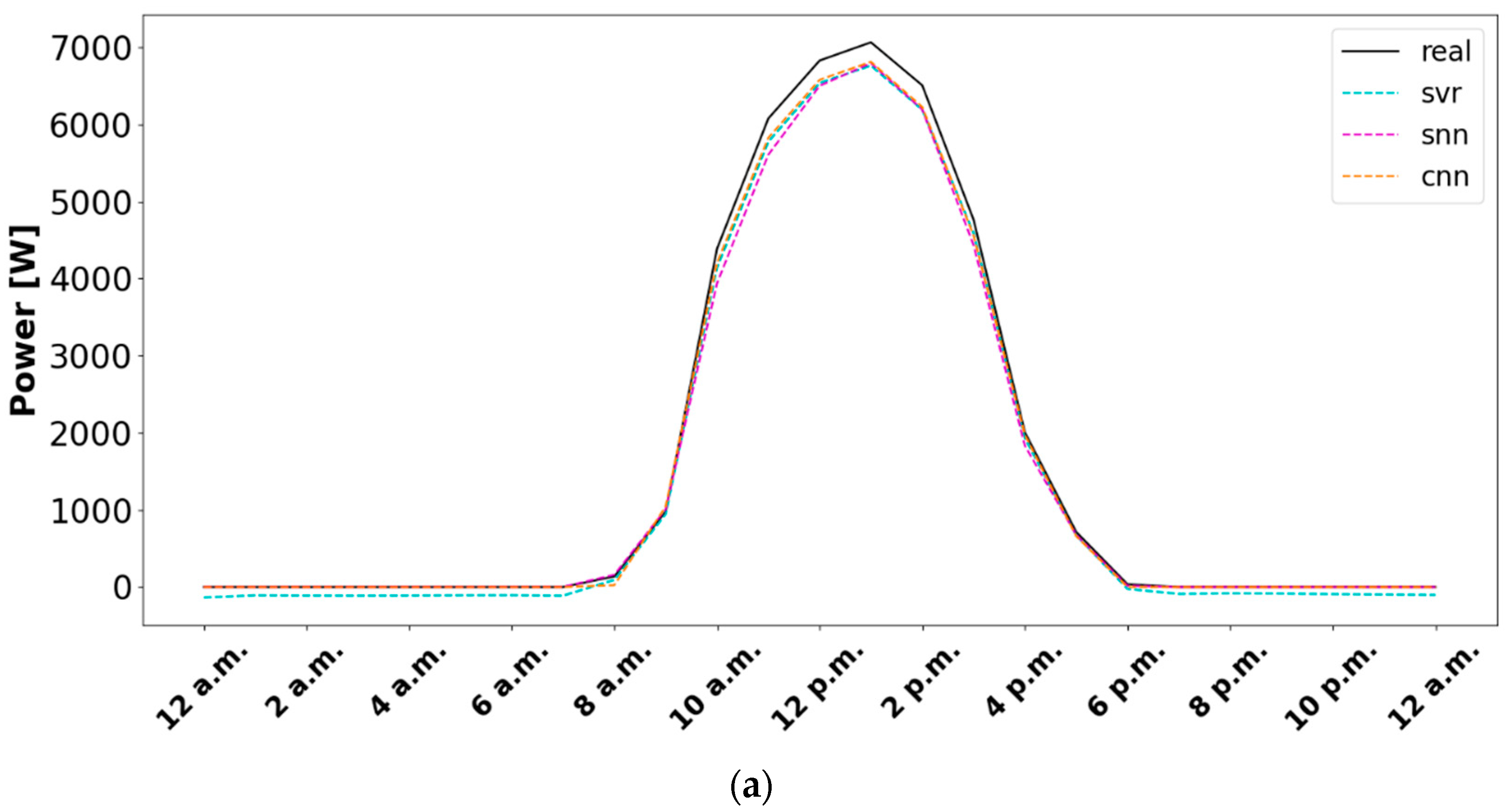
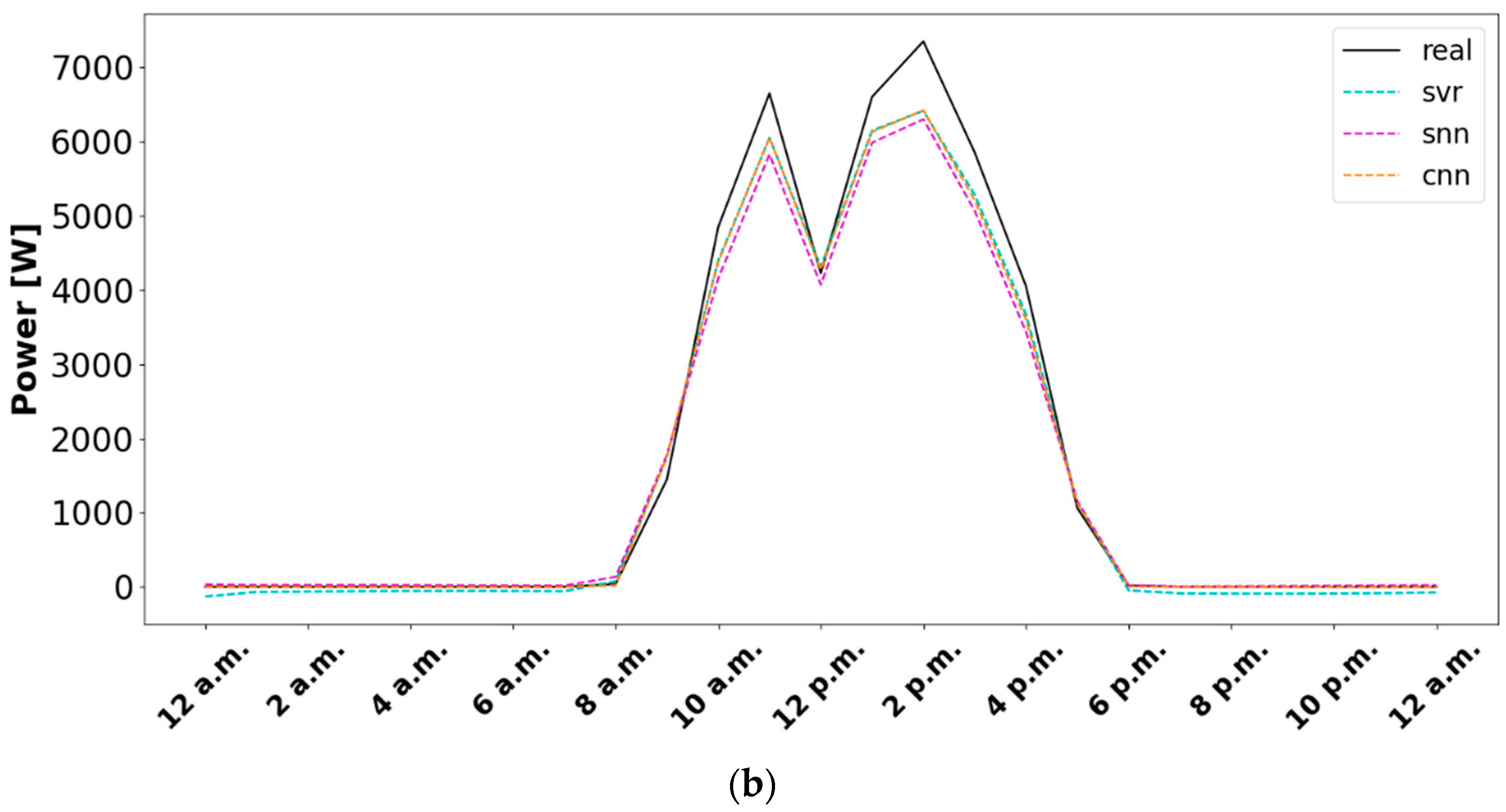
As determined, SVR, SNN, and CNN are the most appropriate models to forecast photovoltaic production. The differences between the consideration or not of the nights are not significant a priori since the models maintain the results obtained with the metrics. Then, Figure 6 graphically shows the adjustments in the train splits, and Figure 7, in test split. In both figures, the cases were selected in a couple of random periods considering the night predictions.

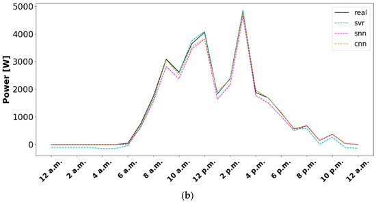
Figure 6.
Adjustments corresponding to the train split of the SVR, SNN and CNN models in the forecast of photovoltaic production: (a) Forecast on a day with good conditions, (b) Forecast on a day with variant conditions.
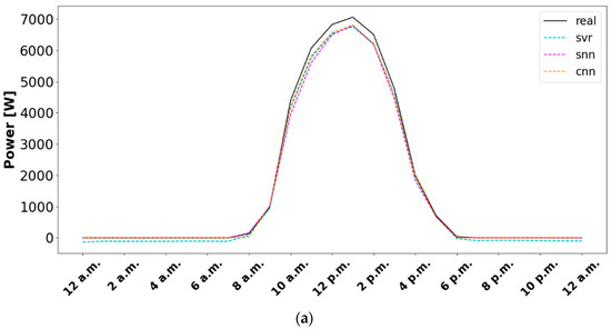
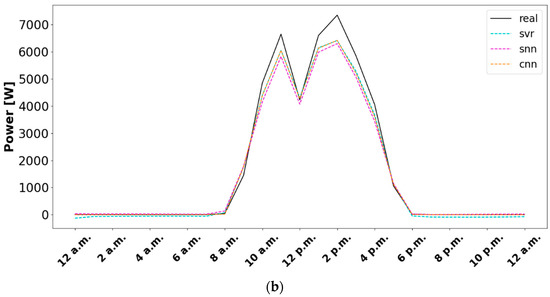
Figure 7.
Adjustments corresponding to the test split of the SVR, SNN and CNN models in the forecast of photovoltaic production: (a) Forecast on a day with good conditions, (b) Forecast on a day with variant conditions.
Figure 6 highlights the good adjustments generated by SVR, SNN, and CNN models in the training split in both conditions, smooth (a), or changing (b). As can be seen, the SVR model is the one that has periods with greater accuracy at the times that photovoltaic power occurs, i.e., during the days, as can be seen from 10 a.m. to 2 p.m. in both figures, i.e., (a) where the mean errors are −0.91% in SVR, −2.66% in SNN, and −0.75% in CNN, and (b), with mean errors of −0.26% in SVR, 2.42% in SNN, and 0.86% in CNN. However, SVR model underpredicts night periods, the error of which is around 1.50%. In contrast, the SNN and CNN models have a greater regularity in the forecast, not generating errors during nights.
As can be seen in Figure 7, the adjustments of the SVR, SNN, and CNN models are not so good in the test set, generating underpredictions. So, as can be seen in (a), from 10 a.m. to 3 p.m., where the mean errors are 3.05% in SVR, 3.49% in SNN, and 2.78% in CNN, and in (b), from 1 p.m. to 4 p.m., with mean errors of 4.08% in SVR, 5.87% in SNN, and 4.47% in CNN, neither model fits the real data perfectly. In this case, i.e., the test set, the SVR continues to underpredict the nights, where the mean error is 1.50%, meanwhile the other two models continue having no error. The SNN model has slightly worse forecasts than SVR and CNN models during nights.
5. Implication of the Study Associated with Practice and Theory
Current trends indicate that the installation of renewable power generation will have a slower increase than the energy demand in the coming years. The building sector represents a large percentage of energy consumption and, consequently, of emissions. Rooftop photovoltaic production is a commonly employed method to improve efficiency and sustainability in buildings. This technology has great potential due to the increasing improvement in its efficiency while its costs are, in comparison with others, lower. Moreover, the impact on the reduction of greenhouse gasses is enormous since it is estimated that it is possible to generate a quarter of current energy necessities.
Photovoltaic energy depends on the varying conditions of the day. Furthermore, there may be periods in which the information recorded is not correct. So, there are not always adequate data of the energy production to optimize its use in the building. In current rooftop photovoltaic systems, a large amount of unused data is recorded. The constant generation of data is very useful for Artificial Intelligence methods, which are capable of generating accurate forecasts in real time. These forecasts can also provide information on the state, enabling preventive maintenance and increasing the lifetime of the system.
Obtaining good forecasts of photovoltaic power through Artificial Intelligence techniques is key in the development of projects related to this source of renewable origin. The set of Artificial Intelligence techniques is suitable for making reliable and adjusted models. In addition, due to their characteristics, these models learn as more data is introduced, i.e., as time passes. In this way, the study of these models infers an increase in stability and a reduction in the difficulties that may arise, such as the management of photovoltaic resource in ZEB, nZEB, and MG.
6. Conclusions
The realization of this research can be the basis for guiding emission reduction regulations. Thus, this directly affects research in which rooftop photovoltaic production is often used to increase the sustainability and efficiency of energy consumption in buildings, such as ZEB, nZEB or MG. Thus, by carrying out this manuscript, different Machine Learning and Deep Learning models have been studied at the same time to detect which are the best options to predict photovoltaic power. The conclusions can be summarized in the following points:
- The most suitable models for forecast photovoltaic production are SVR, SNN, and CNN.
- The RF, XGBoost, and RNN models are not recommended to be used in the photovoltaic production forecasting
- The SNN and CNN models can fit with or without night consideration, CNN model being the best option.
- In the case of avoiding nights, SVR model is a very good option. It is also possible to use the RNN or CNN models.
Author Contributions
Conceptualization, M.C.-C. and D.V.; methodology, M.C.-C.; software, M.C.-C.; validation, D.V., P.E.-O. and E.G.-Á.; formal analysis, M.C.-C.; investigation, M.C.-C.; resources, E.G.-Á.; data curation, M.C.-C.; writing—original draft preparation, M.C.-C.; writing—review and editing, D.V.; visualization, D.V. and P.E.-O.; supervision, D.V. and P.E.-O.; project administration, E.G.-Á. and P.E.-O.; funding acquisition, E.G.-Á. and P.E.-O. All authors have read and agreed to the published version of the manuscript.
Funding
This research was funded by Universidade de Vigo grant number 00VI 131H 6410211.
Institutional Review Board Statement
Not applicable.
Informed Consent Statement
Not applicable.
Data Availability Statement
The data analyzed in this study is presented in [62,63].
Conflicts of Interest
The authors declare no conflict of interest.
References
- European Commission. Regulation 2018/84; European Union: Brussels, Belgium, 2018. [Google Scholar]
- Hussain, I.; Jalil, A.A.; Hassan, N.S.; Hamid, M.Y.S. Recent advances in catalytic systems for CO2 conversion to substitute natural gas (SNG): Perspective and challenges. J. Energy Chem. 2021, 62, 377–407. [Google Scholar] [CrossRef]
- Villanueva, D.; Cordeiro, M.; Feijoó, A.; Míguez, E.; Fernández, A. Effects of adding batteries in household installations: Savings, efficiency and emissions. Appl. Sci. 2020, 10, 5891. [Google Scholar] [CrossRef]
- International Energy Agency (IEA). Global Energy Review 2020; IEA: Paris, France, 2020. [Google Scholar]
- International Energy Agency (IEA). Electricity Market Report—July 2021; IEA: Paris, France, 2021. [Google Scholar]
- European Commission. 100 Climate-Neutral Cities by 2030—by and for the Citizens; European Union: Brussels, Belgium, 2020. [Google Scholar]
- European Commission. A European Long-Term Strategic Vision for a Prosperous, Modern, Competitive and Climate Neutral Economy; Eurpean Union: Brussels, Belgium, 2018. [Google Scholar]
- Ballesteros-Gallardo, J.A.; Arcos-Vargas, A.; Núñez, F. Optimal Design Model for a Residential PV Storage System. An Application to the Spanish Case. Sustainability 2021, 13, 575. [Google Scholar] [CrossRef]
- Solar Power Europe. EU Market Outlook for Solar Power/2019–2023; Solar Power Europe: Brussels, Belgium, 2019. [Google Scholar]
- Belussi, L.; Barozzi, B.; Bellazzi, A.; Danza, L.; Devitofrancesco, A.; Fanciulli, C.; Ghellere, M.; Guazzi, G.; Meroni, I.; Salamone, F.; et al. A review of performance of zero energy buildings and energy efficiency solutions. J. Build. Eng. 2019, 25, 100772. [Google Scholar] [CrossRef]
- Brambilla, A.; Salvalai, G.; Imperadori, M.; Sesana, M.M. Nearly zero energy building renovation: From energy efficiency to environmental efficiency, a pilot case study. Energy Build. 2018, 166, 271–283. [Google Scholar] [CrossRef]
- Zia, M.F.; Elbouchikhi, E.; Benbouzid, M. Microgrids energy management systems: A critical review on methods, solutions, and prospects. Appl. Energy 2018, 222, 1033–1055. [Google Scholar] [CrossRef]
- Villanueva, D.; Cordeiro-Costas, M.; Feijoó-Lorenzo, A.E.; Fernández-Otero, A.; Míguez-García, E. Towards DC energy efficient homes. Appl. Sci. 2021, 11, 6005. [Google Scholar] [CrossRef]
- López-Gómez, J.; Ogando-Martínez, A.; Troncoso-Pastoriza, F.; Febrero-Garrido, L.; Granada-Álvarez, E.; Orosa-García, J.A. Photovoltaic Power Prediction Using Artificial Neural Networks and Numerical Weather Data. Sustainability 2020, 12, 10295. [Google Scholar] [CrossRef]
- Zhang, Q.; Yang, L.T.; Chen, Z.; Li, P. A survey on deep learning for big data. Inf. Fusion 2018, 42, 146–157. [Google Scholar] [CrossRef]
- Oh, S. Comparison of a Response Surface Method and Artificial Neural Network in Predicting the Aerodynamic Performance of a Wind Turbine Airfoil and Its Optimization. Appl. Sci. 2020, 10, 6277. [Google Scholar] [CrossRef]
- Lei, Y.; Yang, B.; Jiang, X.; Jia, F.; Li, N.; Nandi, A.K. Applications of machine learning to machine fault diagnosis: A review and roadmap. Mech. Syst. Signal Process. 2020, 138, 106587. [Google Scholar] [CrossRef]
- Portugal, I.; Alencar, P.; Cowan, D. The use of machine learning algorithms in recommender systems: A systematic review. Expert Syst. Appl. 2018, 97, 205–227. [Google Scholar] [CrossRef]
- Lecun, Y.; Bengio, Y.; Hinton, G. Deep learning. Nature 2015, 521, 436–444. [Google Scholar] [CrossRef] [PubMed]
- Martínez-Comesaña, M.; Ogando-Martínez, A.; Troncoso-Pastoriza, F.; López-Gómez, J.; Febrero-Garrido, L.; Granada-Álvarez, E. Use of optimised MLP neural networks for spatiotemporal estimation of indoor environmental conditions of existing buildings. Build. Environ. 2021, 205, 108243. [Google Scholar] [CrossRef]
- Das, U.K.; Tey, K.S.; Seyedmahmoundian, M.; Mekhilef, S.; Idris, M.Y.I.; van Deventer, W.; Horan, B.; Stojcevski, A. Forecasting of photovoltaic power generation and model optimization: A review. Renew. Sustain. Energy Rev. 2018, 81, 912–928. [Google Scholar] [CrossRef]
- van der Meer, D.W.; Widén, J.; Munkhammar, J. Review on probabilistic forecasting of photovoltaic power production and electricity consumption. Renew. Sustain. Energy Rev. 2018, 81, 1484–1512. [Google Scholar] [CrossRef]
- Schmidhuber, J. Deep Learning in Neural Networks: An Overview. Neural Netw. 2015, 61, 85–117. [Google Scholar] [CrossRef]
- Bottou, L.; Curtis, F.E.; Nocedal, J. Optimization Methods for Large-Scale Machine Learning. SIAM Rev. 2018, 60, 223–311. [Google Scholar] [CrossRef]
- Lu, C.; Shi, J. Relative density prediction of additively manufactured Inconel 718: A study on genetic algorithm optimized neural network models. Rapid Prototyp. J. 2022, 28, 1425–1436. [Google Scholar] [CrossRef]
- Khorasani, M.; Ghasemi, A.H.; Leary, M.; Sharabian, E.; Cordova, L.; Gibson, I.; Downing, D.; Bateman, S.; Brandt, M.; Rolfe, B. The effect of absorption ratio on meltpool features in laser-based powder bed fusion of IN718. Opt. Laser Technol. 2022, 153, 108263. [Google Scholar] [CrossRef]
- Rashed, K.; Kafi, A.; Simons, R.; Bateman, S. Fused filament fabrication of nylon 6/66 copolymer: Parametric study comparing full factorial and Tauguchi design of experiments. Rapid Prototyp. J. 2022, 28, 1111–1128. [Google Scholar] [CrossRef]
- Agrawal, R. Sustainable design guidelines for additive manufacturing applications. Rapid Prototyp. J. 2022, 28, 1221–1240. [Google Scholar] [CrossRef]
- Alshehri, M.; Kumar, M.; Bhardwaj, A.; Mishra, S.; Gyani, J. Deep Learning Based Approach to Classify Saline Particles in Sea Water. Water 2021, 13, 1251. [Google Scholar] [CrossRef]
- Anjos, O.; Iglesias, C.; Peres, F.; Martínez, J.; García, A.; Taboada, J. Neural networks applied to discriminate botanical origin of honeys. Food Chem. 2015, 175, 128–136. [Google Scholar] [CrossRef]
- Marichal-Plasencia, G.N.; Camacho-Espino, J.; Ávila Prats, D.; Peñate Suárez, B. Machine Learning Models Applied to Manage the Operation of a Simple SWRO Desalination Plant and Its Application in Marine Vessels. Water 2021, 13, 2547. [Google Scholar] [CrossRef]
- Girshick, R.; Donahue, J.; Darrell, T.; Malik, J. Region-based convolutional networks for accurate object detection and segmentation. IEEE Trans. Pattern Anal. Mach. Intell. 2016, 38, 7112511. [Google Scholar] [CrossRef]
- Jun, Y.; Leyuan, F.; Min, H. Spectral-Spatial Latent Reconstruction for Open-Set Hyperspectral Image Classification. IEEE Trans. Image Process. 2022, 31, 5227–5241. [Google Scholar] [CrossRef]
- Li, D.; Dawei, L.; Qifan, T.; Jun, W. Yarn Density Measurement for 3-D Braided Composite Preforms Based on Rotation Object Detection. IEEE Trans. Instrum. Meas. 2022, 71, 5016711. [Google Scholar] [CrossRef]
- Chen, L.; Hu, X.; Xu, T.; Kuang, H.; Li, Q. Turn Signal Detection During Nighttime by CNN Detector and Perceptual Hashing Tracking. IEEE Trans. Intell. Transp. Syst. 2017, 18, 3303–3314. [Google Scholar] [CrossRef]
- Xuemin, H.; Bo, T.; Long, C.; Sheng, S.; Xiuchi, T. Learning a Deep Cascaded Neural Network for Multiple Motion Commands Prediction in Autonomous Driving. IEEE Trans. Intell. Transp. Syst. 2021, 22, 7585–7596. [Google Scholar] [CrossRef]
- Hui, Z.; Liuchen, W.; Yurong, C.; Ruibo, C.; Senlin, K.; Yaonan, W.; Jianwen, H.; Jonathan, W. Attention-Guided Multitask Convolutional Neural Network for Power Line Parts Detection. IEEE Trans. Instrum. Meas. 2022, 71, 5008213. [Google Scholar] [CrossRef]
- Shi, J.; Lee, W.-J.; Liu, Y.; Yang, Y.; Wang, P. Forecasting Power Output of Photovoltaic Systems Based on Weather Classification and Support Vector Machines. IEEE Trans. Ind. Appl. 2012, 48, 1064–1069. [Google Scholar] [CrossRef]
- De Paiva, G.M.; Pimentel, S.P.; Alvarenga, B.P.; Marra, E.G.; Mussetta, M.; Leva, S. Multiple Site Intraday Solar Irradiance Forecasting by Machine Learning Algorithms: MGGP and MLP Neural Networks. Energies 2020, 13, 3005. [Google Scholar] [CrossRef]
- Mehrkanoon, S. Deep shared representation learning for weather elements forecasting. Knowl. Based Syst. 2019, 179, 120–128. [Google Scholar] [CrossRef]
- Abedinia, O.; Lotfi, M.; Bagheri, M.; Sobhani, B.; Shafie-Khah, M.; Catalao, J.P.S. Improved EMD-Based Complex Prediction Model for Wind Power Forecasting. IEEE Trans. Sustain. Energy 2020, 11, 2790–2802. [Google Scholar] [CrossRef]
- Ridzuan, F.; Zainon, W.M.N.W. A Review on Data Cleansing Methods for Big Data. Procedia Comput. Sci. 2019, 161, 731–738. [Google Scholar] [CrossRef]
- Munappy, A.R.; Bosch, J.; Olsson, H.H.; Arpteg, A.; Brinne, B. Data management for production quality deep learning models: Challenges and solutions. J. Syst. Softw. 2022, 191, 111359. [Google Scholar] [CrossRef]
- Singh, D.; Singh, B. Investigating the impact of data normalization on classification performance. Appl. Soft Comput. 2020, 97, 105524. [Google Scholar] [CrossRef]
- Saleh, R.; Fleyeh, H. Using Supervised Machine Learning to Predict the Status of Road Signs. Transp. Res. Procedia 2022, 62, 221–228. [Google Scholar] [CrossRef]
- Heaton, J. An empirical analysis of feature engineering for predictive modeling. In Proceedings of the IEEE SOUTHEASTCON, Norfolk, VA, USA, 30 March–3 April 2016; pp. 1–6. [Google Scholar] [CrossRef] [Green Version]
- Verdonck, T.; Baesens, B.; Óskarsdóttir, M.; vanden Broucke, S. Special issue on feature engineering editorial. Mach. Learn. 2021, 1–12. [Google Scholar] [CrossRef]
- Feng, Y.; Tu, Y. Phases of learning dynamics in artificial neural networks: In the absence or presence of mislabeled data. Mach. Learn. Sci. Technol. 2021, 2, 043001. [Google Scholar] [CrossRef]
- Vrablecová, P.; Ezzeddine, A.B.; Rozinajová, V.; Šárik, S.; Sangaiah, A.K. Smart grid load forecasting using online support vector regression. Comput. Electr. Eng. 2018, 65, 102–117. [Google Scholar] [CrossRef]
- Zhong, H.; Wang, J.; Jia, H.; Mu, Y.; Lv, S. Vector field-based support vector regression for building energy consumption prediction. Appl. Energy 2019, 242, 403–414. [Google Scholar] [CrossRef]
- Voyant, C.; Notton, G.; Kalogirou, S.; Nivet, M.-L.; Paoli, C.; Motte, F.; Fouilloy, A. Machine Learning methods for solar radiation forecasting: A review. Renew. Energy 2017, 105, 569–582. [Google Scholar] [CrossRef]
- Booth, A.; Gerding, E.; McGroarty, F. Automated trading with performance weighted random forests and seasonality. Expert Syst. Appl. 2014, 41, 3651–3661. [Google Scholar] [CrossRef]
- Touzani, S.; Granderson, J.; Fernandes, S. Gradient boosting machine for modeling the energy consumption of commercial buildings. Energy Build. 2018, 158, 1533–1543. [Google Scholar] [CrossRef]
- Martínez-Comesaña, M.; Febrero-Garrido, M.; Granada-Álvarez, E.; Martínez-Torres, J.; Martínez-Mariño, S. Heat Loss Coefficient Estimation Applied to Existing Buildings through Machine Learning Models. Appl. Sci. 2020, 10, 8968. [Google Scholar] [CrossRef]
- Ren, S.; He, K.; Girshick, R.; Sun, J. Faster R-CNN: Towards Real-Time Object Detection with Region Proposal Networks. IEEE Trans. Pattern Anal. Mach. Intell. 2017, 39, 1137–1149. [Google Scholar] [CrossRef]
- Chang, G.W.; Lu, H.J.; Chang, Y.R.; Lee, Y.D. An improved neural network-based approach for short-term wind speed and power forecast. Renew. Energy 2017, 105, 301–311. [Google Scholar] [CrossRef]
- Kong, W.; Dong, Z.Y.; Jia, Y.; Hill, D.J.; Xu, Y.; Zhang, Y. Short-Term Residential Load Forecasting Based on LSTM Recurrent Neural Network. IEEE Trans. Smart Grid 2017, 10, 841–851. [Google Scholar] [CrossRef]
- Zhao, H.; Sun, S.; Jin, B. Sequential Fault Diagnosis Based on LSTM Neural Network. IEEE Access 2018, 6, 12929–12939. [Google Scholar] [CrossRef]
- Ju, Y.; Sun, G.; Chen, Q.; Zhang, M.; Zhu, H.; Rehman, M.U. A Model Combining Convolutional Neural Network and LightGBM Algorithm for Ultra-Short-Term Wind Power Forecasting. IEEE Access 2019, 7, 28309–28318. [Google Scholar] [CrossRef]
- Pereira, S.; Pinto, A.; Alves, V.; Silva, C.A. Brain Tumor Segmentation Using Convolutional Neural Networks in MRI Images. IEEE Trans. Med. Imaging 2016, 35, 1240–1251. [Google Scholar] [CrossRef] [PubMed]
- Zhang, J.; Lu, C.; Li, X.; Kim, H.J.; Wang, J. A full convolutional network based on DenseNet for remote sensing scene classification. Math. Biosci. Eng. 2019, 16, 3345–3367. [Google Scholar] [CrossRef]
- William, H.; Fanney, A.H.; Dougherty, B.; Payne, W.V.; Ullah, T.; Ng, L.; Omar, F. Net Zero Energy Residential Test Facility Instrumented Data; Year 2; National Institute of Standards and Technology: Gaithersburg, MD, USA, 2016. [CrossRef]
- William, H.; Chen, T.H.; Dougherty, B.; Fanney, A.H.; Ullah, T.; Payne, W.V.; Ng, L.; Omar, F. Net Zero Energy Residential Test Facility Instrumented Data; Year 1; National Institute of Standards and Technology: Gaithersburg, MD, USA, 2018. [CrossRef]
Publisher’s Note: MDPI stays neutral with regard to jurisdictional claims in published maps and institutional affiliations. |
© 2022 by the authors. Licensee MDPI, Basel, Switzerland. This article is an open access article distributed under the terms and conditions of the Creative Commons Attribution (CC BY) license (https://creativecommons.org/licenses/by/4.0/).

