Article

Physics-Informed Data-Driven Model for Predicting Streamflow: A Case Study of the Voshmgir Basin, Iran

1
Department of Smart Cities, Chung-Ang University, Seoul 06974, Korea
2
Department of Civil Engineering, New Mexico State University, Las Cruces, NM 88003, USA
3
School of Engineering, University of Guelph, Guelph, ON N1G 2W1, Canada
4
Bedford Institute of Oceanography, Dartmouth, NS B2Y 4A2, Canada
5
Department of Civil and Environmental Engineering, Chung-Ang University, Seoul 06974, Korea
6
Department of Civil and Environmental Engineering and Water Resources Research Center, University of Hawaii at Manoa, Honolulu, HI 96822, USA
*
Author to whom correspondence should be addressed.
Appl. Sci. 2022, 12(15), 7464; https://doi.org/10.3390/app12157464
Submission received: 8 June 2022 / Revised: 1 July 2022 / Accepted: 17 July 2022 / Published: 25 July 2022
(This article belongs to the Section Earth Sciences)

Abstract

:
Accurate rainfall-runoff modeling is crucial for water resource management. However, the available models require more field-measured data to produce accurate results, which has been a long-term issue in hydrological modeling. Machine learning (ML) models have shown superiority in the hydrological field over statistical models. The primary aim of the present study was to advance a new coupled model combining model-driven models and ML models for accurate rainfall-runoff simulation in the Voshmgir basin in northern Iran. Rainfall-runoff data from 2002 to 2007 were collected from the tropical rainfall measuring mission (TRMM) satellite and the Iran water resources management company. The findings revealed that the model-driven model could not fully describe river runoff patterns during the investigated time period. The extreme learning machine and support vector regression models showed similar performances for 1-day-ahead rainfall–runoff forecasting, while the long short-term memory (LSTM) model outperformed these two models. Our results demonstrated that the coupled physically based model and LSTM model outperformed other models, particularly for 1-day-ahead forecasting. The present methodology could be potentially applied in the same hydrological properties catchment.

1. Introduction

The simulation of rainfall-runoff is a crucial task for flood control and water management, particularly for continuous flood forecasting [1]. Several studies have conducted daily discharge simulations using model-driven and data-driven models [2]. Model-driven methods usually include conceptual and physically-based models, which are also known as process-driven models [3]. Model-driven methods are rather complicated because they are based on formulas and several physical parameters [4]. In comparison, data-driven models use non-linear relations of meteorological and discharge data, which means that these models do not have sufficient knowledge about the behavior of physical parameters [5].
Model-driven models are usually knowledge-based; thus, they give significant insights into hydrological approaches. These models are divided into two types: (1) models that simulate discharge directly, such as the hydrologic modeling system (HEC-HMS) model, and (2) models that have river runoff as one of the outputs, such as the soil and water assessment tool (SWAT). The HEC-HMS model is widely used for rainfall-runoff simulation, and several studies have shown that its accuracy is acceptable for river runoff simulations [6,7,8,9]. The HEC-HMS model is applicable for simulating both event-based and continuous-based river runoff through different methods, such as the soil conservation service-curve number (SCS-CN) and deficit and constant-Snyder hydrographs for event-based and continuous-based runoff, respectively. Therefore, simulating river runoff using the HEC-HMS model depends on several input parameters. Data-driven models have conceptual differences in the modeling process [10]. The essence of data-driven models is that they use historical meteorological data to simulate and/or predict river runoff patterns. This aspect makes data-driven models more practical than model-driven models in terms of complexity because they do not require knowledge of hydrological processes. Simulating the river runoff pattern from historical hydrological time series, such as temperature and precipitation, is possible using machine learning (ML) models, viz., the artificial neural network-back propagation (ANN-BP), extreme learning machine (ELM), and support vector regression (SVR) models [11]. Kim and Kim [12] compared the SWAT and long short-term memory (LSTM) models for simulating river runoff, and found that the LSTM model outperformed the SWAT model. Several studies have compared ML models with the HEC-HMS model during typhoon events and have confirmed the superiority of ML models over the HEC-HMS model [13,14,15].
Coupled models are manipulated models that use the output of model-driven models as the input of ML models to boost the ML predictor set [16]. Anctil and Tape [17] presented a 1-day-ahead river runoff forecasting neuro-wavelet hybrid system at two sites. Other researchers have taken inspiration from their study and recently conducted studies using similar approaches. For example, Kumanlioglu and Fistikoglu [18] used daily rainfall and mean temperature data to simulate daily runoff with the génie rural à 4 paramètres journalier (GR4J) model and integrated a coupled model by using the calculated time series as the input of the ANN model to the basin in western Turkey. Their results revealed that the coupled model performed better than the GR4J and single ANN models. Farfán, et al. [19] applied a coupled model comprising two model-driven models, the rural genius model and the water evaluation and planning model (GR2M and WEAP), and an ANN model to simulate flow using meteorological data as input variables. They showed that the coupled model could compute better time series than single models. Isik, et al. [20] applied an ANN model combined with a soil conservation service (SCS) curve number (CN) to investigate the effects of land use and/or land cover on daily runoff. Their model produces highly accurate estimations. Kurian, et al. [21] suggested a coupled model that combines the HEC-HMS model with the ANN model. They forecasted a fifteen-minutes event and continuous runoff simulation, and the results indicated that the coupled model outperformed the single model. In addition, some studies have shown the importance of selecting input data for data-driven models based on methods such as the Boruta algorithm and/or cross-correlation analyses and support vector machine recursive feature elimination (SVM-RFE). They found that the selected variables could improve the results of the data-driven models [11,22].
To the best of our knowledge, several researchers have prioritized combining model-driven models and data-driven models. However, few of them applied combined model-driven models with ELM, SVR, and particularly LSTM for forecasting daily river runoff to present the best ML model. In the present study, our objectives were (i) to compare the potential of ML models with a hydrological model for simulating river runoff on a daily scale, (ii) to investigate the accuracy of the results if tropical rainfall measuring mission (TRMM) satellite data are applied in ungagged regions, and (iii) to predict 1-day-ahead river runoff with data-driven models and combine data-driven models with a hydrological model. The assumption of this study was that TRMM provides reliable satellite data for use in ungauged areas. Therefore, daily TRMM satellite data were used as inputs for the models instead of gauge precipitation data. Daily data were used because most of the studies were conducted for events and used hourly data. To the best of our knowledge, the proposed model, which is a combination of the LSTM model and HEC-HMS model and uses the SVM-RFE method to select input data, is a new model for simulating and predicting daily river runoff in the Voshmgir basin. Figure 1 shows the Voshmgir basin, which is located in the north of Iran.

2. Materials and Methods

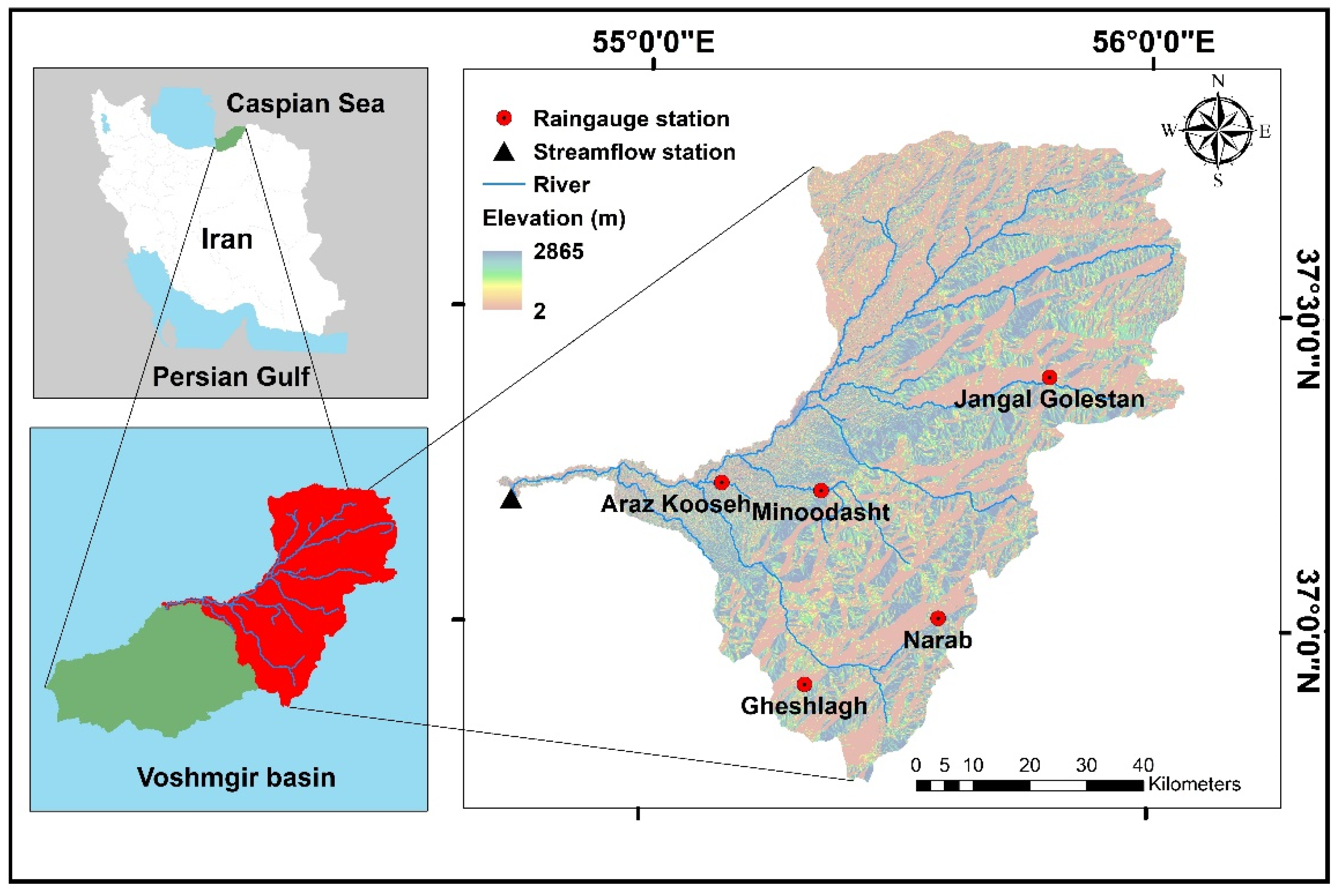
2.1. Study Area and Data Description

The Voshmgir basin is located between 54°40′ and 56°00′ E longitude and 36°50′ and 37°50′ N latitude in the east-south of the Caspian Sea. It has an area of 5748 km2, an elevation ranging from 2 to 2865 m, and an average slope of 2.2%. The basin is one of the main sources of irrigation water that is supplied to 25,000 hectares of farmland in Golestan province, Iran. The basin has a semi-arid climate, and the main river profile with a length of approximately 59 km is steep, which exposes it to soil erosion and flooding. Precipitation in this basin shows extreme nonstationary changes [23]. The annual mean precipitation is 540 mm, and 60% of the total precipitation occurs from January to June. The annual mean temperature is approximately 18 °C [24,25]. Five rainfall stations and one runoff gauging station at the outlet of the basin were considered in this study. The location, elevation, rainfall, and runoff at the gauging stations are shown in Figure 1. The daily measured river runoff data ranged from 0 to 310 m3/s. Daily measured mean temperature data and daily tropical rainfall measuring mission satellite (TRMM_3B42_daily_v7) precipitation data were collected from 2002 to 2007 from the Iran water resources management company (IWRMC) and the GES-DISC interactive online visualization and infrastructure (GIOVANNI) websites (https://giovanni.gsfc.nasa.gov/, accessed on 31 December 2019), respectively (Figure 2).

2.2. Methodology

2.2.1. Physics-Informed Data-Driven Models

Three ML models and three coupled models including the ELM, SVR, LSTM, HEC-HMS-ELM, HEC-HMS-SVR, and HEC-HMS-LSTM models were used to investigate the ability of ML and coupled methods to simulate and forecast river runoff, respectively. Huang [26] suggested that the ELM technique is more efficient than an ANN model. He found that the ELM technique has some advantages owing to its internal capabilities. There was no requirement for weight adjustment through a feasible generalization ability or a high learning speed. Various studies have revealed that the ELM is superior to an ANN [10,27,28]. Şahin, et al. [29] found that the ELM model performed 26 times better than the ANN model during the prediction of solar radiation in Turkey. Similarly, Deo and Şahin [30] applied ELM and ANN models to generate a monthly efficient drought index, and found that the prediction accuracy of the ELM model was significantly higher than that of the ANN model. In agreement with previous studies, Yaseen, et al. [31] found that the ELM’s prediction ability was superior to that of an ANN during streamflow forecasting.
The ELM model is generally an extended version of a single-hidden layer feed-forward neural network (SLFN) [32]. The structure of the model is the same as that of the standard ANN model with three layers: a single input layer, a hidden layer, and an output layer. The hidden biases and weights are chosen randomly by the Moore–Penrose generalized inverse of the hidden output matrix method instead of the fine-tuning method applied in the ANN. Because of this modification, the ELM model is capable of progressing faster than the ANN model while maintaining a sufficient generalization ability. More information on this model can be found in Huang, et al. [33]. In the current study, the ELM model was constructed through Python software using the “HP-ELM” package [34].
The support vector regression (SVR) model is an ML model used for classification and regression [35]. It uses structural risk reduction (SRR) rather than empirical risk reduction through self-learning models such as ANNs, as mentioned by Lin, et al. [36]. SVRs, which are data-driven, have recently emerged as an alternative to ANNs for hydrological studies [37]. Vapnik [38] introduced the use of SVR models from support vector machines (SVMs), which are used to solve classification problems. The SVR model has a unique architecture whose main parameters include a kernel, a hyperplane, and boundary lines. The kernel function is the key to determining the right hyperplane, which is used as a baseline to calculate the data distribution trend. SVRs have two boundary lines used to bind the positive and negative distributions. The abovementioned optimal structure and working frameworks lead to greater efficiency by avoiding overfitting. Such characteristics make SVR a popular data-driven model in the rainfall-runoff modeling field [39].
The SVR method reduces the empirical risk of reaching an adequate generalization performance by reducing the generalization error instead of the training error [40]. As mentioned earlier, the SVR model maps data into a higher-dimensional feature space to perform efficient predictions. Kernel functions are essentially tunable hyperparameters for optimal outputs. Several kernels, such as polynomial, linear, sigmoid, and radial basis functions (RBF) have been applied in various studies. However, the RBF was found to be the best among them for predicting nonlinear hydrological problems [41]. In addition, the RBF kernel outperformed the other kernels in the rainfall-runoff simulation [42]. Decreasing the calculation time with improved generalization capacity is a significant benefit of the RBF kernel [43]. Therefore, the RBF kernel was used in this study.
The long short-term memory (LSTM) model is an advanced technological neural network that has been selected as an effective model for time-series simulation and/or prediction [44]. LSTM is a type of recurrent neural network (RNN) that addresses the drawbacks of the RNN vanishing gradient by adding additional interactions [45]. The LSTM model has been applied in various areas, including rainfall-runoff simulation, handwriting identification, speed identification, and road traffic forecasting, because of its nonlinear predictive capability, faster convergence, efficient learning trends, and ability to capture the long-term correlation of the sequential series [46].
The LSTM model comprises a forget gate, an input gate, an output gate, and a cell state, as shown in Figure 3. In general, LSTM utilizes the previous state information to perform further operations. The forget gate determines the value that should be maintained or discarded. Values from the previous hidden state (ht-1) and current input (xt) move through the activation function and are computed from 0 to 1. If the computed value is close to zero, the gate forgets it, and if the value is close to 1, the gate retains it. An input gate is used to modify the state of the cell. First, we used a sigmoid function to combine the prior concealed state and the current input. The phrase “long-term memory” is frequently used to refer to the cell state. A forget gate was used to modify the cell state, whereas an input modulation gate was used to regulate the cell state. Finally, the output gate determines the next hidden state. The hidden state includes the values of previous inputs and is also used for prediction. The hidden state was represented by the output. The new cell state, as well as the new hidden state, is then transferred to the next time step in the process [47].

2.2.2. Hydrological Modeling

The hydrological model (HEC-HMS) has been extensively used to simulate rainfall-runoff processes [48]. In this model, adequate precipitation in a basin is defined by the characteristics of previously connected surfaces. The flow from the surface and channels consists of a form of direct runoff in the stream. The deficit and constant loss method based on the Snyder unit hydrograph as a transfer method suggests better estimations of the combination of soil moisture accounting (SMA) and deficit and constant based on the Clark and Snyder unit hydrograph (UH) [49]. Figure 4 shows the steps involved in this study. The streamflow hydrograph ( Q ) is derived by the interaction of the precipitation gradually increasing ( P ) with the unit hydrograph required ( U ) as follows:
Q n = m = 1 n M P m U n m + 1
where m varies between 1 and n.
The transformation of additional precipitation into direct runoff can be obtained using the Snyder unit hydrograph method. For the standard case, the Snyder formula for the peak flow can be expressed as follows:
Q P = 2.75   ·   C P   ·   A T r 5.5 ,
where T r 5.5 is basin lag, Q P is the unit hydrograph peak flow of the standard UH corresponding to 1 cm of effective rainfall ( m 3 · s 1 ), A is the catchment area (km2), and C P is the empirical coefficient relating the triangular time base to lag.
The catchment lag (hour) can be calculated as follows:
T p = C C t ( L L c ) 0.3
where C is a conversion constant 0.75 (ISI), C t is a coefficient derived from gauged watersheds, L is the length of the stream from the outlet to the upstream divide, and L c is the length along the mainstream from the outlet to the point nearest to the watershed centroid.
The HEC-HMS model can generate a simulation for forecasting river runoff from historical precipitation data, which can be obtained from different methods, including field measurements, numerical weather predictions, and satellite images. To achieve a reasonable prediction performance, the parameters in (1), (2), and (3) need to be tuned accurately according to the watershed characteristics and the input data in the calibration phase. In this study, the standard lag and the peaking coefficient ranged from 2.98 to 23.66 and 0.5 to 0.75, respectively.

2.3. Model Development and Input

This study investigated the simulation and forecasting of river runoff at a daily scale in a selected basin. To simulate the runoff, a hydrological model and three ML models were applied. The input data for the hydrological model were the TRMM precipitation data. The parameters for the HEC-HMS model were selected by trial and error in the calibration phase for the deficit and constant loss methods based on the Snyder unit hydrograph as a transfer method. Table 1 lists the parameter values for the best evaluation indices. Three ML models, the ELM, SVR, and LSTM models, were used to simulate the streamflow at daily scales in the selected basin. To achieve higher accuracy in the ML model simulation, the antecedent values of T R M M and T m e a n were used as input variables. Therefore, in addition to the input variables, a 1-day lag to a 20-day lag was applied for all input variables. The best combination of variables was chosen using the SVM-RFE approach. From Equation (4), nineteen variables were selected for the input structure in the Voshmgir basin.
Q t = f ( T m e a n ,   T R M M t 1 ,   T R M M t 3 , T R M M t 5 ,     T R M M t 11 ,   T R M M t 12 ,   T R M M t 18 ,   T R M M t 20 ,   T m e a n t 1 ,   T m e a n t 2 , T m e a n t 3 ,   T m e a n t 4 ,   T m e a n t 5 ,   T m e a n t 6   T m e a n t 7 ,   T m e a n t 8 , T m e a n t 11 ,   T m e a n t 12 ,   T m e a n t 15 )
To forecast the river runoff, three ML models and their coupled models with the HEC-HMS model were used. In the current study, T R M M precipitation at days t and t 1 and observed discharge at t and t 1 were applied as input variables of the ML models to calculate the river runoff on day t + 1 . Moreover, the simulated runoff values of the HEC-HMS model from the simulation were used as additional input variables for the three coupled models: HEC-HMS-ELM, HEC-HMS-SVR, and HEC-HMS-LSTM. Equation (5) shows the selected input variables for the coupled models.
Q t + 1 = f ( T R M M t ,   T R M M t 1 ,   Q t , Q t 1 ,   Q H E C H M S t + 1 )
The runoff data was the target variable. Data from January 2002 to December 2004 were applied to calibrate the models, and data from January 2005 to October 2007 were applied to test the models. Sola and Sevilla [50] recommended normalization of input data for the artificial neural network-back propagation (ANN-BP). They found that normalization of the input data was important to achieve better results and accelerate the calculation. Therefore, the normalization described by Equation (6) was applied to all input data of the ML models and coupled models.
n o r m a l i z e d   x = x μ σ ,
where x is the input variable, μ is the mean variable, and σ is standard deviation.

2.4. Model Parameterization

The current study applied a 10-fold cross validation method with the aim of minimizing the root mean square error (RMSE) function to set the optimal parameters of the ELM, SVR, and LSTM models for the training phase. The optimal hyperparameters were used in river runoff prediction for the validation phase, and Python was used to write the codes.
Huang, Zhu and Siew [32] recommended the ELM model owing to its small training error and norm of output weights compared with single-hidden-layer feedforward networks (SLFNs). In the ELM model, the number of neurons in hidden layer was randomly selected from 2 to 100 to achieve a model with the highest possible accuracy. A three-layer ELM model with a sigmoid activation function for the hidden layer was established. Optimal parameters were determined through a 10-fold cross-validation method with the aim of minimizing the root mean square error (RMSE) function for the training phase.
In the SVR model, the main parameters of the RBF kernel function, including the structural parameter (γ), penalty coefficient (C), and tolerance threshold (ε-precision), were optimized. For this purpose, 30 γ values from 0.0001 to 10,000, 30 C values from 0.0001 to 10,000, and 20 ε-precision values from 0.001 to 1 were chosen and evaluated. Similar to the ELM model, a 10-fold cross-validation approach was applied to find the optimized parameters.
In the LSTM model, the Keras framework with the TensorFlow back-end was used. The hyperparameters of the LSTM model include neurons, dropouts, learning rates, epoch ranges, and batch ranges. Random generation was used to tune the LSTM model. For this purpose, different neurons (10 values between 10 and 500), dropouts (10 values between 0 and 1), learning rates (10 values between 0.00001 and 0.01), epoch ranges (10 values between 10 and 1000), and batch ranges (10 values between 10 and 1000) were evaluated. Similar to the ELM and SVR models, a 10-fold cross-validation approach was applied to determine the optimized parameters of the LSTM model.
The selected parameters calculated for all three ML models consisting of the ELM, SVR, and LSTM models were applied to three coupled models: HEC-HMS-ELM, HEC-HMS-SVR, and HEC-HMS-LSTM. The optimal parameters for each ML model are presented in Table 2.

2.5. Model Evaluation

To evaluate the model prediction accuracy, three statistical measures, including the root mean square error (RMSE), coefficient of correlation (R), and Nash-Sutcliffe efficiency (NSE), were used as follows:
R M S E = 1 n i = 1 n ( s i o i ) 2 ,
R = ( 1 n ) i = 1 n ( o i o ¯ ) 2 ( s i s ¯ ) ( 1 n ) i = 1 n ( o i o ¯ ) 2 × ( 1 n ) i = 1 n ( s i s ¯ ) 2 ,
N S E = 1 i = 1 n ( s i o i ) 2 i = 1 n ( s i o ¯ ) 2 ,
where o i and s i refer to the respective observed and estimated values, respectively, and o ¯ and s ¯ are the averages of the observed and estimated values, respectively.

3. Results and Discussion

This section discusses the accuracy of the simulation and forecasting in a conceptual model (HEC-HMS), three ML models (ELM, SVR, and LSTM), and three coupled models (HEC-HMS-ELM, HEC-HMS-SVR, and HEC-HMS-LSTM). Data from 2002 to 2007 were used for the simulation, and data from 2005 to 2007 were applied to the forecasting models.

3.1. Ml Runoff Simulation and HEC-HMS

Figure 5 compares the runoff simulations using the ELM, SVR, LSTM, and HEC_HMS models. The line graph shows the runoff time series of each model during the calibration and validation periods (from January 2002 to October 2007). The blue vertical dashed line divides the time series into calibration and validation periods. Two parallel black dashed lines, including a blue circle area in the validation period (March 2007), indicate a better investigation of the model’s performance. Scatter plots show the ability of the models to simulate river runoff during the validation period (Figure 6). The statistical measures revealed that the performance of the ML model was better than that of the HEC-HMS model. In addition, between the ML models, the LSTM model outperformed the SVR and ELM models (Table 3).
The HEC-HMS results in Figure 5 and Figure 6 show that, although the predicted peak flow discharge was still acceptable, the model could not fully capture the runoff patterns. Figure 6 shows that the HEC-HMS model mostly underestimated the river runoff values. This phenomenon can be clearly seen in the zoomed area of March 2007 in the line graph (Figure 5). The simulated values from the HEC-HMS were mainly below the observed values. Table 3 shows the model prediction accuracy during the calibration and validation stages. The RMSE, R, and NSE were 25.55, 0.82, and 0.62, respectively, in the validation period. According to the obtained scatter plots, all the applied ML models (ELM, SVR, and LSTM) were superior to the HEC-HMS model. A correlation coefficient (R) of 0.82 was achieved for the HEC-HMS model in validation while R values of at least 0.9 were observed for all the ML models.
Based on the results listed in Table 3, the LSTM model outperformed the SVR and ELM model among the ML models in both the calibration and validation periods. Therefore, the accuracy ranking was LSTM > SVR > ELM > HEC-HMS for this selected basin on a daily scale. According to the scatter plots, the simulated values of LSTM when compared to those of SVR, ELM, and HEC-HMS revealed that this model was able to estimate the peak values precisely. The findings revealed that the LSTM model had a better generalization performance than the SVR and ELM models. It could be because it can figure out long-term connections between data series and illustrate a reliable flood prediction achievement. Using the structural risk minimization procedure, the SVR model exhibited a better generalization performance than the ELM model.

3.2. One-Day-Ahead ML and HEC-ML

Figure 7 shows the 1-day-ahead forecasts using ELM, SVR, and LSTM models in the calibration (from January 2005 to December 2006) and validation (from January 2007 to December 2007) periods, where the predicted runoff discharges are plotted along with the observed data. Table 4 shows the performance of the 1-day ahead predictions in the calibration and validation periods among the coupled and data-driven models. The LSTM model showed the best performance among all applied ML models during the validation period, where the RMSE, R, and NSE were 35.74, 0.75, and 0.55, respectively. Thus, the accuracy ranking of the ML model was LSTM > SVR > ELM.
Figure 8 compares the 1-day-ahead forecasts using the HEC-HMS-ELM, HEC-HMS-SVR, and HEC-HMS-LSTM in the coupled models. As shown in Table 4, the statistical measures for the calibration and validation periods showed that the HEC-HMS-LSTM performed better than the HEC-HMS-SVR and HEC-HMS-ELM. The values of RMSE, R, and NSE for the HEC-HMS-LSTM were 23.52, 0.91, and 0.8, respectively. The results showed that additional inputs from the HEC-HMS predictions effectively reduced the accumulated errors in the ML models. The maximum improvements during the validation period are presented in Table 4.
According to the data distribution from Figure 7 and Figure 9, coupled models (HEC-HMS-ELM, HEC-HMS-SVR, and HEC-HMS-LSTM) were superior for predicting 1-day-ahead runoff discharge than other ML models (ELM, SVR, and LSTM), where the performance of coupled models was higher than that of regular ML models during runoff discharge predictions. The scatter plots in Figure 8 show that all three ML models overestimated the discharge peak several times. Figure 10 shows that HEC-HMS-ELM underestimated runoff discharges and HEC-HMS-SVR overestimated runoff discharges, whereas the accuracy of HEC-HMS-LSTM was more acceptable. This result shows that the HEC-HMS-LSTM model performed better than the coupled models.
Table 4 clearly shows the improvements in the coupled models. The measure of R was improved from 18 to 23 percent. The highest improvement was related to the SVR model (23%), while the lowest improvement was observed for the ELM model (18%). Generally, all models were improved by the coupled models, but the same pattern was followed by all models in the calibration and validation periods. Among the coupled models, LSTM outperformed the SVR and ELM. Therefore, the accuracy ranking was HEC-HMS-LSTM > HEC-HMS-SVR > HEC-HMS-ELM for the selected basin at the daily scale river runoff. The results clearly show that using HEC-HMS output as the ML model input can improve forecasting accuracy.

4. Conclusions

In this current study, the efficiency of ML models (long short-term memory, support vector regression, and extreme learning machine) and a coupled model combining physically based (HEC-HMS) and ML models were presented to predict the daily runoff in the Voshmgir basin, Golestan province, north of Iran. TRMM satellite data were used to simulate and forecast river runoff in the selected basin. For the simulation models, six years of data were used during the calibration and validation phases. Rainfall–runoff modeling was applied daily using the HEC-HMS, LSTM, SVR, ELM, HEC-HMS-LSTM, HEC-HMS-SVR, and HEC-HMS-ELM models. Data from the validated section of the HEC-HMS from 2005 to 2007 were applied to the coupled models. The findings revealed that, based on our assumption, TRMM satellite data are reliable for use in ungauged basins.
Considering the simulation results, the HEC-HMS model could not fully capture the runoff patterns during the time series, and mostly underestimated the river runoff values. All three applied ML models (ELM, SVR, and LSTM) performed better than the HEC-HMS model. A correlation coefficient (R) of 0.82 was achieved for the HEC-HMS model in the validation, while R values of at least 0.9 were observed for all the ML models. The LSTM model outperformed the SVR and ELM models among the ML models in both the calibration and validation (R = 0.93) periods.
Three ML models were applied to forecast 1-day-ahead rainfall-runoff prediction. The LSTM model showed the best performance among all applied ML models during the validation period, where a correlation coefficient (R) of 0.75, 0.73, and 0.71 was achieved for LSTM, SVR, and ELM, respectively. Overall, all models’ accuracy increased in terms of using the coupled model. Coupled models (HEC-HMS-ELM, HEC-HMS-SVR, and HEC-HMS-LSTM) for predicting 1-day-ahead runoff discharge showed better performance than other ML models (ELM, SVR, and LSTM), where the performance of coupled models was higher than that of regular ML models during streamflow predictions. The correlation coefficient (R) of 0.91, 0.9, and 0.84 was achieved during the validation period for HEC-HMS-LSTM, HEC-HMS-SVR, and HEC-HEC-ELM, respectively.
The overall results of the current study conclude that ML models perform better than the HEC-HMS model. The LSTM model outperformed the SVR and ELM models in both simulation and forecasting. The HEC-HMS-LSTM model was observed to be the most accurate for forecasting river runoff in the selected basin. The HEC-HMS output model can be applied to improve the performance of ML models such as the ELM, SVR, and LSTM models. This methodology can potentially be applied to catchments with similar hydrological properties around the world.

Author Contributions

All authors contributed to the study conception and design. Material preparation, data collection and analysis were performed by P.P., E.M., H.M., H.G., C.J., J.O. and S.M.B. The first draft of the manuscript was written by P.P., and all authors commented on previous versions of the manuscript. All authors have read and agreed to the published version of the manuscript.

Funding

This work was supported by the Korea Environment Industry & Technology Institute (KEITI) through project for developing innovative drinking water and wastewater technologies, funded by Korea Ministry of Environment (MOE) (No.2020002700015), by the National Research Foundation of Korea (NRF) grant funded by the Korea government (MSIT) (No. NRF-2022R1A4A3032838), and in part by the Chung-Ang University Young Scientist Scholarship in 2021.

Institutional Review Board Statement

Not applicable.

Informed Consent Statement

Not applicable.

Data Availability Statement

The data presented in this study are available in Iran water resources management company (IWRMC) and the GES-DISC interactive online visualization and infrastructure (GIOVANNI) websites (https://giovanni.gsfc.nasa.gov/, accessed on 31 December 2019), respectively.

Conflicts of Interest

The authors declare no conflict of interest.

References

  1. Fu, M.; Fan, T.; Ding, Z.a.; Salih, S.Q.; Al-Ansari, N.; Yaseen, Z.M. Deep learning data-intelligence model based on adjusted forecasting window scale: Application in daily streamflow simulation. IEEE Access 2020, 8, 32632–32651. [Google Scholar] [CrossRef]
  2. Kratzert, F.; Klotz, D.; Brenner, C.; Schulz, K.; Herrnegger, M. Rainfall–runoff modelling using long short-term memory (LSTM) networks. Hydrol. Earth Syst. Sci. 2018, 22, 6005–6022. [Google Scholar] [CrossRef] [Green Version]
  3. Rezaeianzadeh, M.; Stein, A.; Tabari, H.; Abghari, H.; Jalalkamali, N.; Hosseinipour, E.; Singh, V. Assessment of a conceptual hydrological model and artificial neural networks for daily outflows forecasting. Int. J. Environ. Sci. Technol. 2013, 10, 1181–1192. [Google Scholar] [CrossRef] [Green Version]
  4. Mohammadi, B.; Moazenzadeh, R.; Christian, K.; Duan, Z. Improving streamflow simulation by combining hydrological process-driven and artificial intelligence-based models. Environ. Sci. Pollut. Res. 2021, 28, 65752–65768. [Google Scholar] [CrossRef]
  5. Wang, J.; Shi, P.; Jiang, P.; Hu, J.; Qu, S.; Chen, X.; Chen, Y.; Dai, Y.; Xiao, Z. Application of BP neural network algorithm in traditional hydrological model for flood forecasting. Water 2017, 9, 48. [Google Scholar] [CrossRef] [Green Version]
  6. Fanta, S.S.; Sime, C.H. Performance assessment of SWAT and HEC-HMS model for runoff simulation of Toba watershed, Ethiopia. Sustain. Water Resour. Manag. 2022, 8, 8. [Google Scholar] [CrossRef]
  7. Gebre, S.L. Application of the HEC-HMS model for runoff simulation of Upper Blue Nile River Basin. Hydrol. Curr. Res. 2015, 6, 1. [Google Scholar] [CrossRef]
  8. Halwatura, D.; Najim, M. Application of the HEC-HMS model for runoff simulation in a tropical catchment. Environ. Model. Softw. 2013, 46, 155–162. [Google Scholar] [CrossRef]
  9. Joshi, N.; Bista, A.; Pokhrel, I.; Kalra, A.; Ahmad, S. Rainfall-Runoff Simulation in Cache River Basin, Illinois, Using HEC-HMS. In Proceedings of the World Environmental and Water Resources Congress 2019: Watershed Management, Irrigation and Drainage, and Water Resources Planning and Management, Reston, VA, USA, 16 May 2019; pp. 348–360. [Google Scholar]
  10. Wang, L.; Li, X.; Ma, C.; Bai, Y. Improving the prediction accuracy of monthly streamflow using a data-driven model based on a double-processing strategy. J. Hydrol. 2019, 573, 733–745. [Google Scholar] [CrossRef]
  11. Parisouj, P.; Mohebzadeh, H.; Lee, T. Employing machine learning algorithms for streamflow prediction: A case study of four river basins with different climatic zones in the United States. Water Resour. Manag. 2020, 34, 4113–4131. [Google Scholar] [CrossRef]
  12. Kim, C.; Kim, C.-S. Comparison of the performance of a hydrologic model and a deep learning technique for rainfall runoff analysis. Trop. Cyclone Res. Rev. 2022, 10, 215–222. [Google Scholar] [CrossRef]
  13. Kadri, I.; Mansouri, R.; Aieb, A. Comparison between NARX-NN and HEC-HMS Models to Simulate Wadi Seghir Catchment Runoff Events in Algerian Northern. Int. J. River Basin Manag. 2021, 1–13. [Google Scholar] [CrossRef]
  14. Young, C.-C.; Liu, W.-C. Prediction and modelling of rainfall–runoff during typhoon events using a physically-based and artificial neural network hybrid model. Hydrol. Sci. J. 2015, 60, 2102–2116. [Google Scholar] [CrossRef]
  15. Young, C.-C.; Liu, W.-C.; Wu, M.-C. A physically based and machine learning hybrid approach for accurate rainfall-runoff modeling during extreme typhoon events. Appl. Soft Comput. 2017, 53, 205–216. [Google Scholar] [CrossRef]
  16. Humphrey, G.B.; Gibbs, M.S.; Dandy, G.C.; Maier, H.R. A hybrid approach to monthly streamflow forecasting: Integrating hydrological model outputs into a Bayesian artificial neural network. J. Hydrol. 2016, 540, 623–640. [Google Scholar] [CrossRef]
  17. Anctil, F.; Tape, D.G. An exploration of artificial neural network rainfall-runoff forecasting combined with wavelet decomposition. J. Environ. Eng. Sci. 2004, 3, S121–S128. [Google Scholar] [CrossRef]
  18. Kumanlioglu, A.A.; Fistikoglu, O. Performance enhancement of a conceptual hydrological model by integrating artificial intelligence. J. Hydrol. Eng. 2019, 24, 04019047. [Google Scholar] [CrossRef]
  19. Farfán, J.F.; Palacios, K.; Ulloa, J.; Avilés, A. A hybrid neural network-based technique to improve the flow forecasting of physical and data-driven models: Methodology and case studies in Andean watersheds. J. Hydrol. Reg. Stud. 2020, 27, 100652. [Google Scholar] [CrossRef]
  20. Isik, S.; Kalin, L.; Schoonover, J.E.; Srivastava, P.; Lockaby, B.G. Modeling effects of changing land use/cover on daily streamflow: An artificial neural network and curve number based hybrid approach. J. Hydrol. 2013, 485, 103–112. [Google Scholar] [CrossRef]
  21. Kurian, C.; Sudheer, K.; Vema, V.K.; Sahoo, D. Effective flood forecasting at higher lead times through hybrid modelling framework. J. Hydrol. 2020, 587, 124945. [Google Scholar] [CrossRef]
  22. Chang, T.K.; Talei, A.; Alaghmand, S.; Ooi, M.P.-L. Choice of rainfall inputs for event-based rainfall-runoff modeling in a catchment with multiple rainfall stations using data-driven techniques. J. Hydrol. 2017, 545, 100–108. [Google Scholar] [CrossRef]
  23. Rouhani, H.; Jafarzadeh, M.S. Assessing the climate change impact on hydrological response in the Gorganrood river basin, Iran. J. Water Clim. Chang. 2018, 9, 421–433. [Google Scholar] [CrossRef]
  24. Dezfooli, D.; Abdollahi, B.; Hosseini-Moghari, S.-M.; Ebrahimi, K. A comparison between high-resolution satellite precipitation estimates and gauge measured data: Case study of Gorganrood basin, Iran. J. Water Supply Res. Technol.—AQUA 2018, 67, 236–251. [Google Scholar] [CrossRef]
  25. Mostafazadeh, R.; Sheikh, V. Rain-gauge density assessment in Golestan province using spatial correlation technique. Watershed Manag. Res. (Pajouhesh-Va-Sazandegi) 2012, 24, 79–87. [Google Scholar]
  26. Huang, G.-B. An insight into extreme learning machines: Random neurons, random features and kernels. Cogn. Comput. 2014, 6, 376–390. [Google Scholar] [CrossRef]
  27. Olatunji, S.O.; Arif, H. Identification of erythemato-squamous skin diseases using extreme learning machine and artificial neural network. ICTACT J. Softw Comput. 2013, 4, 627–632. [Google Scholar] [CrossRef]
  28. Tran, H.-N.; Cambria, E. Ensemble application of ELM and GPU for real-time multimodal sentiment analysis. Memetic Comput. 2018, 10, 3–13. [Google Scholar] [CrossRef]
  29. Şahin, M.; Kaya, Y.; Uyar, M.; Yıldırım, S. Application of extreme learning machine for estimating solar radiation from satellite data. Int. J. Energy Res. 2014, 38, 205–212. [Google Scholar] [CrossRef]
  30. Deo, R.C.; Şahin, M. Application of the extreme learning machine algorithm for the prediction of monthly Effective Drought Index in eastern Australia. Atmos. Res. 2015, 153, 512–525. [Google Scholar] [CrossRef] [Green Version]
  31. Yaseen, Z.M.; El-Shafie, A.; Jaafar, O.; Afan, H.A.; Sayl, K.N. Artificial intelligence based models for stream-flow forecasting: 2000–2015. J. Hydrol. 2015, 530, 829–844. [Google Scholar] [CrossRef]
  32. Huang, G.-B.; Zhu, Q.-Y.; Siew, C.-K. Extreme learning machine: A new learning scheme of feedforward neural networks. In Proceedings of the 2004 IEEE International Joint Conference on Neural Networks (IEEE Cat. No. 04CH37541), Budapest, Hungary, 25–29 July 2004; pp. 985–990. [Google Scholar]
  33. Huang, G.-B.; Zhu, Q.-Y.; Siew, C.-K. Extreme learning machine: Theory and applications. Neurocomputing 2006, 70, 489–501. [Google Scholar] [CrossRef]
  34. Akusok, A.; Björk, K.-M.; Miche, Y.; Lendasse, A. High-performance extreme learning machines: A complete toolbox for big data applications. IEEE Access 2015, 3, 1011–1025. [Google Scholar] [CrossRef]
  35. Cortes, C.; Vapnik, V. Support-vector networks. Mach. Learn. 1995, 20, 273–297. [Google Scholar] [CrossRef]
  36. Lin, J.-Y.; Cheng, C.-T.; Chau, K.-W. Using support vector machines for long-term discharge prediction. Hydrol. Sci. J. 2006, 51, 599–612. [Google Scholar] [CrossRef]
  37. Hosseini, S.M.; Mahjouri, N. Integrating support vector regression and a geomorphologic artificial neural network for daily rainfall-runoff modeling. Appl. Soft Comput. 2016, 38, 329–345. [Google Scholar] [CrossRef]
  38. Vapnik, V.N. An overview of statistical learning theory. IEEE Trans. Neural Netw. 1999, 10, 988–999. [Google Scholar] [CrossRef] [Green Version]
  39. Wu, M.C.; Lin, G.F.; Lin, H.Y. Improving the forecasts of extreme streamflow by support vector regression with the data extracted by self-organizing map. Hydrol. Process. 2014, 28, 386–397. [Google Scholar] [CrossRef]
  40. Belayneh, A.; Adamowski, J.; Khalil, B.; Ozga-Zielinski, B. Long-term SPI drought forecasting in the Awash River Basin in Ethiopia using wavelet neural network and wavelet support vector regression models. J. Hydrol. 2014, 508, 418–429. [Google Scholar] [CrossRef]
  41. Barzegar, R.; Asghari Moghaddam, A.; Adamowski, J.; Fijani, E. Comparison of machine learning models for predicting fluoride contamination in groundwater. Stoch. Environ. Res. Risk Assess. 2017, 31, 2705–2718. [Google Scholar] [CrossRef]
  42. Lian, Y.; Luo, J.; Wang, J.; Zuo, G.; Wei, N. Climate-driven Model Based on Long Short-Term Memory and Bayesian Optimization for Multi-day-ahead Daily Streamflow Forecasting. Water Resour. Manag. 2022, 36, 21–37. [Google Scholar] [CrossRef]
  43. de Oliveira Nogueira, T.; Palacio, G.B.A.; Braga, F.D.; Maia, P.P.N.; de Moura, E.P.; de Andrade, C.F.; Rocha, P.A.C. Imbalance classification in a scaled-down wind turbine using radial basis function kernel and support vector machines. Energy 2022, 238, 122064. [Google Scholar] [CrossRef]
  44. Xiang, Z.; Yan, J.; Demir, I. A rainfall-runoff model with LSTM-based sequence-to-sequence learning. Water Resour. Res. 2020, 56, e2019WR025326. [Google Scholar] [CrossRef]
  45. Schmidhuber, J.; Hochreiter, S. Long short-term memory. Neural Comput 1997, 9, 1735–1780. [Google Scholar]
  46. Hu, C.; Wu, Q.; Li, H.; Jian, S.; Li, N.; Lou, Z. Deep learning with a long short-term memory networks approach for rainfall-runoff simulation. Water 2018, 10, 1543. [Google Scholar] [CrossRef] [Green Version]
  47. Abbasimehr, H.; Shabani, M.; Yousefi, M. An optimized model using LSTM network for demand forecasting. Comput. Ind. Eng. 2020, 143, 106435. [Google Scholar] [CrossRef]
  48. Engineers, U.A.C.O. Hydrologic Modeling System (HEC-HMS) Applications Guide; Version 3.1.0; Institute for Water Resources—Hydrologic Engineering Center: Davis, CA, USA, 2008. [Google Scholar]
  49. Parisouj, P.; Lee, T.; Mohebzadeh, H.; Mohammadzadeh Khani, H. Rainfall-runoff simulation using satellite rainfall in a scarce data catchment. J. Appl. Water Eng. Res. 2021, 9, 161–174. [Google Scholar] [CrossRef]
  50. Sola, J.; Sevilla, J. Importance of input data normalization for the application of neural networks to complex industrial problems. IEEE Trans. Nucl. Sci. 1997, 44, 1464–1468. [Google Scholar] [CrossRef]
Figure 1. Study area with gauge stations in the Voshmgir basin, Iran.
Applsci 12 07464 g001
Figure 2. Measured discharge and mean TRMM satellite rainfall data from 2002 to 2007.
Applsci 12 07464 g002
Figure 3. Architecture of the LSTM considered in this study.
Applsci 12 07464 g003
Figure 4. Flowchart of the developed coupled models, SRTM: shuttle radar topography mission.
Applsci 12 07464 g004
Figure 5. Comparison results between observed and simulated daily streamflow during the calibration and validation periods for ML models. The blue vertical dashed line divides the time series into calibration and validation periods. A zoom-in of the blue circle area investigates the model’s performance in March 2007.
Applsci 12 07464 g005
Figure 6. The scatter plots indicate the accuracy evaluation in the validation period: (a) LSTM model; (b) SVR model; (c) ELM model; (d) HEC-HMS model.
Applsci 12 07464 g006
Figure 7. Comparison of forecasting and observed daily streamflow for one-day prediction during the calibration and validation periods using ML models. The blue vertical dashed line divides the time series into calibration and validation periods. A zoom-in of the blue circle area investigates the model’s performance in March 2007.
Applsci 12 07464 g007
Figure 8. The scatter plots of one-day streamflow forecasting in the validation step: (a) LSTM model; (b) SVR model; (c) ELM model.
Applsci 12 07464 g008
Figure 9. Daily forecast streamflow performance at the lead-time 1 day using coupled models during the calibration and validation periods. The blue vertical dashed line divides the time series into calibration and validation periods. A zoom-in of the blue circle area investigates the model’s performance in March 2007.
Applsci 12 07464 g009
Figure 10. The scatter plots show the correlation between the observed and 1-day-ahead forecasted during the validation stage: (a) HEC-HMS-LSTM model; (b) HEC-HMS-SVR model; (c) HEC-HMS-ELM model.
Applsci 12 07464 g010
Table 1. Selected parameters of the HEC-HMS model.
Snyder HydrographDeficit and Constant
Standard Lag (h)Peaking CoefficientConstant Rate (mm/h) *Maximum Storage (mm)Initial Loss (mm)
5.940.4802520
* mm: millimeter, h: hour.
Table 2. Optimized values of the ML models.
ModelInitial ParametersValues
LSTMneurons297
dropout0.053
learning rate0.007
epochs671
batch size199
SVRtolerance threshold0.159
structural parameter0.0001
penalty coefficients1034.48
ELMsig-neurons *25
rbf-neurons *41
* sig: sigmoid, rbf: radial basis function.
Table 3. Statistical measures of streamflow simulation during the calibration and validation phases at the daily scale. The bold values represent the best statistics among all the models.
ModelCalibrationValidation
RMSERNSERMSERNSE
HEC-HMS19.780.920.7825.550.820.62
ELM18.840.930.7921.940.900.72
SVR18.850.940.8019.870.910.77
LSTM17.160.980.9618.840.930.79
Table 4. Statistical measures of one-day streamflow forecasting during the calibration and validation phases at the daily scale. The bold values represent the best statistics among all the models.
ModelCalibrationValidationImprovement in Validation
RMSERNSERMSERNSERMSERNSE
ELM13.080.920.8541.20.710.4
HEC-HMS-ELM10.290.960.9130.50.840.67−26%18%68%
SVR20.560.860.6439.20.730.46
HEC-HMS-SVR10.260.960.9125.10.900.77−36%23%67%
LSTM13.050.920.8535.740.750.55
HEC-HMS-LSTM6.930.970.9623.520.910.8−34%21%46%
Publisher’s Note: MDPI stays neutral with regard to jurisdictional claims in published maps and institutional affiliations.

