Learning More in Vehicle Re-Identification: Joint Local Blur Transformation and Adversarial Network Optimization

Abstract

Vehicle re-identification (ReID) tasks are an important part of smart cities and are widely used in public security. It is extremely challenging because vehicles with different identities are generated from a uniform pipeline and cannot be distinguished based only on the subtle differences in their characteristics. To enhance the network’s ability to handle the diversity of samples in order to adapt to the changing external environment, we propose a novel data augmentation method to improve its performance. Our deep learning framework mainly consists of a local blur transformation and a transformation adversarial module. In particular, we first use a random selection algorithm to find a local region of interest in an image sample. Then, the parameter generator network, a lightweight convolutional neural network, is responsible for generating four weights and then as a basis to form a filter matrix for further blur transformations. Finally, an adversarial module is employed to ensure that as much noise information as possible is added to the image sample while preserving the structure of the training datasets. Furthermore, by updating the parameter generator network, the adversarial module can help produce more appropriate and harder training samples and lead to improving the framework’s performance. Extensive experiments on datasets, i.e., VeRi-776, VehicleID, and VERI-Wild, show that our method is superior to the state-of-the-art methods.

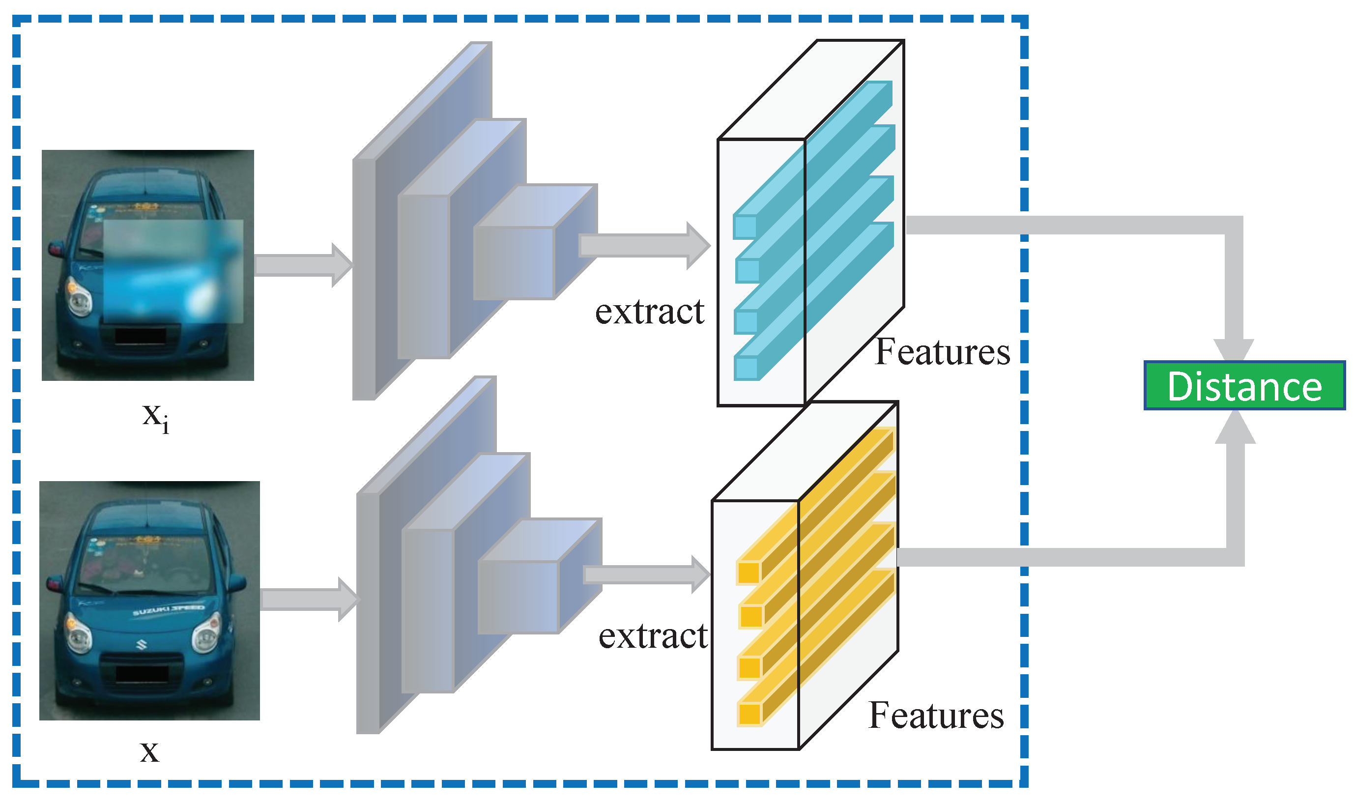
1. Introduction

Vehicle ReID [1] attempts to locate the identity of a specific vehicle in a huge network of cameras quickly. It has been used in a variety of contexts. For starters, vehicle ReID [2] can help police fight crime. Moreover, it can aid city planners in gaining a better understanding of traffic flow. With a strong application background, vehicle ReID is gaining traction in computer vision tasks. Over the last decade, deep learning has become popular and a major method used for computer vision. The research community has been driven to create CNN-based [3] approaches for vehicle ReID tasks.

In order to train a model with good performance throughout the training process, neural networks typically require quite massive amount of data. Data collection and annotation, on the other hand, are quite costly. Moreover, a shortage of data is an obvious stumbling point when building a strong deep neural network. It frequently results in overfitting or poor generalization. Data limitation leads to performance reduction in the field of vehicle ReID as well. Data augmentation [4] is a good method for obtaining extra training samples without having to collect and annotate more data. Common augmentation methods typically generate more training samples by data warping. Moreover, data warping includes random erasing [5], adversarial training [6], geometric and color transformations, and neural style transfer [7].

Unlike previous traditional methods [8], we propose a novel data augmentation strategy that increases the complexity rather than the number of samples in a dataset. In particular, our method blends traditional augmentation method with deep learning technology. A general framework has been attempted in our previous work [9] to exercise this idea. To make the framework more efficient, we adopt the architecture and reorder some of the modules. We introduce a filter matrix to blur the local region of an image sample in order to increase the difficulty of network learning. First, we use a local region selection and a light weight neural network to learn the filter matrix for further data augmentation. Here, we define this light weight neural network as the parameter generator network (PGN). The special purpose of this step is to retain essential information while increasing the difficulty of identification. Second, an adversarial module is employed in our framework. This module includes a recognizer and a parameter generator, as previously mentioned. The recognizer is intended for identifying the vehicles in datasets that belong to the same identity. The parameter generator (PGN), on the other hand, generates augmented image samples. However, the identities of these augmented images are not necessarily the same as the identities of the original images. Thus, the recognizer and PGN form an adversarial module. The two modules compete with each other and strike a balance between the consistency of vehicle identities and the variation of transformed samples. The results of augmented images are depicted in Figure 1. Extensive experiments prove that our framework has excellent generalizability.

For validation, three datasets, i.e., VeRi-776 [10], VehicleID [11], and VERI-Wild [12], are subjected to a series of asymptotic ablation experiments. Our experiments show that the framework proposed greatly surpass the baseline and other previous methods.

Our contributions are summed up as follows:

• A data augmentation method that combines traditional data augmentation and deep learning technology;
• A deep learning framework that combines region location selection, local blur transformation, and an adversarial framework;
• Rather than adding more samples, the dataset is expanded by making the data samples harder. The original structure of the dataset is retained;
• The proposed framework optimizes both the data augmentation and the recognition model without any fine-tuning. The augmented samples are created by dynamic learning.

The rest of this paper is organized as follows. Section 2 presents related work with respect to our research. Our method is then elaborated in Section 3, including some algorithm details and framework descriptions. Section 4 involves the experiments and addresses some qualitative analysis. At the end, we provide some conclusions in Section 5.

2. Related Work

2.1. Vehicle Re-Identification (ReID)

Vehicle ReID [13,14] has extensive research and important applications in computer vision. With the rapid development of deep learning techniques, using neural networks has become mainstream for vehicle ReID. Vehicle ReID [15] requires robust and discriminative image representation. Liu et al. [10] proposed a fusion of multiple features, e.g., colors, textures, and deep learned semantic features. Furthermore, Liu et al. proposed a large-scale benchmark VeRi-776 and improved the performance of their previous model FACT with a Siamese network for license plate recognition and spatio-temporal properties [10]. Deep joint discriminative learning (DJDL) for extracting exclusivity features was proposed by Li et al. [16]. They demonstrated a pipeline that mapped vehicle images into a vector space using deep relative distance learning (DRDL), and the similarity of the two vehicles could be referred to the distance. Wang et al. [17] extracted orientation information from 20 key-point locations of vehicles and presented an orientation-invariant feature-embedding module. Wei et al. [18] introduced a recurrent neural network-based hierarchical attention (RNN-HA) network for vehicle ReID, which incorporated a large number of attributes. Bai et al. [19] suggested a group sensitive triplet embedding strategy to model interclass differences, which Bai et al. [19] found to be effective. He et al. [20] recently investigated both local and global representations to offer a valid learning framework for vehicle re-ID; however, their method is labor-intensive because it is dependent on the labeled components.

Although the previously mentioned vehicle ReID methods differ in some ways, they all need a large number of image samples. However, acquiring data is time-consuming and labor-intensive. Moreover, data augmentation is a very good way to solve this problem.

2.2. Generative Adversarial Networks (GAN)

Goodfellow et al. [21] have made great achievements in image generation, and there have been many applications [22,23,24,25]. GAN [26] is a deep learning model that has emerged as one of the most promising approaches for unsupervised learning on complex distributions. The original GAN [27] was proposed with a deconvolutional network for generating images from noise and a convolutional network for discriminating real or fake samples. To produce a reasonably good output, the model learns by playing each other through two modules of the framework: the Generative and the Discriminative.

In domains with a lack of image samples, GAN is a potent data augmentation tool [28]. It can help create artificial instances from datasets. Bowles et al. [29] discussed it as a method for extracting extra data from datasets. Denoising convolutional neural networks (DnCNN) [30] and image restoration convolutional neural networks (IRCNN) [31] are two CNN-based approaches. By employing the CNN-based end-to-end transformation, these CNN-based approaches considerably improve the performance of image denoising compared to model-based optimization methods.

However, the images generated by GAN [21] are determined by a random vector, and the results cannot be controlled. To overcome this problem, a conditional version named conditional generative adversarial nets (CGAN) [32] was proposed. CGAN conditions not only the generator but also the discriminator by introducing external cues. Inspired by GAN ideas, we add an adversarial module to the overall framework to effectively generate the augmented samples.

2.3. Data Augmentation

Data augmentation [4] is often used to help avoid overfitting [33]. In vehicle ReID tasks, problems such as view angles, illumination, overlapping shadows, complex backgrounds, and image scaling must be overcome. Nevertheless, there are not many good solutions for addressing data augmentation. It is widely assumed that larger datasets produce better training models. However, due to the manual efforts involved in collecting and labeling data, assembling massive datasets can be a scary task.

In many areas of image research, general augmentation methods such as flipping, rotation, scaling, and perspective transformation [4] are often effective. In the vehicle ReID task, we found that only using normal data augmentation is not sufficient. These methods are not flexible enough and do not fully satisfy the effect of dynamic optimization. Peng et al. [34] augmented samples jointly using adversarial learning and pre-training processes. Ho et al. [35] developed flexible augmentation policy schedules to expedite the search process. Cubuk et al. [36] used reinforcement learning to search the policy for augmentation.

Our new method becomes more advantageous, because it integrates the previously mentioned traditional methods and our deep learning module.

3. Methodology

We propose an adversarial strategy and local blur transformation to make more efficient augmented samples. In this section, the overall structure of the framework (Section 3.1) is described at first. Then, we introduce the two main modules separately—Local Blur Transformation (Section 3.2) and Transformation Adversarial Module (Section 3.3).

3.1. Overall Framework

The suggested framework contains two components, as shown in Figure 2: local blur transformation (LBT) and transformation adversarial module (TAM).

A sample, denoted as x, is input to framework. Firstly, LBT takes input image x and selects one local region. Then, it produces four transformed augmented images $x_1,\cdots ,x_4$, each with a different filter matrix. Finally, given images $x_1,\cdots ,x_4$, TAM chooses the most difficult vehicle among them as the replacement. The most difficult vehicle image has the largest distance from input image x.

TAM consists of PGN and the recognizer. When augmented images $x_1,\cdots ,x_4$ enter the recognizer, the recognizer checks if these image identities still equal to image sample x. The image will be discarded if it no longer belongs to the original identity.

Note that PGN is employed both in LBT and TAM. PGN is used in LBT to supply the parameters of the filter matrix needed for the blur transformation. Meanwhile, in TAM, PGN creates the most difficult augmented sample.

At the end, the most difficult sample selected by TAM replaces the original image as a training sample; then, we proceed to the next iteration.

3.2. Local Blur Transformation (LBT)

LBT determines a local blur region and then generates four augmented samples. This includes three steps: local-region selection (LRS), the parameter generator network (PGN), and blur transformation. LRS produces a rectangle region for blur transformation, and then PGN outputs the weight values for the filter matrix. Finally, we obtain the augmented samples by local blur transformations.

3.2.1. Local-Region Selection (LRS)

LRS is employed to select an interest range from input sample. Algorithm 1 specifically describes the process of selecting a local rectangular region. The ratio of the selected area is initialized between $A_1$ and $A_2$. A reasonable aspect ratio is set up from $R_1$ to $R_2$ to create a selected area that is more square. Specifically, the area ratio, donated as $A_t$, is set up at a range from $A_1\le A_t\le A_2$, and the aspect ratio as $R_t$ satisfies $R_1\le R_t\le R_2$. With $A_t$ and $R_t$, the width $W_t$ and height $H_t$ of the selected region are calculated. Moreover, the top-left corner of the selected region is also determined by random position $P_{x,y}$ such that the region is fully located inside the image. Thus, the local region is finally represented by $(P_{x,y},W_t,H_t)$.

Algorithm 1 Process of Local-Region Selection

Input: image width W; image height H;  area of image A;  ratio of width and height R;  area ratio ranges from $A_1$ to $A_2$;  aspect ratio ranges from $R_1$ to $R_2$. Output: selected rectangle region $(P_{x,y},W_t,H_t)$.   1: repeat   2:  $A_t\leftarrow \mathbf{rand}(A_1,A_2)\times A$   3:  $R_t\leftarrow \mathbf{rand}(R_1,R_2)$   4:  $H_t\leftarrow \sqrt{A_t\times R_t}$   5:  $W_t\leftarrow \sqrt{A_t÷R_t}$   6:  $P_x\leftarrow \mathbf{rand}(0,W)$   7:  $P_y\leftarrow \mathbf{rand}(0,H)$   8: until$P_x+W_t\le W\wedge P_y+H_t\le H$   9: return rectangle region $(P_{x,y},W_t,H_t)$

3.2.2. Parameter Generator Network (PGN)

Once the local region is determined, it enters the PGN. Then, PGN generates the weight of a filter matrix for blur transformation. The parameters, four transformation weights $W_1,\cdots ,W_4$, form the following $3\times 3$ filter matrix.

$$S_1=\left(\begin{array}{ccc}0& W_1& 0\\ W_2& 0& W_4\\ 0& W_3& 0\end{array}\right).$$

(1)

The detailed structure of PGN is shown in 

Table 1. Structure of PGN. $\mathbf{BN}$ means batch normalization and $\mathbf{MP}$ represents $2\times 2$ max pooling. The inputted $1\times h\times w$ image size is generated by LRS.

Description	Dimension
Original	$1\times h\times w$
Con16, Relu, MP	$16\times 16\times 50$
Con64, Relu, MP	$64\times 8\times 25$
Con128, BN, Relu	$128\times 8\times 25$
Con128, Relu, MP	$128\times 4\times 12$
Con64, BN, Relu	$64\times 4\times 12$
Con16, BN, Relu, MP	$16\times 2\times 6$
FLayer	4

. It contains convolutional, pooling, and fully connected layers. In particular, MP donates a max pooling layer, and BN stands for batch normalization. Note that the kernel size, stride, and padding size are, respectively, 3, 1, and 1. At the end, FC layer outputs four parameters, which contribute to another filter matrix.

As shown in Figure 3, we used a filter matrix with the original sample to synthesize the augmented blur image; see Section 3.2.3 for more details. To produce the four augmented samples, the other three filter matrices $S_2$, $S_3$, and $S_4$ must be created. By rotating the positions of the weight parameters clockwise, we obtain the following filter matrices.

$$S_2=\left(\begin{array}{ccc}0& W_2& 0\\ W_3& 0& W_1\\ 0& W_4& 0\end{array}\right),S_3=\left(\begin{array}{ccc}0& W_3& 0\\ W_4& 0& W_2\\ 0& W_1& 0\end{array}\right),S_4=\left(\begin{array}{ccc}0& W_4& 0\\ W_1& 0& W_3\\ 0& W_2& 0\end{array}\right).$$

(2)

Finally, we utilize the four filter matrices $S_1,\cdots ,S_4$ with original sample x to transform four augmented samples $x_1,\cdots ,x_4$. The four augmented samples are made by LBT. Our innovation lies in the generation of transformation parameters by using a neural network, which greatly improves the efficiency of the framework.

3.2.3. Blur Transformation

When the filter matrices $S_1,\cdots ,S_4$ are generated, blur transformation is employed to change the original sample x to four augmented samples $x_1,\cdots ,x_4$. Blur transformation transforms the original image to a new augmented image, as shown in Figure 3.

We obtain the filter matrix by using the four weights obtained by PGN, placing them into the corresponding positions of a $3\times 3$ filter matrix and filling the remaining positions of the matrix with 0. Then, we obtain each blurred pixel by making a dot product of this matrix and the $3\times 3$ window anchored at the pixel of the original local image. As a result, we obtain the local blur image. In order to compensate for the extra margin of the local blur image, we add padding to the outer edge of the original local image and fill it all the positions with 0, as shown in Figure 4. After padding, the result will be a blurred and uniformly sized output image according to the matrix’s sliding calculation.

In summary, the blur transformation calculation formula is carried out specifically as follows. Suppose the original image is $H\times W$; then, the pixel value matrix of the original image is o, the pixel value filter matrix is f, and the transformed pixel value is t. We then obtain t from o and f by Equation (3), where $0\le x\le W$ and $0\le y\le H$.

$$t[x,y]=\sum _{l=0}^2\sum _{k=0}^{2}o[x+k,y+l]\times f[k,l].$$

(3)

In particular, for the filtered structure, there may be negative values or values greater than 255. For this case, we truncate them directly between 0 and 255. For negative ones, the absolute value is taken to ensure that the result of the operation is positive.

$$t[x,y]\leftarrow \left|t\right[x,y\left]\right|mod256.$$

(4)

3.3. Transformation Adversarial Module (TAM)

The goal of TAM is to be able to generate augmented images that are hard enough while keeping the sample’s identity constant. If a transformed image looses its vehicle identity, we thought that it had incorporated too much noise and discarded it from the augmented dataset. The experimental results showed that this form of filtering was quite effective. TAM is made up of three components: PGN, the recognizer, and learning target selection. Due to the adversarial module, PGN will dynamically optimize itself. The structure of TAM is shown in the green part of Figure 2. Before explaining the individual components of TAM, we elaborate the algorithm of TAM in Algorithm 2.

The algorithm contains PGN and the recognizer. PGN outputs the paramter of the filter matrix for further augmentation. The recognizer ensures that the identity of image is unchanged. The roles of PGN and the recognizer are competitive: one is to make the sample as deformed as possible, and the other is to ensure that the identity is lost after excessive augmentation.

Algorithm 2 Adversarial process of PGN and the recognizer

Input: selected rectangle region A, original image x Output: updated ${\mathbf{PGN}}^{\prime }$   1: parameter $W_1,W_2,W_3,W_4$ is abtained from PGN: $W_1,W_2,W_3,W_4=\mathbf{PGN}\left(A\right)$   2: form a $3\times 3$ filter matrix $S_1$ by these four parameters $W_1,W_2,W_3,W_4$, then follow the clockwise and fill in the four weight $W_1,W_2,W_3,W_4$ in the corresponding positions to generate the other three filter matrix $S_2,S_3,S_4$   3: finally, obtain augmented images $x_1,x_2,x_3,x_4$ based on $S_1,S_2,S_3,S_4$:   4: recognize image: $\mathit{Reg}\leftarrow \mathbf{Recognizer}\left(x\right)$   5: for  $1\le i\le 4$  do   6:  $x_i\leftarrow \mathbf{BT}(x,S_i)$   7:  recognize image: ${\mathit{Reg}}_i\leftarrow \mathbf{Recognizer}\left(x_i\right)$   8:  if $\mathit{ID}\left[{\mathit{Reg}}_i\right]=\mathit{ID}\left[\mathit{Reg}\right]$ then   9:   ${\Delta }_i\leftarrow measure difficulty by distance between{\mathit{Reg}}_{i}and\mathit{Reg}$   10:  end if   11: end for   12: $i\leftarrow {arg\; max}_i\left\{{\Delta }_i\mid {\Delta }_{i}isdefined,1\le i\le 4\right\}$   13: if $i\mathrm{is} \mathrm{defined}$ then   14:  ${\mathbf{PGN}}^{\prime }$ = update $\mathbf{PGN}$ with $S_i$   15: else   16:  ${\mathbf{PGN}}^{\prime }$ = $\mathbf{PGN}$   17: end if

3.3.1. Recognizer

The recognizer is intended for retaining the sample’s identity. It calculates the likelihood that augmented samples belong to the same identity by comparing their vector-space distances. The greater the probability, the more likely it is that they are members of the same vehicle. The recognizer is reconstructed on the basis of ResNet50 [37]. ResNet50 is a pre-trained classification network on the ImageNet [38] dataset. It is a proven good feature extraction network. ImageNet [39], containing over 20,000 different categories, is a very good dataset in the field of computer visual research. After pre-training ResNet50 on ImageNet, we then slightly modified the network’s structure, resulting in our recognizer.

Since we compare the spatial distance as a metric, the recognizer is not affected by any form of ID losses. Shi et al. [40], for example, used the CTC loss [41] for convolutional recurrent neural networks, and attentional decoders [42,43] are guided by the cross-entropy loss. As a result, our framework is amenable to various recognizers. In the following experiments, we demonstrate the overall framework’s adaptability.

Specifically, we used the recognizer to combine the augmented samples with the original sample to determine if they have the same classification identification. If the identification of an augmented sample is different, it will be abandoned immediately. Otherwise, they are saved for further steps.

3.3.2. Learning Target Selection

The most difficult augmented sample will be kept with the help of learning target selection. Meanwhile, the selected filter matrix will update the PGN parameters in turn.

As shown in Figure 5, the distances are calculated between images $x_1,\cdots ,x_4$ and the original sample, x. The most difficult augmented image with the largest feature distance will be selected at the end. Using this strategy, we choose the augmented one with the largest distance and optimized PGN with the corresponding parameters. As a result, we select the augmented image sample $x^{\prime }$ to replace the original x.

Based on the distance, we choose the largest filter matrix from $S_1,\cdots ,S_4$ and form vector $\overrightarrow{S^r}$ in turn. Note that the PGN is a neural network; thus, the role of the loss is crucial. The loss is described in Equation (5), and $\overrightarrow{S_1}$ represents the predicted value, while $\overrightarrow{S^r}$ represents the actual value. Moreover, $\overrightarrow{\alpha }$ is a hyperparameter that controls the loss in a flexible manner.

$$Loss\leftarrow f(\overrightarrow{S^r},\overrightarrow{S_1},\overrightarrow{\alpha })$$

(5)

4. Experiment and Explanation

In this section, we conduct a series of experiments in order to demonstrate the performance of the proposed methods.

4.1. Datasets

In order to explore the vehicle ReID problem, a number of datasets have been introduced in the last few years. A dataset should include enough data so that a vehicle ReID model can learn intra-class variations. It should also include a large amount of annotated data collected from a large network of cameras.

4.1.1. VeRi-776

These dataset vehicles were all taken in a natural state. Each image of a vehicle is recorded from numerous angles with different illuminations and resolutions, resulting in a dataset of 50,000 photographs of 776 automobiles. Furthermore, vehicle license plates and spatial temporal relationships are marked for all vehicle tracks. The dataset is commonly utilized in the V-reID problem due to its high recurrence rate and the vast number of vehicle photos recorded with varied features.

4.1.2. VehicleID

VehicleID has 221,763 photos of 26,267 automobiles, with the majority of the photographs being front and rear views. With a total of 250 manufacturer models, each photograph includes extensive information about the vehicle model, as well as vehicle identity and camera number labeling information. In addition, the vehicle’s model information is marked on 90,000 photos of 10,319 automobiles.

4.1.3. VERI-Wild

VERI-Wild was collected in suburban areas and contains 416,314 images of 40,671 vehicles captured by 174 traffic cameras. VERI-Wild vehicles are captured without excessive restrictions and in a much richer scenario where the vehicles are located, and the vehicle images are captured over a long time span with significant changes in lighting and weather. The training set consists of 277,797 images (30,671 vehicles) and the test set consists of 138,517 images (10,000 vehicles).

4.2. Implementation

We resize the image samples to $320\times 320$ at the begining. To verify the framework performance, we use the same settings as baseline [44]. As the backbone feature network, ResNet50 [45] is used. As shown in Figure 6, soft margin triplet loss [46] occurs training. Moreover, the SGD [47] is adopted as the optimizer. In addition, the initial learning rate begins at ${10}^{-2}$ and gradually decreases to ${10}^{-3}$ after the first ten epochs. At the 40th and 70th epoch, it decays to ${10}^{-3}$ and ${10}^{-4}$, respectively. The model runs in a total of 120 epochs at the end.

As a pre-processing module, our framework is added to the of the baseline [44] to perform our experiment. The baseline framework is detail explained in [48,49].

4.3. Ablation Study

We conducted extensive comparative experiments to verify the contribution of the different modules of our framework. As mentioned before, this overall framework consists of LBT and TAM. The two modules, LBT and TAM, can be split further. In other words, our framework can consist of only LBT and also can comprise all modules. Different modules can be composed for ablation experiments.

We then run experiments with two different combinations: LBT and LBT + TAM. The ablation experiments results are shown in

Table 2. Results on the three datasets (%).

Model	VeRi-776		VehicleID						VERI-Wild
			Small		Medium		Large		Small		Medium		Large
	R1	MAP	R1	MAP	R1	MAP	R1	MAP	R1	MAP	R1	MAP	R1	MAP
baseline	95.7	76.6	83.0	77.0	80.7	75.0	79.2	74.0	93.1	72.6	90.5	66.5	86.4	58.5
LBT (Our)	96.7	80.5	84.3	77.8	83.4	77.9	79.9	74.4	91.8	72.7	90.3	66.7	87.6	58.8
LBT + TAM (Our)	96.9	81.6	84.3	77.9	83.5	78.0	79.9	74.6	93.4	72.6	91.1	66.7	87.7	58.8

. Figure 7 shows the augmentation samples results.

4.3.1. Our Model vs. Baseline

We compare the performance on each of the three well-known public datasets. In addition to VeRi-776, the other two dataset, as we know, comprise small, medium, and large datasets. Both in VeRi-776 and other datasets, as shown in Table 2, its performance is superior. Specifically, even if only LBT modules are available, R1 and MAP exceed the baseline by 1.0% and 3.9%, respectively, on VeRi-776. Moreover, we have performed experiments on VehicleID in three groups. The R1 increases 1.3% on the smallVehicleID, 2.7% on the mediumVehicleID, and 0.7% on the largeVehicleID. MAP increased 0.8% on the smallVehicleID, 2.9% on the mediumVehicleID, and 0.4% on the largeVehicleID, respectively.

Even though the performance of those baselines was already excellent before adding TAM, our method is still superior. If we focus more on the average metric, it can be found that LBT and LBT+TAM, respectively, improve the MAP by 3.9% and 5.0% on VeRi-776, 0.8% and 0.9% on smallVehicleID, 2.8% and 3.0% on mediumVehicleID, and 0.4% and 0.6% on largeVehicleID. Note that the MAP has significant enhancements on mediumVehicleID.

As shown in Table 2, LBT and LBT + TAM improved distinctly on VERI-Wild. Note that only when all modules are combined together can the framework’s performance be maximized.

4.3.2. Internal Comparison of Our Model

We know that our modules are flexible and stackable, so let us compare the performance change of our framework when only using the LBT module and when all modules are used. Results shows that MAP improves by 1.1% on VeRi-776 and 0.1%, 0.1%, and 0.2% on VehicleID. Table 2 demonstrates a significant improvement in VERI-Wild. As we can observe, the LBT module is critical to our augmentation framework. However, after adding the TAM module, it works better and renders our framework more complete and automated. For some datasets, the improvement was less obvious, but for VERI-Wild, the improvement was significant.

4.4. Comparison with the Sota

In this part, we compare results against some state-of-the-art methods. As shown in

Table 3. Comparison with the Sota on VeRi-776 (%).

Methods	MAP	R1	R5
Siamese-CNN [50]	54.2	79.3	88.9
FDA-Net [12]	55.5	84.3	92.4
Siamese-CNN+ST [50]	58.3	83.5	90.0
PROVID  [51]	53.4	81.6	95.1
AAVER [52]	66.4	90.2	94.3
BS [53]	67.6	90.2	96.4
CCA [54]	68.0	91.7	94.3
PRN [20]	70.2	92.2	97.9
AGNET [55]	71.6	95.6	96.6
PAMTRI [56]	71.8	92.9	97.0
VehicleX [57]	73.3	95.0	98.0
APAN [57]	73.5	93.3	-
MDL [44]	79.4	90.7	-
Our	81.6	96.9	99.0

,

Table 4. Comparison of the Sota on VehicleID (%).

Methods	Small		Medium		Large
	R1	R5	R1	R5	R1	R5
VAMI [58]	63.1	83.3	52.9	75.1	47.3	70.3
FDA-Net [12]	-	-	59.8	77.1	55.5	74.7
AGNET [55]	71.2	83.8	69.2	81.4	65.7	78.3
AAVER [52]	74.7	93.8	68.6	90.0	63.5	85.6
OIFE [17]	-	-	-	-	67.0	82.9
CCA [54]	75.5	91.1	73.6	86.5	70.1	83.2
PRN [20]	78.4	92.3	75.0	88.3	74.2	86.4
BS [53]	78.8	96.2	73.4	92.6	69.3	89.5
VehicleX [57]	79.8	93.2	76.7	90.3	73.9	88.2
Our	84.3	93.5	83.5	90.6	79.9	86.5

and

Table 5. Comparison of the Sota on VERI-Wild (%).

Methods	Small		Medium		Large
	MAP	R1	MAP	R1	MAP	R1
GoogleNet [59]	24.3	57.2	24.2	53.2	21.5	44.6
FDA-net [12]	35.1	64.0	29.8	57.8	22.8	49.4
MLSL [60]	46.3	86.0	42.4	83.0	36.6	77.5
AAVER [52]	62.2	75.8	53.7	68.2	41.7	58.7
BS [53]	70.0	84.2	62.8	78.2	51.6	70.0
UMTS [61]	72.7	84.5	-	-	-	-
Our	72.9	93.4	66.7	91.1	58.8	87.7

, our method is also significantly superior compared to other methods. The performance results convincingly validate the effectiveness of our approach and further show that the individual modules in the framework are capable of incremental performance improvements. It is worth mentioning that, on VeRi-776, it exceeds the second-best method in MAP accuracy by 2.2%, and it also performs well on the other datasets. Our methods are also very advantageous compared to the best methods currently available.

4.5. Visualization of our Method

Figure 8 shows the process of local blur transformation clearly. We visualize the augmented results of orig- To show our method more clearly, we have created a few figures. On the dataset related to our experiments, four temporary augmented images were generated during the learning process, which we also show in Figure 9. As we can observe, the left column comrpise the original samples, and the right column comprise the augmented images.

From the results of these visualizations, it is clear that although parts of the images have been blurred, most of the features of these vehicles have been retained. Finally, we automatically selected the most suitable image to replace the original one, and the network’s performance is gradually optimized.

5. Conclusions

In this paper, we propose a novel method for augmenting sample data in vehicle ReID. A local blur transformation and an adversarial module were employed to ensure that as much noise information as possible was added to the image sample while preserving the structure of the training datasets. We increase the complexity rather than the number of samples. Because of this advantage, our method can be used as a pre-processing layer in other deep learning systems, broadening its application potential.

Unlike the previous framework, we target the local regions of the images and use convolutional operations to blur them to increase the difficulty of network, thus improving the performance of the network. In future work, we will further improve the framework by adding an attention mechanism to identify local regions more purposefully and make the model more efficient.

Based on the tradeoff between algorithm performance and resource overhead cost, the weight of the filter matrix for blur transformation has only four non-zero values. In subsequent research studies, we will consider more effective methods for further optimizing the balance, and we will perform more experiments for verification. We also have plans to perform more experiments in order to combine more baselines in order to verify the generality of our framework.

References

- Li, J.; Cong, Y.; Zhou, L.; Tian, Z.; Qiu, J. Super-resolution-based part collaboration network for vehicle re-identification. World Wide Web 2022, 1–20. [Google Scholar] [CrossRef]
- Wang, L.; Dai, L.; Bian, H.; Ma, Y.; Zhang, J. Concrete cracking prediction under combined prestress and strand corrosion. Struct. Infrastruct. Eng. 2019, 15, 285–295. [Google Scholar] [CrossRef]
- Li, Y.; Hao, Z.; Lei, H. Survey of convolutional neural network. J. Comput. Appl. 2016, 36, 2508–2515. [Google Scholar]
- Shorten, C.; Khoshgoftaar, T.M. A survey on image data augmentation for deep learning. J. Big Data 2019, 6, 60. [Google Scholar] [CrossRef]
- Zhong, Z.; Zheng, L.; Kang, G.; Li, S.; Yang, Y. Random Erasing Data Augmentation. Proc. Aaai Conf. Artif. Intell. 2017, 34. [Google Scholar] [CrossRef]
- Tramèr, F.; Kurakin, A.; Papernot, N.; Goodfellow, I.; Boneh, D.; McDaniel, P. Ensemble adversarial training: Attacks and defenses. arXiv 2017, arXiv:1705.07204. [Google Scholar]
- Jing, Y.; Yang, Y.; Feng, Z.; Ye, J.; Yu, Y.; Song, M. Neural style transfer: A review. IEEE Trans. Vis. Comput. Graph. 2019, 26, 3365–3385. [Google Scholar] [CrossRef] [Green Version]
- Xia, R.; Chen, Y.; Ren, B. Improved anti-occlusion object tracking algorithm using Unscented Rauch-Tung-Striebel smoother and kernel correlation filter. J. King Saud-Univ. Comput. Inf. Sci. 2022. [Google Scholar] [CrossRef]
- Chen, Y.; Ke, W.; Lin, H.; Lam, C.T.; Lv, K.; Sheng, H.; Xiong, Z. Local perspective based synthesis for vehicle re-identification: A transformation state adversarial method. J. Vis. Commun. Image Represent. 2022, 103432. [Google Scholar] [CrossRef]
- Liu, X.; Liu, W.; Ma, H.; Fu, H. Large-scale vehicle re-identification in urban surveillance videos. In Proceedings of the 2016 IEEE International Conference on Multimedia and Expo (ICME), Seattle, WA, USA, 11–15 July 2016; pp. 1–6. [Google Scholar]
- Liu, H.; Tian, Y.; Yang, Y.; Pang, L.; Huang, T. Deep relative distance learning: Tell the difference between similar vehicles. In Proceedings of the IEEE Conference on Computer Vision and Pattern Recognition, Las Vegas, NV, USA, 27–30 June 2016; pp. 2167–2175. [Google Scholar]
- Lou, Y.; Bai, Y.; Liu, J.; Wang, S.; Duan, L. Veri-wild: A large dataset and a new method for vehicle re-identification in the wild. In Proceedings of the IEEE Conference on Computer Vision and Pattern Recognition, Long Beach, CA, USA, 15–20 June 2019; pp. 3235–3243. [Google Scholar]
- Hu, Z.; Xu, Y.; Raj, R.S.P.; Cheng, X.; Sun, L.; Wu, L. Vehicle re-identification based on keypoint segmentation of original image. Appl. Intell. 2022, 1–17. [Google Scholar] [CrossRef]
- Ning, X.; Gong, K.; Li, W.; Zhang, L.; Bai, X.; Tian, S. Feature refinement and filter network for person re-identification. IEEE Trans. Circuits Syst. Video Technol. 2020, 31, 3391–3402. [Google Scholar] [CrossRef]
- Zhang, J.; Feng, W.; Yuan, T.; Wang, J.; Sangaiah, A.K. SCSTCF: Spatial-channel selection and temporal regularized correlation filters for visual tracking. Appl. Soft Comput. 2022, 118, 108485. [Google Scholar] [CrossRef]
- Li, Y.; Li, Y.; Yan, H.; Liu, J. Deep joint discriminative learning for vehicle re-identification and retrieval. In Proceedings of the 2017 IEEE International Conference on Image Processing (ICIP), Beijing, China, 17–20 September 2017; pp. 395–399. [Google Scholar]
- Wang, Z.; Tang, L.; Liu, X.; Yao, Z.; Yi, S.; Shao, J.; Yan, J.; Wang, S.; Li, H.; Wang, X. Orientation invariant feature embedding and spatial temporal regularization for vehicle re-identification. In Proceedings of the IEEE International Conference on Computer Vision, Venice, Italy, 22–29 October 2017; pp. 379–387. [Google Scholar]
- Wei, X.S.; Zhang, C.L.; Liu, L.; Shen, C.; Wu, J. Coarse-to-fine: A RNN-based hierarchical attention model for vehicle re-identification. In Proceedings of the Asian Conference on Computer Vision, Perth, Australia, 2–6 December 2018; Springer: Berlin/Heidelberg, Germany, 2018; pp. 575–591. [Google Scholar]
- Bai, Y.; Lou, Y.; Gao, F.; Wang, S.; Wu, Y.; Duan, L.Y. Group-sensitive triplet embedding for vehicle reidentification. IEEE Trans. Multimed. 2018, 20, 2385–2399. [Google Scholar] [CrossRef]
- He, B.; Li, J.; Zhao, Y.; Tian, Y. Part-regularized near-duplicate vehicle re-identification. In Proceedings of the IEEE Conference on Computer Vision and Pattern Recognition, Long Beach, CA, USA, 15–20 June 2019; pp. 3997–4005. [Google Scholar]
- Goodfellow, I.; Pouget-Abadie, J.; Mirza, M.; Xu, B.; Warde-Farley, D.; Ozair, S.; Courville, A.; Bengio, Y. Generative adversarial nets. Adv. Neural Inf. Process. Syst. 2014, 27, 2672–2680. [Google Scholar]
- Zhou, T.; Tulsiani, S.; Sun, W.; Malik, J.; Efros, A.A. View synthesis by appearance flow. In Proceedings of theEuropean Conference on Computer Vision, Amsterdam, The Netherlands, 11–14 October 2016; Springer: Berlin/Heidelberg, Germany, 2016; pp. 286–301. [Google Scholar]
- Isola, P.; Zhu, J.Y.; Zhou, T.; Efros, A.A. Image-to-image translation with conditional adversarial networks. In Proceedings of the IEEE Conference on Computer Vision and Pattern Recognition, Honolulu, HI, USA, 21–26 July 2017; pp. 1125–1134. [Google Scholar]
- Johnson, J.; Alahi, A.; Fei-Fei, L. Perceptual losses for real-time style transfer and super-resolution. In Proceedings of the European Conference on Computer Vision, Amsterdam, The Netherlands, 11–14 October 2016; Springer: Berlin/Heidelberg, Germany, 2016; pp. 694–711. [Google Scholar]
- Odena, A.; Olah, C.; Shlens, J. Conditional image synthesis with auxiliary classifier gans. In Proceedings of the International Conference on Machine Learning, Sydney, NSW, Australia, 6–11 August 2017; pp. 2642–2651. [Google Scholar]
- Tatarchenko, M.; Dosovitskiy, A.; Brox, T. Multi-view 3d models from single images with a convolutional network. In Proceedings of the European Conference on Computer Vision, Amsterdam, The Netherlands, 11–14 October 2016; Springer: Berlin/Heidelberg, Germany, 2016; pp. 322–337. [Google Scholar]
- Zhou, Y.; Shao, L. Cross-view GAN based vehicle generation for re-identification. In Proceedings of the British Machine Vision Conference, London, UK, 4–7 September 2017. [Google Scholar]
- Bodnar, C. Text to image synthesis using generative adversarial networks. arXiv 2018, arXiv:1805.00676. [Google Scholar]
- Bowles, C.; Chen, L.; Guerrero, R.; Bentley, P.; Gunn, R.; Hammers, A.; Dickie, D.A.; Hernández, M.V.; Wardlaw, J.; Rueckert, D. Gan augmentation: Augmenting training data using generative adversarial networks. arXiv 2018, arXiv:1810.10863. [Google Scholar]
- Zhang, K.; Zuo, W.; Chen, Y.; Meng, D.; Zhang, L. Beyond a gaussian denoiser: Residual learning of deep cnn for image denoising. IEEE Trans. Image Process. 2017, 26, 3142–3155. [Google Scholar] [CrossRef] [PubMed] [Green Version]
- Zhang, K.; Zuo, W.; Gu, S.; Zhang, L. Learning deep CNN denoiser prior for image restoration. In Proceedings of the IEEE Conference on Computer Vision and Pattern Recognition, Honolulu, HI, USA, 21–26 July 2017; pp. 3929–3938. [Google Scholar]
- Mirza, M.; Osindero, S. Conditional generative adversarial nets. arXiv 2014, arXiv:1411.1784. [Google Scholar]
- Ruder, S. An overview of multi-task learning in deep neural networks. arXiv 2017, arXiv:1706.05098. [Google Scholar]
- Peng, X.; Tang, Z.; Yang, F.; Feris, R.S.; Metaxas, D. Jointly optimize data augmentation and network training: Adversarial data augmentation in human pose estimation. In Proceedings of the IEEE Conference on Computer Vision and Pattern Recognition, Salt Lake City, UT, USA, 18–23 June 2018; pp. 2226–2234. [Google Scholar]
- Ho, D.; Liang, E.; Chen, X.; Stoica, I.; Abbeel, P. Population based augmentation: Efficient learning of augmentation policy schedules. In Proceedings of the International Conference on Machine Learning, Long Beach, CA, USA, 9–15 June 2019; pp. 2731–2741. [Google Scholar]
- Cubuk, E.D.; Zoph, B.; Mane, D.; Vasudevan, V.; Le, Q.V. Autoaugment: Learning augmentation strategies from data. In Proceedings of the IEEE/CVF Conference on Computer Vision and Pattern Recognition, Long Beach, CA, USA, 15–20 June 2019; pp. 113–123. [Google Scholar]
- He, K.; Zhang, X.; Ren, S.; Sun, J. Deep residual learning for image recognition. In Proceedings of the IEEE Conference on Computer Vision and Pattern Recognition, Las Vegas, NV, USA, 27–30 June 2016; pp. 770–778. [Google Scholar]
- Krizhevsky, A.; Sutskever, I.; Hinton, G.E. Imagenet classification with deep convolutional neural networks. Adv. Neural Inf. Process. Syst. 2012, 25, 1097–1105. [Google Scholar] [CrossRef]
- Deng, J.; Dong, W.; Socher, R.; Li, L.J.; Li, K.; Fei-Fei, L. Imagenet: A large-scale hierarchical image database. In Proceedings of the 2009 IEEE Conference on Computer Vision and Pattern Recognition, Miami, FL, USA, 20–25 June 2009; pp. 248–255. [Google Scholar]
- Shi, B.; Bai, X.; Yao, C. An end-to-end trainable neural network for image-based sequence recognition and its application to scene text recognition. IEEE Trans. Pattern Anal. Mach. Intell. 2016, 39, 2298–2304. [Google Scholar] [CrossRef] [PubMed] [Green Version]
- Graves, A.; Fernández, S.; Gomez, F.; Schmidhuber, J. Connectionist temporal classification: Labelling unsegmented sequence data with recurrent neural networks. In Proceedings of the 23rd International Conference on Machine Learning, Pittsburgh, PA, USA, 25–29 June 2006; pp. 369–376. [Google Scholar]
- Luo, C.; Jin, L.; Sun, Z. A multi-object rectified attention network for scene text recognition. arXiv 2019, arXiv:1901.03003. [Google Scholar] [CrossRef]
- Shi, B.; Yang, M.; Wang, X.; Lyu, P.; Yao, C.; Bai, X. Aster: An attentional scene text recognizer with flexible rectification. IEEE Trans. Pattern Anal. Mach. Intell. 2018, 41, 2035–2048. [Google Scholar] [CrossRef] [PubMed]
- He, S.; Luo, H.; Chen, W.; Zhang, M.; Zhang, Y.; Wang, F.; Li, H.; Jiang, W. Multi-domain learning and identity mining for vehicle re-identification. In Proceedings of the IEEE/CVF Conference on Computer Vision and Pattern Recognition Workshops, Seattle, WA, USA, 13–19 June 2020; pp. 582–583. [Google Scholar]
- Jung, H.; Choi, M.K.; Jung, J.; Lee, J.H.; Kwon, S.; Young Jung, W. ResNet-based vehicle classification and localization in traffic surveillance systems. In Proceedings of the IEEE Conference on Computer Vision and Pattern Recognition Workshops, Seattle, WA, USA, 14–19 June 2017; pp. 61–67. [Google Scholar]
- Yuan, Y.; Chen, W.; Yang, Y.; Wang, Z. In defense of the triplet loss again: Learning robust person re-identification with fast approximated triplet loss and label distillation. In Proceedings of the IEEE/CVF Conference on Computer Vision and Pattern Recognition Workshops, Seattle, WA, USA, 13–19 June 2020; pp. 354–355. [Google Scholar]
- Zhang, S.; Choromanska, A.; LeCun, Y. Deep learning with elastic averaging SGD. arXiv 2014, arXiv:1412.6651. [Google Scholar]
- Luo, H.; Gu, Y.; Liao, X.; Lai, S.; Jiang, W. Bag of tricks and a strong baseline for deep person re-identification. In Proceedings of the IEEE/CVF Conference on Computer Vision and Pattern Recognition Workshops, Long Beach, CA, USA, 16–17 June 2019. [Google Scholar]
- Luo, H.; Jiang, W.; Gu, Y.; Liu, F.; Liao, X.; Lai, S.; Gu, J. A strong baseline and batch normalization neck for deep person re-identification. IEEE Trans. Multimed. 2019, 22, 2597–2609. [Google Scholar] [CrossRef] [Green Version]
- Shen, Y.; Xiao, T.; Li, H.; Yi, S.; Wang, X. Learning deep neural networks for vehicle re-id with visual-spatio-temporal path proposals. In Proceedings of the IEEE International Conference on Computer Vision, Venice, Italy, 22–29 October 2017; pp. 1900–1909. [Google Scholar]
- Liu, X.; Liu, W.; Mei, T.; Ma, H. Provid: Progressive and multimodal vehicle reidentification for large-scale urban surveillance. IEEE Trans. Multimed. 2017, 20, 645–658. [Google Scholar] [CrossRef]
- Khorramshahi, P.; Kumar, A.; Peri, N.; Rambhatla, S.S.; Chen, J.C.; Chellappa, R. A dual-path model with adaptive attention for vehicle re-identification. In Proceedings of the IEEE International Conference on Computer Vision, Seoul, Korea, 27 October–2 November 2019; pp. 6132–6141. [Google Scholar]
- Kuma, R.; Weill, E.; Aghdasi, F.; Sriram, P. Vehicle re-identification: An efficient baseline using triplet embedding. In Proceedings of the 2019 International Joint Conference on Neural Networks (IJCNN), Budapest, Hungary, 14–19 July 2019; pp. 1–9. [Google Scholar]
- Peng, J.; Jiang, G.; Chen, D.; Zhao, T.; Wang, H.; Fu, X. Eliminating cross-camera bias for vehicle re-identification. Multimed. Tools Appl. 2020, 1–17. [Google Scholar] [CrossRef]
- Zheng, A.; Lin, X.; Li, C.; He, R.; Tang, J. Attributes guided feature learning for vehicle re-identification. arXiv 2019, arXiv:1905.08997. [Google Scholar]
- Tang, Z.; Naphade, M.; Birchfield, S.; Tremblay, J.; Hodge, W.; Kumar, R.; Wang, S.; Yang, X. Pamtri: Pose-aware multi-task learning for vehicle re-identification using highly randomized synthetic data. In Proceedings of the IEEE International Conference on Computer Vision, Seoul, Korea, 27 October–2 November 2019; pp. 211–220. [Google Scholar]
- Yao, Y.; Zheng, L.; Yang, X.; Naphade, M.; Gedeon, T. Simulating content consistent vehicle datasets with attribute descent. arXiv 2019, arXiv:1912.08855. [Google Scholar]
- Zhou, Y.; Shao, L. Aware attentive multi-view inference for vehicle re-identification. In Proceedings of the IEEE Conference on Computer Vision and Pattern Recognition, Salt Lake City, UT, USA, 18–23 June 2018; pp. 6489–6498. [Google Scholar]
- Yang, L.; Luo, P.; Change Loy, C.; Tang, X. A large-scale car dataset for fine-grained categorization and verification. In Proceedings of the IEEE Conference on Computer Vision and Pattern Recognition, Boston, MA, USA, 7–12 June 2015; pp. 3973–3981. [Google Scholar]
- Alfasly, S.; Hu, Y.; Li, H.; Liang, T.; Jin, X.; Liu, B.; Zhao, Q. Multi-Label-Based Similarity Learning for Vehicle Re-Identification. IEEE Access 2019, 7, 162605–162616. [Google Scholar] [CrossRef]
- Jin, X.; Lan, C.; Zeng, W.; Chen, Z. Uncertainty-aware multi-shot knowledge distillation for image-based object re-identification. In Proceedings of the AAAI Conference on Artificial Intelligence, New York, NY, USA, 7–12 February 2020; Volume 34, pp. 11165–11172. [Google Scholar]