Study of the Dynamic Response of a Rigid Runway with Different Void States during Aircraft Taxiing

Abstract

In this study, a set of numerical simulation analysis methods for studying the dynamic response of runway under the action of aircraft taxiing load are presented. An aircraft-runway coupled vibration model was established, and the runway pavement roughness was taken as the vibration excitation source; then, the aircraft taxiing dynamic load was obtained. A three-dimensional finite element model of the runway was established, and the vertical dynamic displacement (VDD) response and its variation law of the runway under different void conditions were studied under the action of the dynamic load of a taxiing aircraft. In addition, using wavelet packet transform, the acceleration signals at different positions of the pavement slab under the sliding load were decomposed into three layers. The relationship among the wavelet packet energy ratio (WPER), the wavelet packet energy entropy (WPEE) of each frequency band, and the void under the pavement slab was obtained. The results show that the established model could quickly and accurately solve the aircraft taxiing dynamic load. In the case of a slight void, the VDDs in the runway center and under the main landing gears had negative exponential and logarithmic relationships with the reduction coefficient of the dynamic elastic modulus of the base layer, respectively. When there was a severe void, the pavement slab was separated from the base layer. The VDDs in the runway center and under the main landing gears were exponentially and linearly related to the slab’s void area, respectively. The vibration signals were extracted at three measuring points, and the wavelet packet energy characteristics of the signals were compared and analyzed. It was found that the WPER and WPEE of the vibration signals in the void area of the slab corner could better reflect the void state of the slab bottom.

1. Introduction

China is one of the countries with the highest number of airports, and civil transport airports completed 907.483 million passengers and 9.777 million aircraft movements in 2021 [1]. While the number and frequency of large aircraft takeoffs and landings continue to rise, the dynamic interaction between aircraft and runways has become more obvious. The void of the cement concrete slab on the runway surface is an issue that easily occurs when the rigid pavement is in service, which aggravates the continuous damage to the runway structure [2] and poses a significant threat to the taxiing safety of the aircraft. The traditional means of void detection can only be carried out when the airport is out of service, and they are labor-intensive, material-intensive, and time-consuming. The runway health condition cannot be known in real time. Therefore, if the relationship between the runway dynamic response and pavement slab void can be obtained under the action of aircraft taxiing load, runway response information can be collected using a reasonable arrangement of sensing devices, and the pavement slab void can be grasped in real time.

In airport engineering research, relevant institutions and researchers have analyzed the pavement response caused by aircraft load and environmental impact by deploying sensors on the runway, thus promoting the development of airport runway health monitoring [3,4,5,6]. Park et al. proposed a method for predicting the performance changes of airport concrete pavement slabs when subjected to temperature and humidity using the measured runway strain response data from sensors [7]. However, measured data are not easily available and can be distorted [8]. Therefore, runway surface unevenness is used as the vibration excitation source to establish the aircraft-runway coupled vibration relationship, which is required for the further analysis of the vibration response. It has been found that runway surface unevenness has a significant effect on the vibration response of the airframe when the aircraft taxies [9]. Taheri et al. proposed a calculation method for the transient response of a runway structure under aircraft moving load by using the aircraft-runway coupled vibration relationship [10]. Many scholars have studied runway structure dynamic response and specific vibration law under complex moving loads by establishing reasonable runway finite element models [11,12], as well as the response of rigid pavement of conventional and snow-melting airports under aircraft loads, temperature loads, and their coupling effects [13]. In a study of the dynamic response of rigid runway pavements, Fu et al. found that the skidding speed significantly affects the dynamic response when skidding lift effects and vibration effects are considered [14]. It is necessary to analyze the lift effect of the aircraft. Meanwhile, according to the stochastic nature of pavement unevenness variation under dual main landing gear, the fuselage rollover rotation needs to be considered when modeling aircraft-runway vibrations.

In concrete road panel debonding identification studies, the traditional falling weight deflectometer (FWD) is still an effective device for road panel void detection [15]. Due to the relative safety, high efficiency, and strong observability of airport pavement defect evaluation conducted using ground-penetrating radar (GPR), GPR has been used to identify different the void states of pavement structures [16,17,18]. It has been shown that the structure’s material properties, stiffness, and other parameters under real-time dynamic loading directly affect the vibration response of the structure [19,20]. When a wavelet packet transform is used to analyze vibration signals, the energy distribution in each frequency band is susceptible to the structural parameters of the vibration source [21,22]. It also has good robustness to noise [23,24]. Therefore, analyzing vibration signals makes it feasible to analyze the structural health condition.

Most of the current studies are focused on the stress, strain, dynamic displacement, and vibration response analyses of healthy roads or runways. The void detection method needs to be performed with the help of an FWD or other instruments. However, there are not many studies focused on the detection of the void of the plate bottom by the mechanical response of the runway during aircraft taxiing. The research method, which is based on the coupled vibration analysis of aircraft-runway excited by the roughness of runway pavement, is described in the second section of this paper. The dynamic load of an aircraft taxiing is calculated using the space state method, and a method for analyzing signals using wavelet packet energy is introduced. The third section focuses on the creation of a rigid runway model with joints, the design of runway models with varying degrees of void, and the effective application of aircraft dynamic load in a finite element model. The fourth section analyzes and discusses the calculation results of runway dynamic response with various degrees of void, as well as the relationship between the wavelet packet energy characteristics of pavement dynamic displacement and vibration signals and the degree of void. Lastly, the fifth section summarizes the findings. The research results can guide the deployment of buried sensors for airport runways, which can directly sense whether the runway contains voids or not by using the interaction between aircraft and runway during nonstop operation.

2. Research Methodology

A time-domain model of runway surface roughness and a four-degrees-of-freedom (4-DOF) aircraft-runway coupled vibration model were established. The former was used as the vibration excitation source, and the state space method was used to solve the aircraft taxiing load. ABAQUS is a commonly used finite element analysis software, which has a wide range of applications. By associating its user subroutine DLOAD and writing the corresponding Fortran language, complex dynamic loads can be applied to the finite element model for calculation and analysis. The dynamic displacement response of the runway structure was studied, and the energy distribution of the vertical vibration acceleration response signal of runway slab based on wavelet packet transform was calculated and analyzed. The research method and steps are shown in Figure 1.

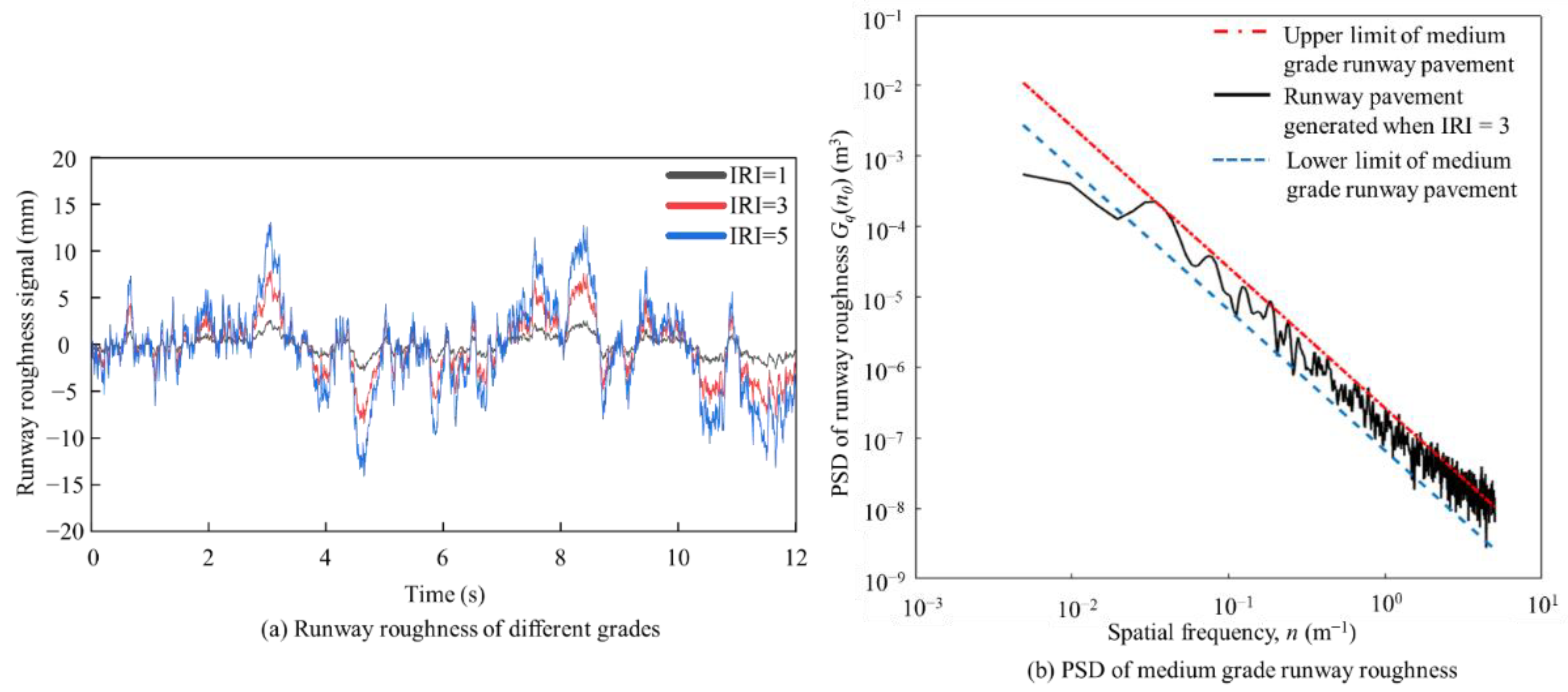
2.1. Runway Pavement Roughness Time-Domain Model

Airport runway pavement roughness is the vertical deviation of the runway surface relative to the ideal plane, which corresponds to the longitudinal roughness of the runway surface [25]. It has been shown that pavement roughness can be considered to obey a normal distribution with zero mean. The pavement roughness’s vertical speed power spectrum density (PSD) is consistent with the white-noise power spectrum. Therefore, the vertical speed input of pavement roughness can be simulated by white noise. Establishing the time-domain model of pavement roughness is feasible using the filtered white noise method [26]. According to the international standard ISO 8608 recommendation [27], the pavement roughness PSD function can be expressed by Equation (1).

$$G_q(n)=G_q(n_0){\left(\frac{n}{n_0}\right)}^{-2},$$

(1)

where n is the spatial frequency (m⁻¹), n₀ is the reference frequency (n₀ = 0.1 m⁻¹), and G_q (n₀) is the pavement PSD at the reference frequency (m³).

The aircraft taxiing speed is v (m/s), and the time frequency is f = vn; then, the PSD function with time as the reference is expressed by Equation (2).

$$G_q(f)=G_q(n_0)n_0{}^2\frac{v}{f^2}.$$

(2)

Considering the actual situation, by introducing a lower cutoff frequency f₀ to the pavement roughness model, Equation (2) can be rewritten as Equation (3).

$$G_q(f)=G_q(n_0)n_0{}^2\frac{v}{{(f+f_0)}^2}.$$

(3)

The filtered white noise method equates the pavement roughness signal q(t) to the first-order linear system response of the unit white-noise signal w(t). The frequency response function of the system is obtained from Equation (4).

$$H(j\omega )=\frac{2\pi n_0\sqrt{G_q(n_0)v}}{j\omega +{\omega }_0}=\frac{2\pi n_0\sqrt{G_q(n_0)v}}{j\omega +2\pi n_{1}v},$$

(4)

where ω is the circular frequency (rad/s), and n₁ is the cutoff frequency of the pavement space (m⁻¹).

The first-order differential equation to establish the pavement roughness using filtered white noise is expressed by Equation (5).

$$\dot{q}(t)=-2\pi f_{0}q(t)+2\pi n_0\sqrt{G_q(n_0)v}w(t),$$

(5)

where the lower cutoff time frequency is f₀ = vn₁, and the filtered white noise pavement roughness time-domain model can be further defined as Equation (6).

$$\dot{q}(t)=-2\pi n_{1}vq(t)+2\pi n_0\sqrt{G_q(n_0)v}w(t).$$

(6)

The general pavement roughness wavelength is from 0.1 to 100 m; hence, the lower cutoff spatial frequency n₁ in the above equation is 0.01 m⁻¹.

The International Roughness Index (IRI) can evaluate airport runway leveling grades [28,29], and the IRI grading criteria are shown in

Table 1. Airport pavement IRI grading standard.

Evaluation Level	Good	Medium	Poor
IRI average (m/km)	<2.0	2.0~4.0	>4.0

.

The corresponding PSD G_q (n₀) is obtained by converting the IRI. According to existing studies, G_q (n₀) and IRI can be interconverted using Equation (7) [30], and the IRI grading criteria and their corresponding power spectral densities are shown in

Table 2. The PSD of different IRI grades.

Road-Surface Evaluation Grade	IRI	Gq (n0) (10−6 m3)
Good	1	1.6436
Medium	2	6.5746
Medium	3	14.7929
Medium	4	26.2985
Poor	5	41.0914

.

$$\mathrm{IRI}=0.78a_0\sqrt{G_q(n_{{}_0})},$$

(7)

where, a₀ = 10³ m^−1.5.

The corresponding module was built in the MATLAB/SIMULINK environment based on Equation (6). A band-limited white-noise output with a unilateral power of 1 was required in the simulation. A bilateral power spectrum was assumed in the SIMULINK band-limited white-noise module [31]; therefore, this module’s noise power spectral density was set to 0.5. According to the sampling theorem, the sampling time of the band-limited white-noise module was set to 1/10u to ensure 10 sampling points per meter, and the band-limited white-noise seed was set to the default value. The process provides the vibration excitation source for the subsequent establishment of the aircraft-runway coupled vibration model.

The time-domain signal of runway pavement roughness was simulated and verified. Figure 2a depicts the generated runway roughness signal when the aircraft taxiing speed was 20 m/s and the IRI values were 1, 3, and 5. The generated pavement with the IRI value of 3 was compared with the standard PSD of the pavement. The upper and lower boundaries were standard power spectral densities with IRI values of 2 and 4, respectively. The results are shown in Figure 2b; the spectrum was located in the mid-grade runway road surface area, which was nearly in line with an actual situation.

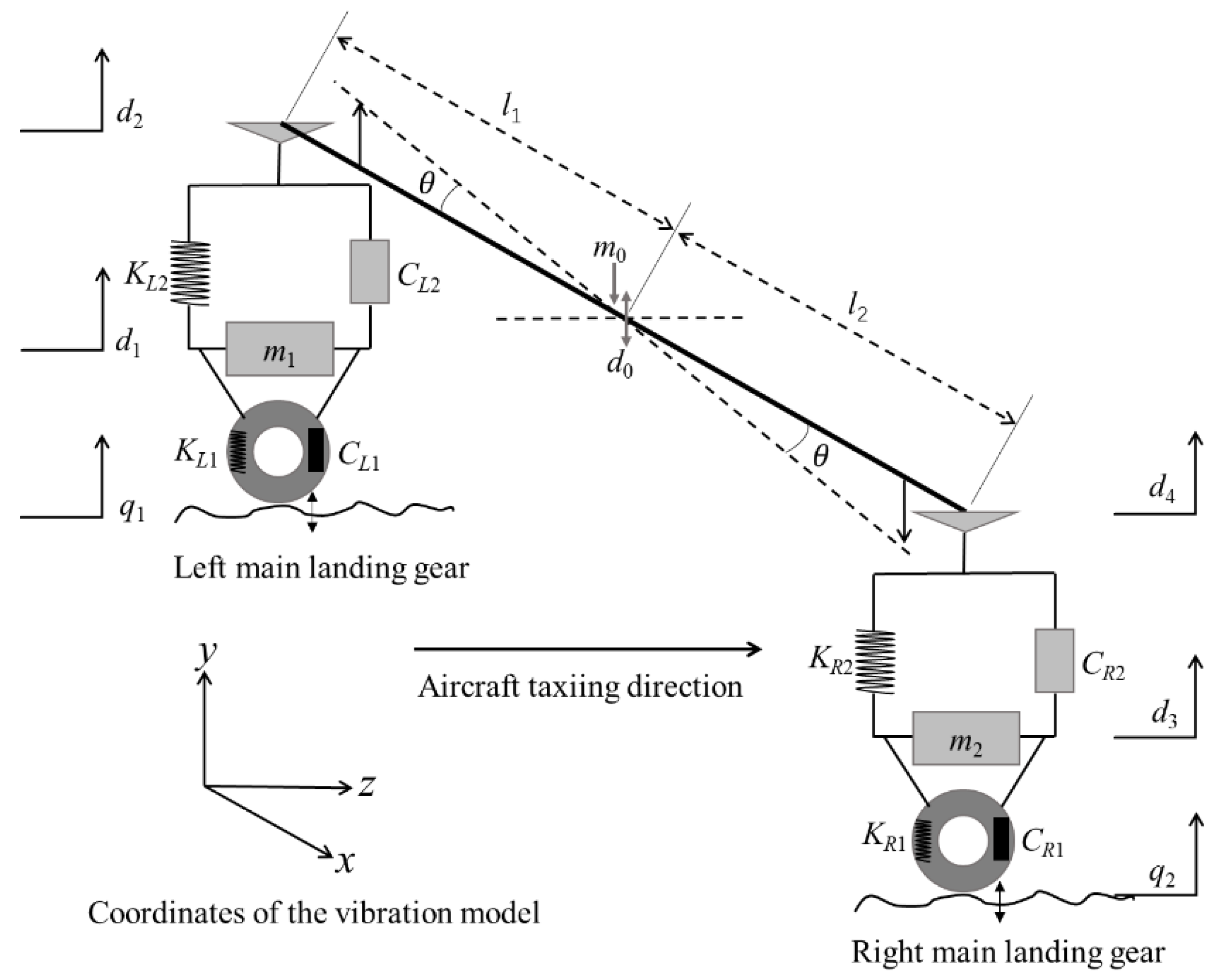
2.2. Establishment of Coupled Vibration Model of Aircraft-Runway

The main landing gear of most civil airliners has an airframe weight distribution coefficient of about 0.95 [32]; thus, only the interaction between the main landing gear of the aircraft and the road surface when bearing 95% of the sprung mass needs to be considered. Thus, the vibration model of the aircraft could also be simplified by dividing the upper sprung mass and the lower unsprung mass. Both the cushioning device of the main landing gears and the tires were treated as consisting of a spring with the corresponding stiffness coefficient and a damping device with the corresponding damping coefficient.

Based on the vertical motion and lateral tilt rotation of the fuselage, the vertical motion of the left landing gear, and the vertical movement of the right landing gear while the aircraft taxies on the runway, a four-degrees-of-freedom aircraft vibration model was established, as shown in Figure 3. For the fuselage, m₀ is the sprung mass of the fuselage, the vertical displacement is d₀, and the lateral tilt rotation inertia and the rotational displacement are I_z and θ (side-turning rotation around the z-axis). For the left and right main landing gears, the unsprung masses are m₁ and m₂, the unsprung mass stiffness values are K_L1 and K_R1, the unsprung mass damping values are C_L1 and C_R1, the sprung mass stiffness values are K_L2 and K_R2, the damping values of sprung mass are C_L2 and C_R2, the vertical displacements at the corresponding fuselage are d₂ and d₄, the vertical displacements of unsprung mass are d₁ and d₃, and the excitations of unsprung mass by runway pavement roughness are q₁ and q₂. The distances from the left and right main landing gears to the z-axis are l₁ and l₂, where l₁ = l₂ = l, while, from the established model, it is known that d₂ = d₀ + l·θ, d₄ = d₀ − l·θ.

The four-degrees-of-freedom vibration balance equation of the aircraft model can be expressed by Equations (8)–(11).

$$m_0{\ddot{d}}_0+K_L{}_2(d_2-d_1)+C_L{}_2({\dot{d}}_2-{\dot{d}}_1)+K_R{}_2(d_4-d_3)+C_R{}_2({\dot{d}}_4-{\dot{d}}_3)=0.$$

(8)

$$m_1{\ddot{d}}_1+K_L{}_2(d_1-d_2)+C_L{}_2({\dot{d}}_1-{\dot{d}}_2)+K_L{}_1(d_1-q_1)+C_L{}_1({\dot{d}}_1-{\dot{q}}_1)=0.$$

(9)

$$m_2{\ddot{d}}_3+K_R{}_2(d_3-d_4)+C_R{}_2({\dot{d}}_3-{\dot{d}}_4)+K_R{}_1(d_3-q_2)+C_R{}_1({\dot{d}}_3-{\dot{q}}_2)=0.$$

(10)

$$I_z\ddot{\theta }+l\left[K_L{}_2(d_2-d_1)+C_L{}_2({\dot{d}}_2-{\dot{d}}_1)\right]-l\left[K_R{}_2(d_4-d_3)+C_R{}_2({\dot{d}}_4-{\dot{d}}_3)\right]=0.$$

(11)

The random dynamic load, F_d, exerted by the left and right landing gears on the runway surface is represented by Equation (12).

$$\left\{\begin{array}{l}{F}_{d1}=K_L{}_1(d_1-q_1)+C_L{}_1({\dot{d}}_1-{\dot{q}}_1)\\ F_{d2}=K_R{}_1(d_3-q_2)+C_R{}_1({\dot{d}}_3-{\dot{q}}_2)\end{array}\right..$$

(12)

Equation (13) expresses lift force F_s generated by the wing when the aircraft taxies.

$$F_s=\frac{1}{2}\rho v^2{c}_{y}s,$$

(13)

where ρ is the air density (kg/m³), v is the speed when the aircraft taxies (m/s), c_y is the lift coefficient, which is considered equal to the lift coefficient corresponding to the aircraft stopping angle (−1°) before taxiing head-up, and s is the wing area (m²).

The sum of the weight of the aircraft assigned to the main landing gear spring load and the weight of the main landing gear is G. The total load, F_t, acting on the runway due to the left and right landing gears during taxiing can be expressed by Equation (14).

$$F_t=F_d+G-F_s=\left\{\begin{array}{l}{F}_{t1}=K_L{}_1(d_1-q_1)+C_L{}_1({\dot{d}}_1-{\dot{q}}_1)+1/2G-F_s\\ F_{t2}=K_R{}_1(d_3-q_2)+C_R{}_1({\dot{d}}_3-{\dot{q}}_2)+1/2G-F_s\end{array}\right..$$

(14)

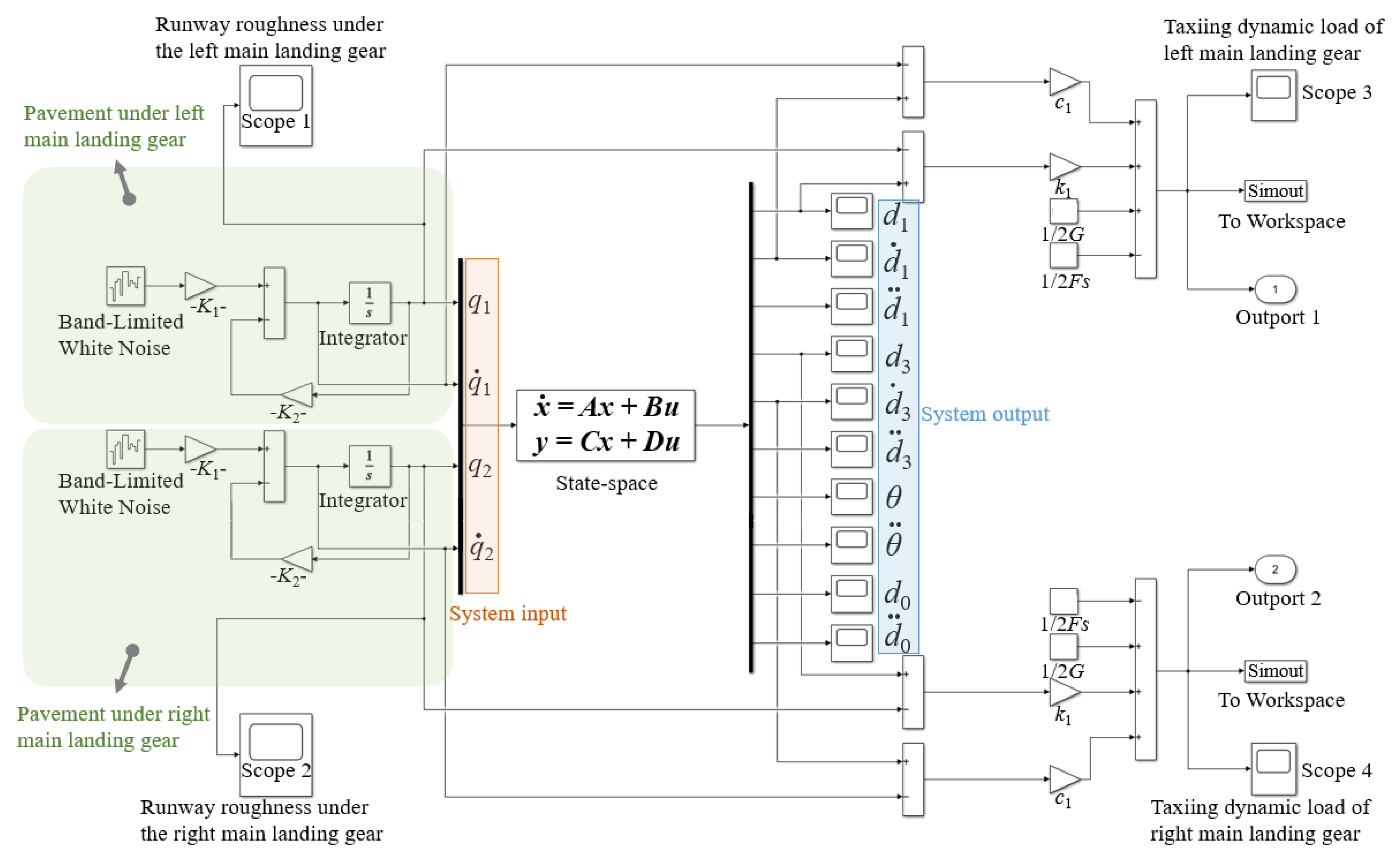
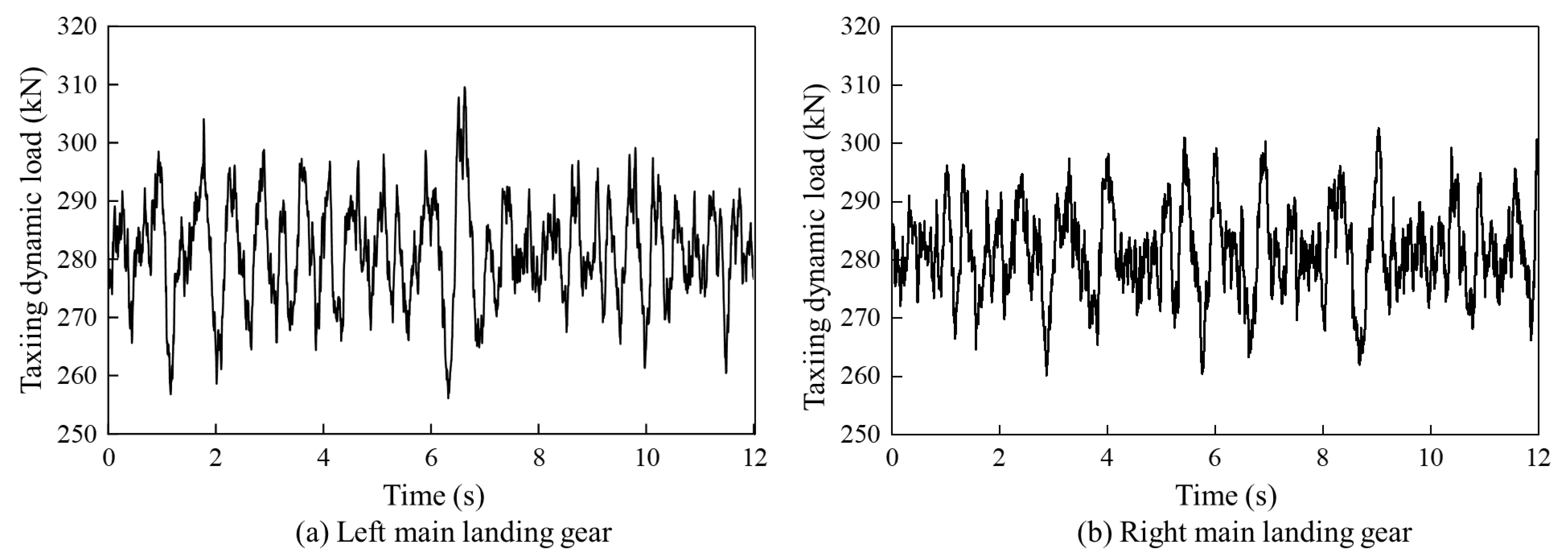
2.3. Aircraft Taxiing Dynamic Loads

In order to solve the aircraft taxiing dynamic load intuitively and conveniently, the aircraft-runway coupled vibration model was simulated by SIMULINK, according to the state space theory [33], and the aircraft vibration balance equation was converted into the form of state equations. The vertical displacements of the sprung masses, the vertical displacements of the unsprung masses of the left and right main landing gears, the lateral tilt rotation displacements, and the first-order derivatives of these parameters were selected as the state vector components, x, which can be expressed by Equation (15).

$$x={(x_1{x}_2{x}_3{x}_4{x}_5{x}_6{x}_7{x}_8)}^{{\rm T}}={(d_1{\dot{d}}_1{d}_3{\dot{d}}_3\theta \dot{\theta }{d}_0{\dot{d}}_0)}^{{\rm T}}.$$

(15)

The output vector, y, is expressed by Equation (16).

$$y={(y_1{y}_2{y}_3{y}_4{y}_5{y}_6{y}_7{y}_8{y}_9{y}_{10})}^{{\rm T}}={(d_1{\dot{d}}_1{\ddot{d}}_1{d}_3{\dot{d}}_3{\ddot{d}}_3\theta \ddot{\theta }{d}_0{\ddot{d}}_0)}^{{\rm T}}.$$

(16)

The runway pavement roughness and its first derivative are represented by the input vector, u, which is expressed by Equation (17).

$$u={(q_1{\dot{q}}_1{q}_2{\dot{q}}_2)}^{{\rm T}}.$$

(17)

The differential equation of the vibrating system can be transformed into a linear state space equation, as shown in Equation (18).

$$\left\{\begin{array}{c}\dot{x}(t)=Ax(t)+Bu(t)\\ y(t)=Cx(t)+Du(t)\end{array}\right.,$$

(18)

where A, B, C, and D matrices; the four matrices can be jointly obtained by Equations (8)–(11) and (15)–(18), as shown in the specific Equations (19)–(22).

$$A=\left[\begin{array}{cccccccc}0& 1& 0& 0& 0& 0& 0& 0\\ -\frac{(K_L{}_1+K_L{}_2)}{m_1}& -\frac{(C_L{}_1+C_L{}_2)}{m_1}& 0& 0& \frac{K_L{}_{2}l}{m_1}& \frac{C_L{}_{2}l}{m_1}& \frac{K_L{}_2}{m_1}& \frac{C_L{}_2}{m_1}\\ 0& 0& 0& 1& 0& 0& 0& 0\\ 0& 0& -\frac{(K_R{}_1+K_R{}_2)}{m_2}& -\frac{(C_R{}_1+C_R{}_2)}{m_2}& -\frac{K_R{}_{2}l}{m_2}& -\frac{C_R{}_{2}l}{m_2}& \frac{K_R{}_2}{m_2}& \frac{C_R{}_2}{m_2}\\ 0& 0& 0& 0& 0& 1& 0& 0\\ \frac{K_L{}_2}{I_z}& \frac{C_L{}_{2}l}{I_z}& -\frac{K_R{}_{2}l}{I_z}& -\frac{C_R{}_{2}l}{I_z}& -(\frac{K_L{}_2{l}^2}{I_z}+\frac{K_R{}_2{l}^2}{I_z})& -(\frac{C_L{}_2{l}^2}{I_z}+\frac{C_R{}_2{l}^2}{I_z})& 0& 0\\ 0& 0& 0& 0& 0& 0& 0& 1\\ \frac{K_L{}_2}{m_0}& \frac{C_L{}_2}{m_0}& \frac{K_R{}_2}{m_0}& \frac{C_R{}_2}{m_0}& 0& 0& -\frac{(K_L{}_2+K_R{}_2)}{m_0}& -\frac{(C_L{}_2+C_R{}_2)}{m_0}\end{array}\right]$$

(19)

$$B=\left[\begin{array}{cccc}0& 0& 0& 0\\ \frac{K_L{}_1}{m_1}& \frac{C_L{}_1}{m_1}& 0& 0\\ 0& 0& 0& 0\\ 0& 0& \frac{K_R{}_1}{m_2}& \frac{C_R{}_1}{m_2}\\ 0& 0& 0& 0\\ 0& 0& 0& 0\\ 0& 0& 0& 0\\ 0& 0& 0& 0\end{array}\right].$$

(20)

$$C=\left[\begin{array}{cccccccc}1& 0& 0& 0& 0& 0& 0& 0\\ 0& 1& 0& 0& 0& 0& 0& 0\\ -\frac{(K_L{}_1+K_L{}_2)}{m_1}& -\frac{(C_L{}_1+C_L{}_2)}{m_1}& 0& 0& \frac{K_L{}_{2}l}{m_1}& \frac{C_L{}_{2}l}{m_1}& \frac{K_L{}_2}{m_1}& \frac{C_L{}_2}{m_1}\\ 0& 0& 1& 0& 0& 0& 0& 0\\ 0& 0& 0& 1& 0& 0& 0& 0\\ 0& 0& -\frac{(K_R{}_1+K_R{}_2)}{m_2}& -\frac{(C_R{}_1+C_R{}_2)}{m_2}& -\frac{K_R{}_{2}l}{m_2}& -\frac{C_R{}_{2}l}{m_2}& \frac{K_R{}_2}{m_2}& \frac{C_R{}_2}{m_2}\\ 0& 0& 0& 0& 1& 0& 0& 0\\ \frac{K_L{}_2}{I_z}& \frac{C_L{}_{2}l}{I_z}& -\frac{K_R{}_{2}l}{I_z}& -\frac{C_R{}_{2}l}{I_z}& -(\frac{K_L{}_2{l}^2}{I_z}+\frac{K_R{}_2{l}^2}{I_z})& -(\frac{C_L{}_2{l}^2}{I_z}+\frac{C_R{}_2{l}^2}{I_z})& 0& 0\\ 0& 0& 0& 0& 0& 0& 1& 0\\ \frac{K_L{}_2}{m_0}& \frac{C_L{}_2}{m_0}& \frac{K_R{}_2}{m_0}& \frac{C_R{}_2}{m_0}& 0& 0& -\frac{(K_L{}_2+K_R{}_2)}{m_0}& -\frac{(C_L{}_2+C_R{}_2)}{m_0}\end{array}\right]$$

(21)

$$D=\left[\begin{array}{cccc}0& 0& 0& 0\\ 0& 0& 0& 0\\ \frac{K_L{}_1}{m_1}& \frac{C_L{}_1}{m_1}& 0& 0\\ 0& 0& 0& 0\\ 0& 0& 0& 0\\ 0& 0& \frac{K_R{}_1}{m_2}& \frac{C_R{}_1}{m_2}\\ 0& 0& 0& 0\\ 0& 0& 0& 0\\ 0& 0& 0& 0\\ 0& 0& 0& 0\end{array}\right].$$

(22)

Figure 4 shows the simulation model built in SIMULINK. Given the random irrelevance of the pavement position of the main landing gear tires on both sides in the actual situation, the roughness signal was generated by two independent modules using the method described in Section 2.1, and the seeds of two band-limited white-noise modules were set to different numbers to match the actual pavement conditions. The maximum takeoff weight of the A320 is 770 kg; however, considering the safety of taxiing, the weight of taxiing is usually less than its maximum takeoff weight.

Table 3. Parameters of vibration model of Airbus A320 [34,35].

Parameter	Symbol	Unit	Numerical Value
Full machine quality	M	kg	61,199
Spring load mass	m	kg	59,033
Allocation factor	η	/	0.95
Main landing gear for spring-loaded mass	m0	kg	56,081.35
Unsprung mass of main landing gear	m1, m2	kg	888
Front landing gear unsprung mass	m3	kg	390
Moment of inertia	Iz	kg∙m2	1,342,834
Main landing gear tire stiffness	KL1, KR1	N/m	4,000,000
Main landing gear tire damping	CL1, CR1	N∙s/m	4066
Main landing gear suspension stiffness	KL2, KR2	N/m	614,264
Main landing gear suspension damping	CL2, CR2	N∙s/m	625,000
Distance from the left and right main landing gear to the y-axis	l1, l2	m	3.79
Wing area	s	m2	122.6
Coefficient of lift during gliding	cy	/	0.5
Air density	ρ	kg/m3	1.293

shows the calculation parameters of the aircraft vibration model when the Airbus A320 aircraft is in normal operation [34,35].

Simulations in SIMULINK were performed to obtain the left and right main landing gear dynamic loads during the taxiing of this model. Figure 5 shows the main landing gear dynamic load generated when the aircraft taxied on the runway with an IRI of 3 at a speed of 20 m/s. The maximum dynamic load on the left main landing gear of the aircraft acting on the pavement was 310 kN, and the dynamic load coefficient (DLC) was obtained as 1.072. When the IRI assumed values of 1 and 5, the DLCs were 1.020 and 1.131, respectively. The DLC of the aircraft is consistent with the results reported in [36]. The DLC increased with the increase in the IRI. This is consistent with the test results of the National Aviation Experimental Center in the United States [37].

2.4. Wavelet Packet Energy Analysis Method

The concept of wavelet transform was first proposed by geophysicist Jean Morlet in 1981, and then, in 1984, Jean Morlet and physicist Alex Grossman invented the term wavelet [38]. The wavelet transform is able to perform local transformations of time and frequency; compared with the traditional signal processing method of Fourier analysis, it efficiently extracts information from the signal and analyzes the signal with multiscale refinement using operational functions such as scaling and translation [39]. In wavelet packet analysis, the low- and high-frequency parts of the signal are decomposed simultaneously; thus, there is also a high rate of separation of the high-frequency components of the signal. In wavelet packet analysis, the frequency band is divided into multiple homogeneous layers; then, the signal energy analysis is performed by focusing on the segments [40]. In the signal analysis field, wavelet packet analysis is more refined than wavelet analysis.

If the vibration acceleration signal is a discrete time series {x(i)} of length N, the wavelet packet energy ratio (WPER) and wavelet packet energy entropy (WPEE) can be calculated as described below.

First, the j-th layer wavelet packet decomposition of sequence {x(i)} yields 2^j nodes; C_n,k (n = 0, 1, 2, …, j; k = 0, 1, 2, …, 2^j−1) represents the k-th node of the n-th layer, and the coefficients of each node represent the signal characteristics of a frequency band.

Then, wavelet packet coefficients D_n,k are extracted separately for each frequency band from low to high frequencies.

The energy value, E_n,k, of each frequency band in the n-th layer is calculated using Equation (19).

$$E_{n,k}={\displaystyle \int {\left|D_{n,k}(t)\right|}^2\mathrm{d}t},$$

(23)

where D_n,k (t) is the wavelet packet reconstruction coefficient, and t is the time of the corresponding frequency band signal. The total energy, E₀, of the analyzed vibration acceleration signal can be expressed by Equation (20).

$$E_0={\displaystyle \sum _{k=0}^{2^j-1}{E}_{n,k}}.$$

(24)

The ratio of the energy of the k-band of the n-th layer in the total energy of vibration signal P_n,k is obtained from Equation (21).

$$P_{n,k}=\frac{E_{n.k}}{E_0}.$$

(25)

Finally, according to the definition of Shannon entropy, the energy entropy, H_n,k, of each frequency band in the n-th layer is calculated using Equation (22).

$$H_{n,k}=-{\displaystyle \sum _{i=1}^N{P}_{n,k}\ln \left|P_{n,k}\right|}.$$

(26)

In this paper, we chose the Daubechies wavelet function to decompose the signal. The number of wavelet packet decomposition layers, n, and the order of wavelet function were determined based on the l^p norm entropy index [41]. The form of the norm l^p (1 ≤ p ≤ 2) is shown in Equation (23).

$$S(E_n)=-{{\displaystyle \sum _{k=0}^{2^n-1}\left|E_{n,k}\right|}}^p,$$

(27)

where E_n,k represents the reconstructed signal energy of the k-th frequency band in the nth layer.

3. Finite Element Calculation Model Building

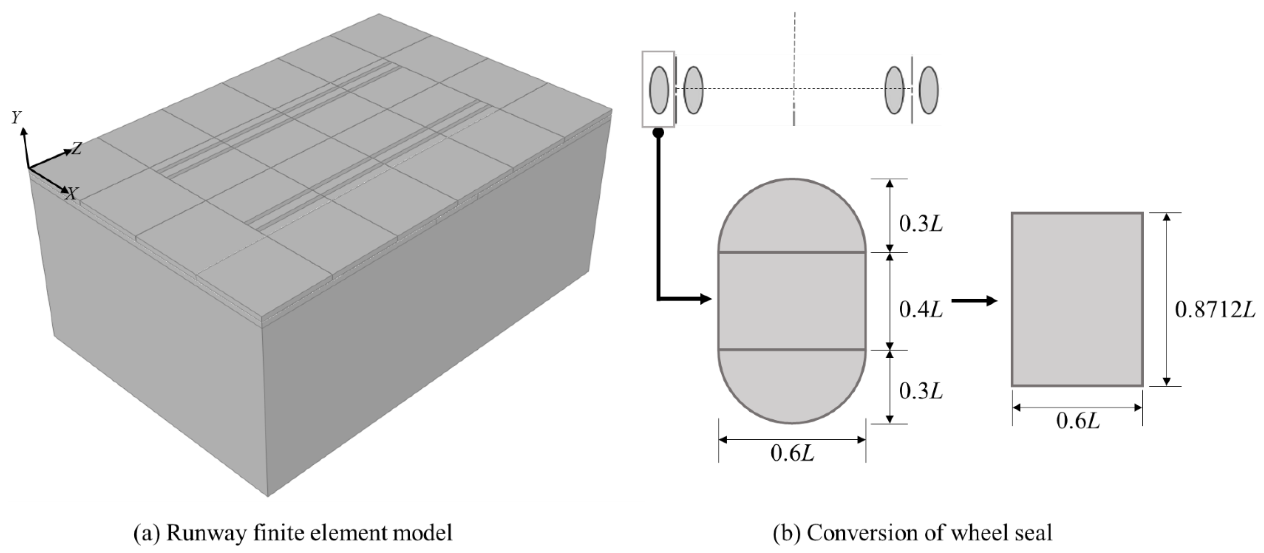
3.1. Runway Structural Parameters and Dynamic Load Application

In this paper, it was necessary to apply a sliding action load to the model. The runway finite element model was 30 m in length and 20 m in width. We simplified the runway structure into the surface, base, and soil layers. The single cement concrete slab size on the surface was 5 m × 5 m × 0.36 m, and there were 24 slabs in total. The base layer thickness was 0.4 m. When the runway finite element model is used for transient dynamic analysis, the thickness of soil base layer should be greater than 13 m to ensure that the results are not affected by constraints [12]. Therefore, the thickness of soil base layer of runway model was set to 13 m. The overall size of the model was 30 m × 20 m × 13.76 m. Dowel bars were set horizontally between cement concrete slabs, and tie bars were set longitudinally. According to the specification found in [32], the number of dowel bars and tie bars at the edge of the board was 17, and the number of tie bars was 8. The diameters of dowel bars and tie bars were 0.035 m and 0.02 m, respectively; the lengths were 0.5 m and 1 m, respectively; the elastic modulus was 21,000 MPa, the Shear modulus was 80,000 MPa, and Poisson’s ratio was 0.3. They interacted with two adjacent slabs by embedding both ends into concrete, and the distance between two adjacent concrete slabs was 1 cm.

Research has shown that, when a pavement structure is subjected to dynamic load, the static elastic modulus cannot be applied well to the dynamic analysis of the structure. The dynamic elastic modulus (DEM) of elasticity is the ratio of stress to strain of an object under dynamic load, which can adequately reflect the vibration characteristics of materials. Thus, the DEM of each layer of the runway was used for subsequent calculations and analyses [42]. The parameters of each structural layer of the runway are shown in

Table 4. Parameters of runway structural layers.

Structural Layer	Modulus of Elasticity E (MPa)	Dynamic Modulus of Elasticity Ed (MPa)	Density ρ (kg∙m3)	Poisson’s Ratio ν	Damping Factor α (s−1)	Damping Factor β (s−1)	Thickness h (m)
Cement concrete top layer	36,000	49,820	2400	0.15	0.1	0.001	0.36
Cement gravel base layer	1500	2692	2000	0.25	0.1	0.002	0.4
Soil base layer	80	242	1800	0.35	1	0.01	13

.

It was assumed that the runway structure was an elastic layer system. Each layer was completely continuous, the tie bound the surface layer and the base layer, and a hole dissected the base layer and the soil base. The direction of aircraft taxiing was the Z-direction, while the direction of perpendicular aircraft taxiing was the X-direction, and the direction of depth along the runway was the Y-direction. The boundary constraints were applied to the model, and the boundaries in the parallel and perpendicular aircraft taxiing directions were set in the X- and Z-directions. The bottom surface of the soil base was formed to be entirely fixed. The finite element model is shown in Figure 6a. It is generally believed that the shape of the wheel print of the aircraft tire in contact with the road surface is a rectangle with a semicircle on both sides. When the moving load was applied to the finite element model for analysis, consideration was given to the convenient mesh division and calculation accuracy. The wheel print was simplified to a rectangle according to the principle of area equivalence, and Figure 6b shows the wheel print conversion process.

The single wheel ground area, A, can be expressed by Equations (23) and (24).

$$A={(0.3L)}^2\pi +0.4L\times 0.6L.$$

(28)

$$A=\frac{F}{p}.$$

(29)

Equation (25) is the formula for calculating load F on a single aircraft wheel.

$$F=\frac{\eta Mg}{n^{\prime }},$$

(30)

where L is the wheel print conversion factor, p is the aircraft tire pressure (Pa), η represents the weight distribution coefficient of the main landing gear, and $n^{\prime }$ is the number of main landing gear tires.

Using Equation (23), we obtained $L=\sqrt{A/0.5227}$. According to Figure 6b, A = 0.6L·b, and vertical side length b = 0.8712L after conversion to a rectangle. In this paper, we selected the landing gear of the Airbus A320 passenger aircraft, which is a single-axle dual wheel. The corresponding tire pressure was 1.38 MPa at a single wheel static load F of 175.536 kPa [34], and the rectangular wheel print area A of the aircraft after conversion was obtained as 0.1272 m², with a length of 0.424 m and a width of 0.3 m. Assuming that the ground contact area of the tire was constant during taxiing, the model surface was divided into zones, and four loading belts were set for the two single-axle double wheels. We used the method in Section 2.2 to generate the dynamic load, where the taxiing speed was set to 20 m/s, and the IRI was set to 5. Then, the code of loading load was written in the DLOAD subroutine, and the generated taxiing dynamic load was applied to the divided load zone area.

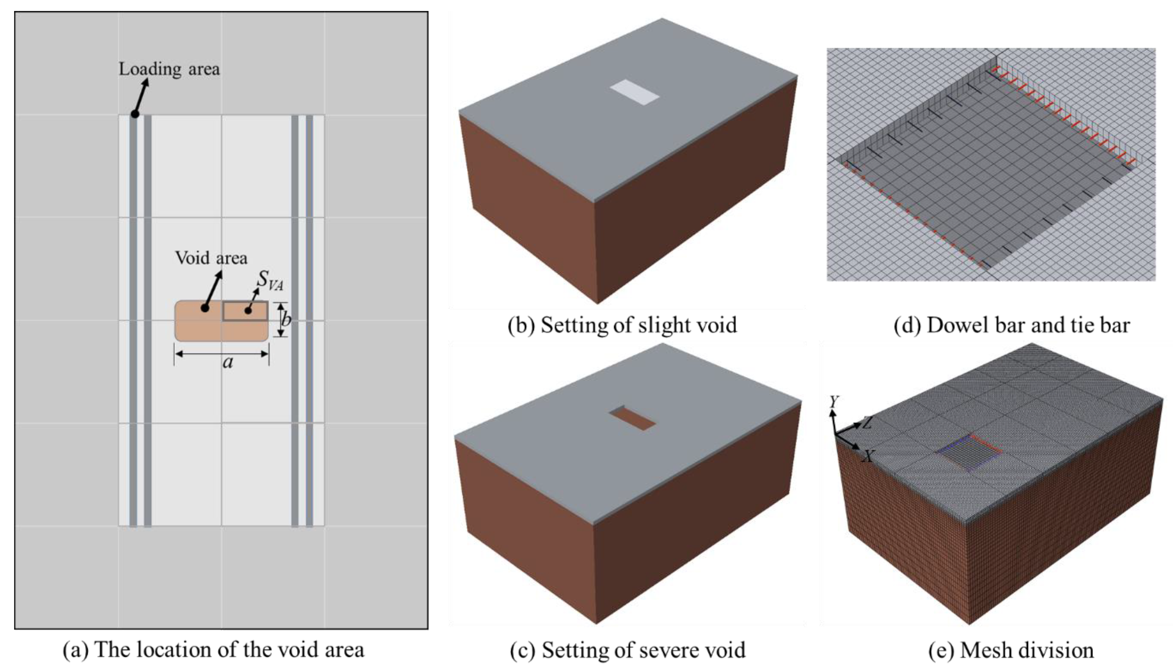
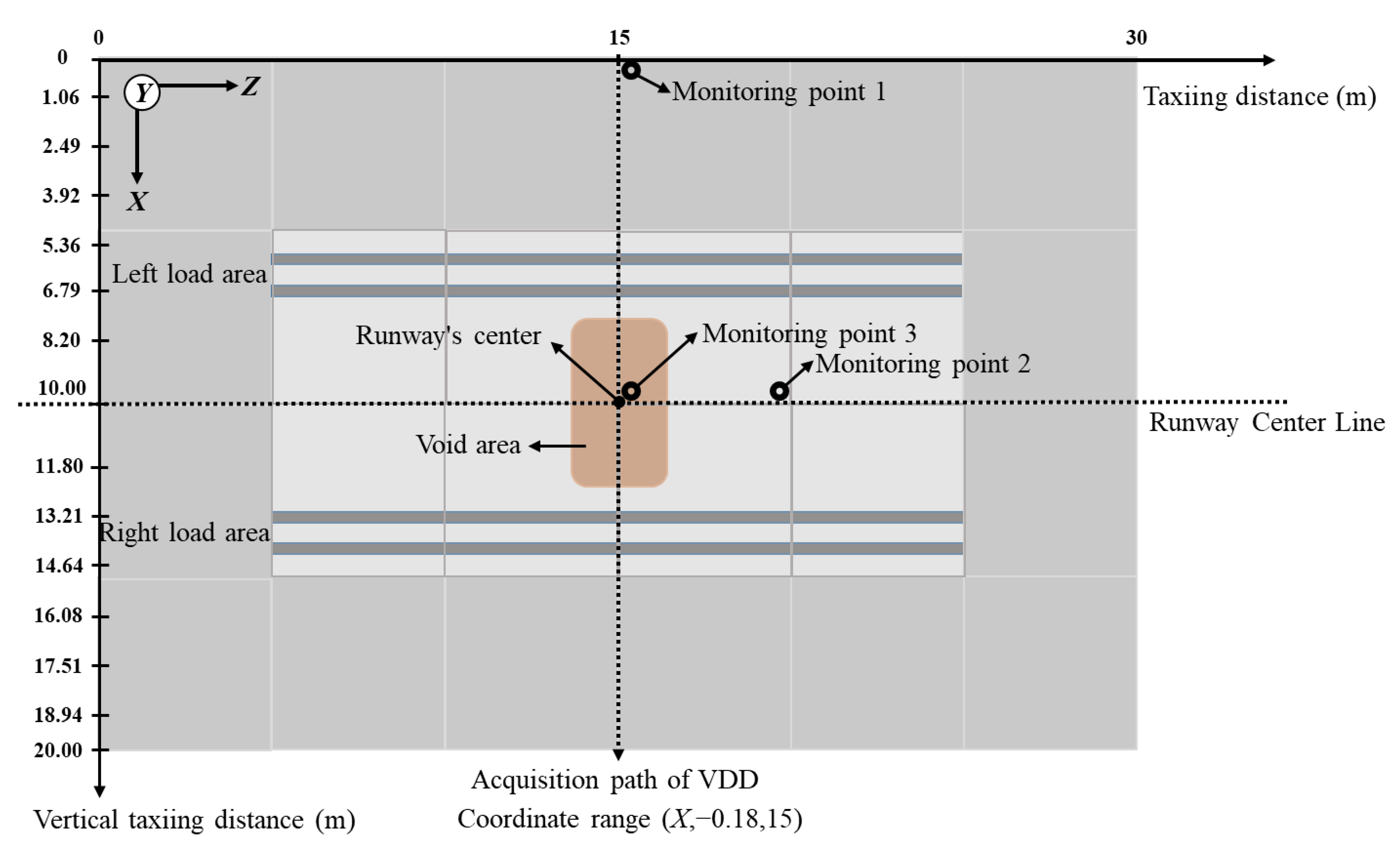
3.2. Void Settings and Mesh Division

In a previous airport runway detection, it was found that the void position mainly occurs at the edge or corner of the concrete slab [43]. The research study showed that, before the pavement slab is completely separated from the base layer, in most cases, the base layer in the void area only loses some fine aggregate, which still has a certain supporting effect on the pavement slab. The response modulus of the base layer is only reduced compared with that without void base layer [44], which is a slight void. After the pavement is separated from the base layer, it becomes a serious void. This paper analyzes and discusses the situations presenting a slight void and a serious void.

Considering the actual situation of the void, it is also necessary to ensure that the mesh division between void and no-void models is consistent to facilitate postprocessing analysis. When establishing the void model in the finite element model, the void location was set in the center of the model, as shown in Figure 7a, located at the edges and corners of the four slabs. In the case of a slight void, the initial dimension of the void area was 5 m in length a and 2.4 m in width b. S_VA is the corner void area of a single board, which remained unchanged at 3.00 m². When there is a slight void, in [44], the degree of the void was reflected by reducing the reaction modulus of the base layer under the slab. In this article, the difference in the pavement void degree was realized by reducing the DEM at the base layer, and ξ represents the reduction coefficient (RC) of the DEM at the base layer in the void area, with the reduced DEM at the base layer being equal to ξ multiplied by the original DEM at the base layer (E_d). The values of ξ were 0.75, 0.5, 0.25, 0.1, 0.01, 0.001, and 0.0001, indicating different degrees of void. ξ equal to 1 indicated a healthy pavement structure. The setting of a slight void is shown in Figure 7b. For the case of a severe void, we deleted the corresponding base area and set the void size a to 5 m, b to 0.6 m, 1.2 m, 1.8 m, 2.4 m, 3.0 m, and 3.6 m, and the corresponding S_VA to 0 m², 0.75 m², 1.50 m², 2.25 m², 3.00 m², 3.75 m², and 4.5 m², respectively. The runway finite element models were established by taking ξ and S_VA as variables.

A reasonable mesh division can reduce the usage of computational resources while ensuring computational accuracy. In the response analysis of the pavement, there are two or more layers of meshes on the surface layer thickness, which can meet the calculation requirements [45]. The mesh size of the runway model surface layer was 0.18 m × 0.18 m × 0.18 m. In order to facilitate void setting and data extraction, the mesh size of the base layer was slightly larger than that of the surface layer, with the size of 0.3 m × 0.3 m × 0.2 m. The length and width of the soil base meshes are consistent with the base layer; referring to the method in [46], the thickness was gradually increased downward from 0.2 m to 1 m to reduce the amount of calculation. The element type used was C3D8R. The C3D8R unit is a reduced integration for eight-node solid elements with three translational degrees of freedom per node [47]. It is suitable for finite element analysis of road structure model [48]. The dowel bar and tie bar are shown in Figure 7d, and a two-node linear beam unit B31 was adopted. The mesh division of the overall runway model is shown in Figure 7e.

Below, we present the analysis and processing of the runway structure’s vertical dynamic displacement response and vibration acceleration signals under different void conditions when the aircraft taxied on the runway. According to the research requirements, seven points were taken from the runway center to both sides to extract the VDD of the pavement slab in the time domain. We set the acquisition path of the VDD, which passed through the runway center and was perpendicular to the centerline of the runway. The path had a depth of 0.18 m and was located in the middle of the surface layer; it was used to extract the VDD of the runway structure when the aircraft tire acted directly above the acquisition path. Simultaneously, monitor points (MPs) 1, 2, and 3 of the vibration acceleration signals were set on the runway surface layer, which was used to extract the pavement slabs’ vertical acceleration response signals under different void conditions. The specific acquisition path of the VDD and the arrangement of acceleration signal monitor points are shown in Figure 8.

4. Analysis of Results and Discussion

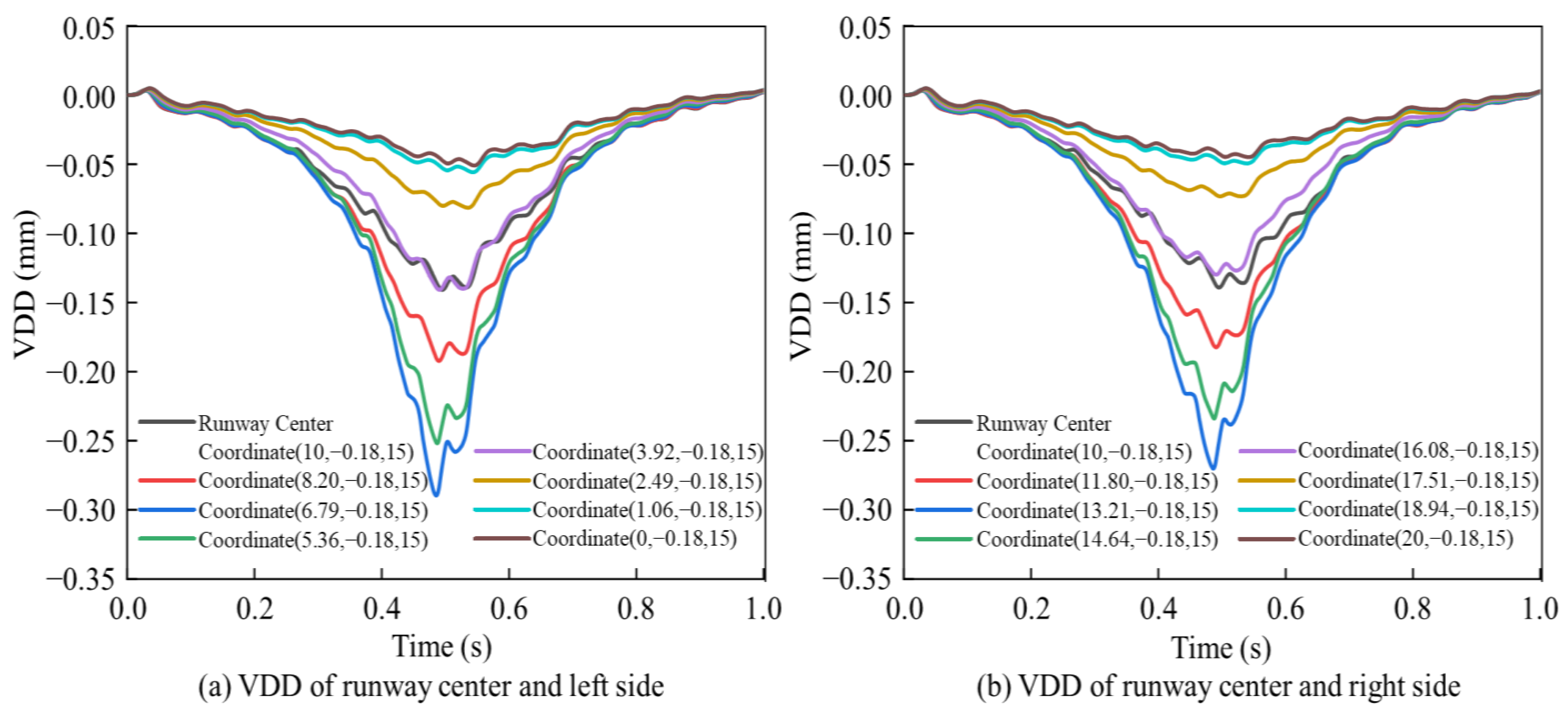
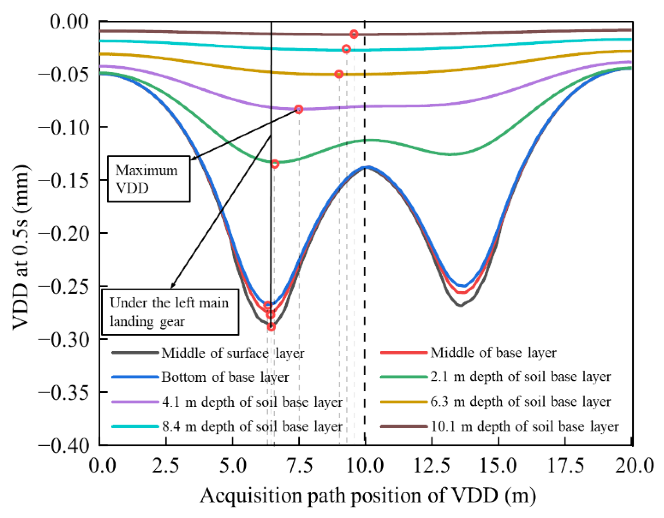
4.1. Calculation Results of VDD with No Void

The above calculations were completed in ABAQUS finite element software. The load transfer coefficient was calculated to be above 95% by the displacement at the corresponding position of the adjacent panels, which proved that the rigid pavement model had good load transfer performance. When there was no void in the pavement, the time-domain VDD of the collected pavement was calculated as shown in Figure 9a,b using the acquisition points on the acquisition path of the VDD. As the calculation model is a four-degrees-of-freedom, double-main-landing-gear model, the rollover stiffness was considered in the dynamic load calculation. Therefore, the VDDs in the left and correct symmetrical positions on the runway centerline were different, but the VDD trends were consistent with the changes in position and time. At 0.5 s, the main landing gear was located directly above the acquisition path, and the VDDs in different positions were at their maximum values. The smallest VDDs values were at 10 m on the left and right sides of the runway center, 0.050 mm and 0.044 mm, respectively, while 3.21 m to the left and right sides of the runway center was under the inner tire of the main landing gear, with the largest VDD values of 0.290 mm and 0.270 mm, respectively. The peak value of the time-domain VDD in the runway center was 0.141 mm, similar to the peak value of the time-domain VDD at 6.08 m on both sides.

The acquisition path of the VDD was offset to the middle and bottom of the base layer along the negative direction of the y-axis, and the soil base layer depths were 2.1 m, 4.1 m, 6.3 m, 8.4 m, and 10.1 m. There were eight acquisition paths of the VDD with different depths. Figure 10 depicts the VDD results on the eight paths at the 0.5 s moment. The VDDs of the surface and base layers increased first and then decreased from the runway center to both sides, forming an obvious “W” shape with the peaks located directly below the left and right main landing gears. The left main landing gear was currently more loaded, and the VDD at the bottom of the base layer was 0.267 mm, which was only 7% less than the VDD in the middle of the surface layer of 0.287 mm. The reduction rates of the soil base layer were approximately 53.6%, 72.1%, 83.3%, 91%, and 96%at the depths of 2.1 m, 4.1 m, 6.3 m, 8.4 m, and 10.1 m, respectively, compared with the VDD of 0.267 mm in the middle of the surface layer. The soil base layer’s VDD increased with depth and then decreased. We marked the VDD peak on the left side of the runway center of the eight paths. The maximum VDD of each left path was shifted to the runway center as the acquisition path depth increased, and the shifting amplitude in the interval from the surface layer to the soil base at a depth of 2.1 m was small, about 0.2 m. The maximum value of VDD was about 3 m in the soil base depth range from 2.1 m to 10.1 m, which was close to the runway center. Below the runway center, the VDD of the surface layer and the base layer barely changed. The VDD of the soil base changed uniformly along the runway depth direction. When the acquisition path depth exceeded 6.3 m, the maximum value of VDD decreased noticeably.

Section 4.2 and Section 4.3 investigate the runway surface layer’s VDD response and vibration signal during aircraft taxiing on runways under different runway pavement void conditions.

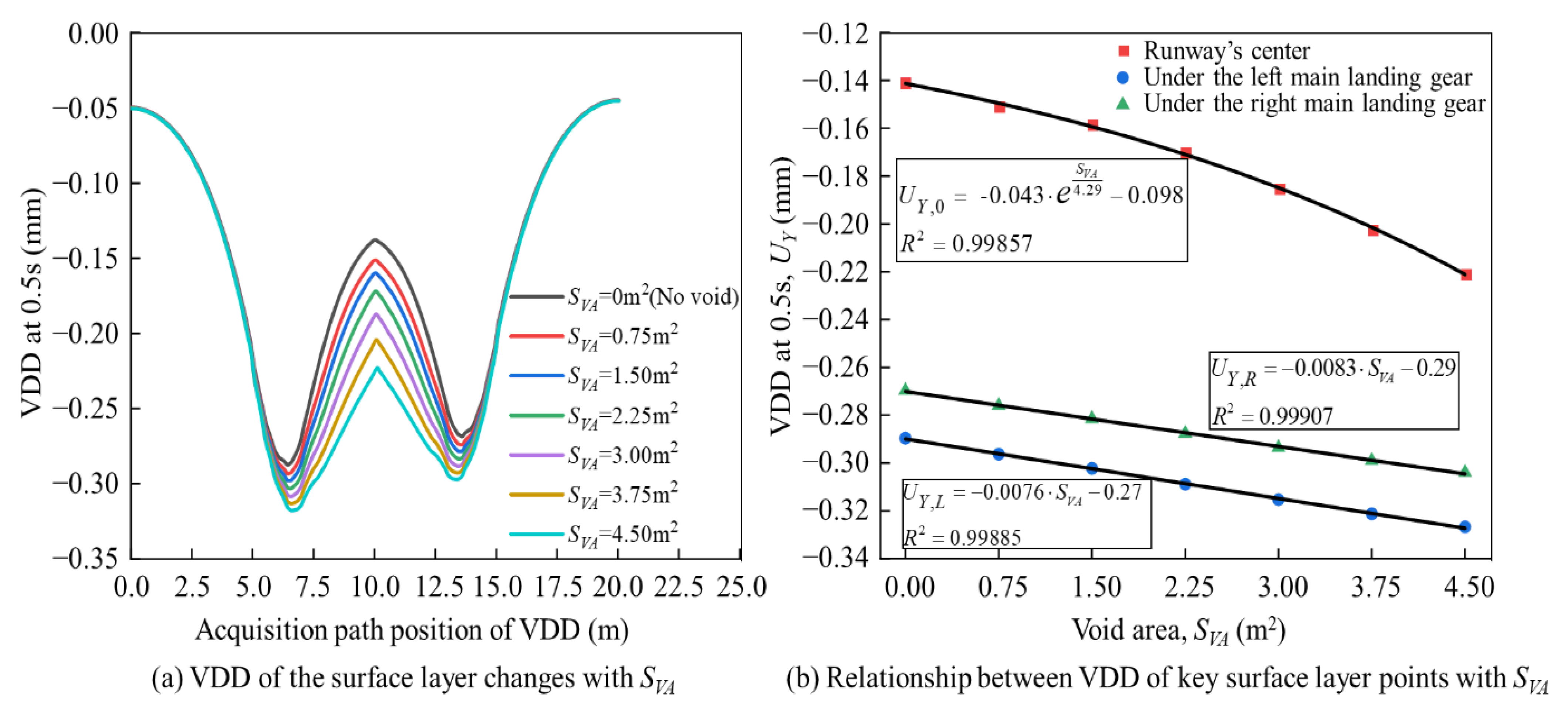
4.2. Analysis of Dynamic Displacement Calculation Results with Void

When the main landing gear was located directly above the acquisition path of the VDD, the VDD results for the middle of the surface layer were extracted from several groups of models with different degrees of the void.

For the slight void state, the change in the dynamic displacement of the surface layer with the decrease in ξ is shown in Figure 11a. With the decrease in ξ, the instantaneous VDD of the pavement increased on the whole, and the variation in the VDD on the VDD acquisition path gradually became larger from both sides to the runway center. ξ varied from 1 to 0.1, and the variation in the VDD of the road surface was not obvious, while the five curves almost overlapped, and the VDD in the runway center was about 0.138 mm. When ξ was 0.01, 0.001, or 0.0001, the VDD in the runway center was 0.151 mm, 0.164 mm, or 0.166 mm, respectively. The difference between the curves was minimal when ξ was 0.001 or 0.0001, indicating that the change in the VDD of the pavement was not noticeable when the modulus of the void area was less than 2.692 MPa. Figure 11b shows the results of the regression analysis of the VDD in the middle of the surface layer with ξ, where U_Y,0, U_Y,L, and U_Y,R represent the VDDs in the middle of the surface layer in the runway center and under the left and right main landing gears. U_Y,0 showed a negative exponential variation law with ξ, with a coefficient of determination of 0.99932. U_Y,L, and U_Y,R showed a logarithmic variation relationship with ξ, with coefficients of determination of 0.9853 and 0.9855, respectively.

When the pavement slab had a serious void, with the increase in S_VA, the VDD of the surface layer changed as shown in Figure 12a. With the increase in S_VA, the VDD under the two main landing gears had a relatively obvious increase. The VDD in the runway center was the most obvious distinction. The VDD of the surface layer was 0.139 mm when it had no void; compared with that when S_VA assumed values of 0 m², 0.75 m², 1.50 m², 2.25 m², 3.00 m², 3.75 m², and 4.5 m², the increases were 10.1%, 16.5%, 25.9%, 37.4%, 50.4%, and 64.7%, respectively. Figure 12b shows the regression analysis results of the VDD in the middle of the surface layer with S_VA, where U_Y,0, U_Y,L, and U_Y,R represent the VDD in the middle of the surface layer in the runway center and under the left and right main landing gears. It was obtained that U_Y,0, and S_VA showed an exponential variation law with a coefficient of determination of 0.99857. U_Y,L, and U_Y,R showed a linear variation relationship with ξ with the coefficients of determination of 0.99907 and 0.99885, respectively.

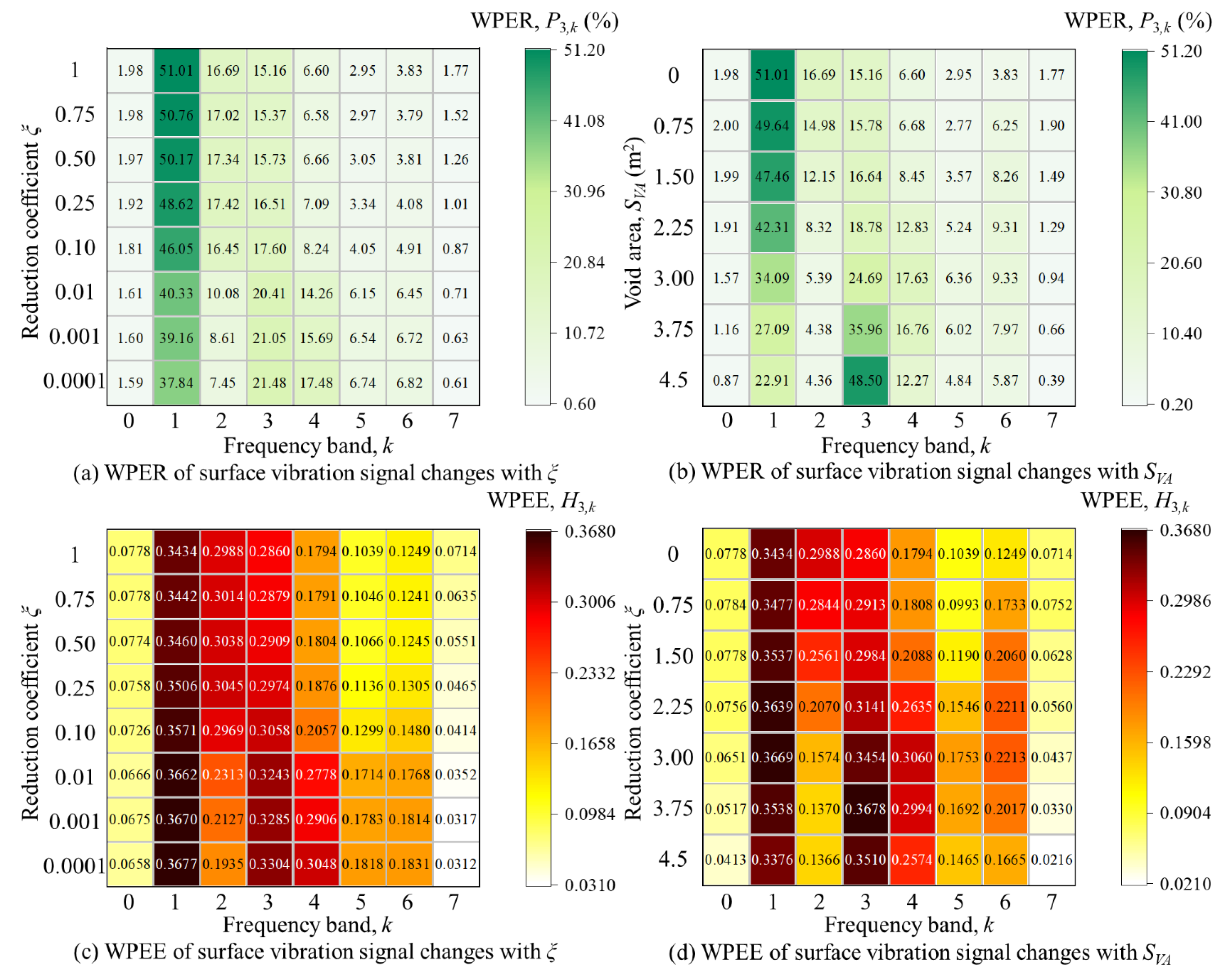
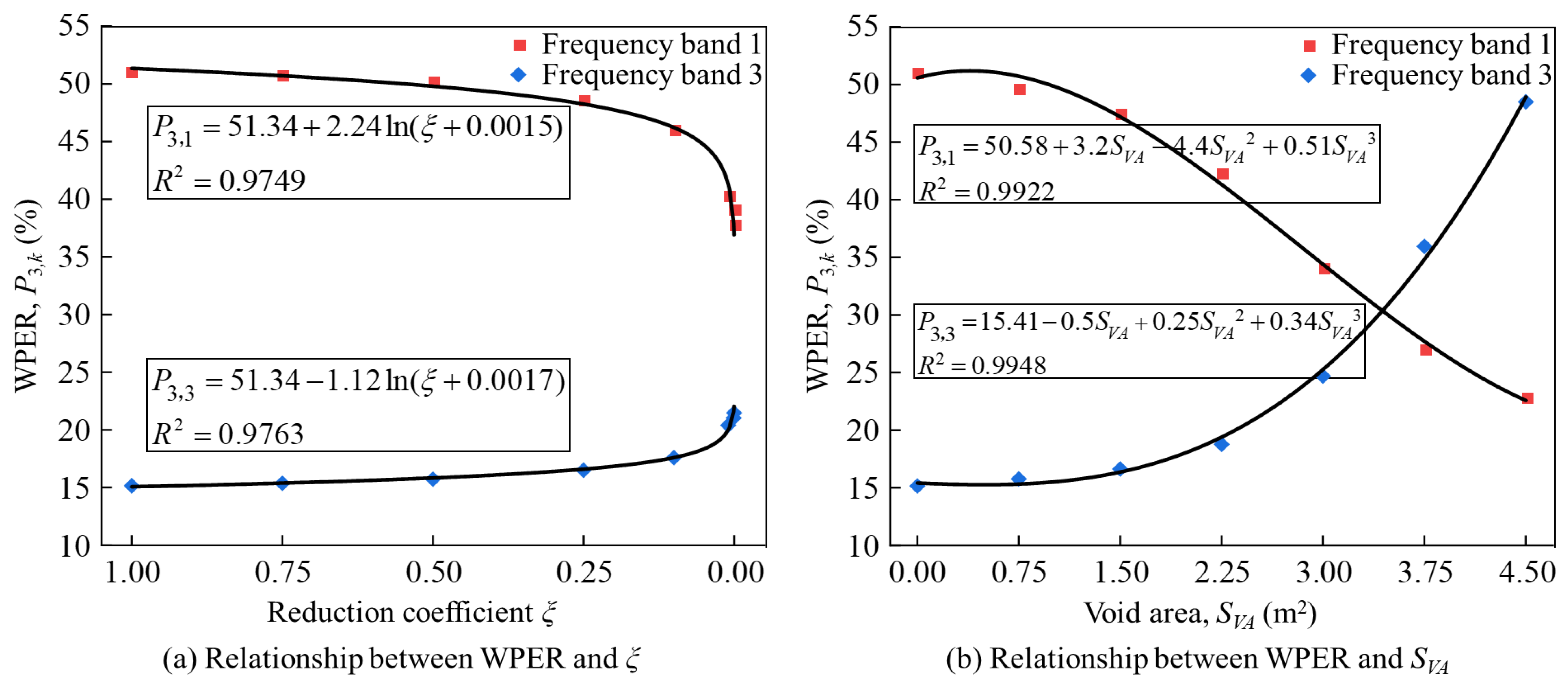
4.3. Analysis of Vibration Acceleration Response Signal of Road Panel

The vibration acceleration signals of various sampling points were extracted from two types and 14 groups of models. According to the calculation, when the wavelet order was 4, the corresponding LP norm entropy was small. As a result, the db4 wavelet base was used to decompose the vibration acceleration signals into three layers, with a bandwidth of 12.5 Hz corresponding to eight uniform frequency bands. The energy distribution of different frequency bands was obtained using the energy characteristic calculation formula of the wavelet packet. Figure 13, Figure 14 and Figure 15 depict the energy distribution law of each frequency band of vibration signals measured by monitor points 1, 2, and 3 for different void states of runway pavement when the aircraft taxiing dynamic load acted. Among them are the WPER of each frequency band of the signals of the three monitor points and the WPEE of the signals of monitor point 3. In general, the vibration acceleration signal energy of the runway surface was primarily concentrated in frequency bands 0–4 or the range of 0–62.5 Hz, but the distribution of the vibration acceleration signal energy at different monitor points varied.

The calculation results of the energy characteristics of 14 groups of wavelet packets for mild and severe voids were analyzed. At monitor point 1, it can be seen from Figure 13a,b that the cumulative WPER of frequency bands 0–3 accounted for more than 90%, while the cumulative WPER of frequency bands 4–7 accounted for less than 10%. At monitor point 2, Figure 14a,b shows that the cumulative WPER of frequency bands 0–3 was greater than 95%, while the cumulative WPER of frequency bands 4–7 was less than 5%. The vibration signal energy at monitor points 1 and 2 was mostly distributed in the 0–50 Hz frequency range.

When the void was slight, the degree of void increased with the decrease in ξ. In eight groups of models, ξ decreased from 1 to 0.0001. From Figure 13a,b, it can be seen that the maximum variation in the WPER of each frequency band of the signal at monitor point 1 was less than 2%. The maximum variation in the WPER of each signal’s frequency band at monitor point 2 was less than 1%. In the case of the severe void, void area S_VA increased from 0 m² to 4.5 m² in seven groups of models. From Figure 14a,b, it can be seen that the maximum variation in the WPER of each frequency band of the signal at monitor point 1 was less than 3%. The maximum variation in the WPER of each signal’s frequency band at Monitor Point 2 was less than 1%.

The WPEE calculation results of the signals at Monitor Points 1 and 2 were analyzed. The same group of signals changed with the frequency band, and its corresponding WPEE change was consistent with the WPER change trend. As different groups of signals changed with ξ and SVA, the WPEE of each frequency band changed very little, and the maximum change was less than 0.01.

When the DEM and void area of the base in the void area changed, the changes in the WPER and WPEE of each frequency band at Monitor Points 1 and 2 were not obvious; thus, they were not sensitive to the changes in pavement void damage. Therefore, in practical engineering, it was found that it is difficult to arrange the acceleration signals collected by sensors at monitor points 1 and 2 to analyze and extract the energy distribution characteristics of wavelet packets and judge the degree and area of hollowing.

For monitor point 3, which was located in the corner of the pavement slabs in the void area, compared with monitor points 1 and 2, from Figure 15a,b, it can be seen that the vibration acceleration signal energy was concentrated in bands 1–4, i.e., 12.5–62.5 Hz, with the WPERs of frequency bands 1 and 3 being relatively large and the sum of the WPERs of each group of frequency bands 1 and 3 all reaching more than 65% of the total energy. From Figure 15c,d, it can be seen that the WPEEs were larger in frequency bands 1–4, and the WPEEs were smaller in frequency band 0, as well as frequency bands 5–7. This indicates that the signal energy and frequency distribution were more scattered in the 12.5–62.5 Hz range, and the signal energy and frequency distribution were relatively stable in the range of 0–12.5 Hz and the high-frequency band (transverse analysis).

After analyzing the wavelet packet energy of the signal at monitor point 3, the WPERs of frequency bands 1 and 3 and the WPEEs of frequency bands 1–3 were more thoroughly studied.

When the pavement was slightly void, ξ decreased from 1 to 0.0001. According to Figure 15a, the WPER of frequency band 1 decreased monotonically from 51.01% to 37.84%, with a variation of 13.17%. The WPER of frequency band 3 increased monotonically from 15.16% to 21.48%, with a variation of 6.32%. According to Figure 15c, the WPEE of frequency band 1 increased monotonically from 0.3434 to 0.3677, with a variation of 0.0243, and that of frequency band 3 increased monotonically from 0.2860 to 0.3304, with a variation of 0.0444.

When the pavement was seriously void, S_VA increased from 0 m² to 4.75 m². From Figure 15b, the WPER of frequency band 1 decreased monotonically from 51.01% to 22.91%, with a variation of 28.1%, whereas the WPER of frequency band 3 increased monotonically from 15.16% to 48.50%, with a variation of 33.34%. From Figure 15d, When S_VA increased from 0 m² to 4.75 m², the WPEE in frequency band 2 decreased monotonically from 0.2988 to 0.1366, with a variation of 0.1622, whereas the WPEEs of frequency bands 1 and 3 did not change monotonically, showing a monotonic increase at first and then a monotonic decrease, reaching the maximum at S_VA values of 3 m² and 3.75 m², respectively. This demonstrates that, as S_VA increased from 0 to 3.75 m², the degree of the dispersion of the vibration signal energy distribution in frequency bands 1 and 3 gradually increased. The vibration signal energy distribution tended to be stable as SVA increased from 3.75 m².

For the signals collected at monitor point 3, the results of the wavelet packet energy analysis were analyzed. P_3,1 and P_3,3 represent the energy ratios of frequency bands 1 and 3. A regression analysis was performed on them with 1 and 2, respectively. The regression results are shown in Figure 16a,b. P_3,1 and P_3,3 were logarithmic with ξ, and the coefficients of determination were 0.9749 and 0.9763, respectively. P_3,1 and P_3,3 had a cubic curve relation with S_VA, and the coefficients of determination were 0.9922 and 0.9948, respectively.

Figure 17 shows the change in the WPEEs of frequency bands 1–4 of the signal at monitor point 3 considering different void states. Combined with the comprehensive analyses of Figure 16a,b and Figure 17a,b, it can be seen that when the vibration acceleration monitor point was located at the corner of the plate, after the wavelet packet energy analysis of the collected signal, the DEM of the base layer in the void area decreased, and the energy ratio and energy entropy of the first and third frequency bands had obvious gradient changes, with the changing trend being monotonous. In the case of the severe void of the pavement slab, with the increase in the void area, the energy ratios of frequency bands 1 and 3 and the energy entropies of the wavelet packet of frequency band 2 changed more obviously, showing a monotonous trend.

In actual engineering, the void of pavement slabs mostly occurs at the corners and edges of slabs. Therefore, through wavelet packet energy analysis, the energy ratios and energy entropies of frequency bands 1 and 3 could be obtained from the vibration signal of the slab angle, which can judge the damage degree of runway pavement slab when it is slightly void. If the pavement slab is severely void, the vibration signal of the slab corner can be analyzed by analyzing the wavelet packet energy, and the WPERs of frequency band 1 and frequency band 3 and the WPEEs of frequency band 2 can be used to identify the area of the slab corner hollowing out.

5. Conclusions

This paper investigated the interaction between the aircraft and the runway during taxiing and developed a simulation model of the vibration system. In addition, the dynamic load of aircraft taxiing was calculated on the pavement, and the vertical dynamic displacement (VDD) response and the variation law of the runway under the action of a moving load were investigated thoroughly. Simultaneously, the energy distribution characteristics of the wavelet packets of acceleration signals in various positions of the pavement slabs were extracted, and the relationship between the energy distribution of specific wavelet packets and void status was discussed. The findings are summarized below.

(1)

Using the simplified 4-DOF aircraft-runway coupled vibration model, runway pavement roughness was used as the load excitation source to calculate the dynamic load of the aircraft taxiing quickly and accurately, applying the state space method.

(2)

When the aircraft taxied on the normal runway structure, the peak VDD of the base layer decreased by only 7% compared with that of the runway surface layer. When the depth of the soil foundation was 2.1 m, the peak value of the VDD decreased by 53% compared with that of the surface layer. When the depth of the soil foundation was greater than 8.4 m, the change in VDD was not obvious. With the increase in depth, the position of the peak VDD gradually shifted to the runway center. In the depth range of 8.1–10.1 m of soil foundation, the position of the peak VDD shifted to the runway center by 3.2 m.

(3)

When the pavement was slightly void, the VDD (U_Y,0) calculated for the runway central point of the surface layer did not change obviously with the decrease in modulus reduction coefficient ξ in the hollowed area in the range of 1–0.1, but with the decrease in ξ from 0.1, U_Y,0 increased sharply. On the whole, U_Y,0 had a negative exponential relationship with ξ. The vertical displacements of the lower surfaces of the left and right main landing gears (U_Y,L, U_Y,R) were logarithmic with ξ. When there was a severe void, U_Y,0 decreased with the increase in void area SVA, and the overall relationship was exponential. U_Y,L, U_Y,R decreased linearly with the increase in S_VA. On the whole, U_R,0 could better reflect the vacancy situation.

(4)

When the aircraft taxiing load acted on the rigid runway, the angular vibration response signal of the road panel caused by it was used. The wavelet packet energy characteristics of the signal, the ratio of the wavelet packet energy in the low-frequency band, and the entropy of the wavelet packet energy could be extracted, which could be used as the eigenvalues to identify the void condition of the runway pavement.

According to the above research results, it can be seen that the dynamic displacement of the rigid runway concrete slab along the runway width direction and the wavelet packet energy ratio and wavelet packet energy entropy could be obtained from the acceleration signal of slab corner under the aircraft load. All of them could be used to reflect the supporting condition or void area of the pavement slab by the base layer. Therefore, embedded displacement sensors can be arranged at the lateral edge of the pavement slab, and embedded acceleration sensors can be arranged at the corner of the slab. In this way, it can be effectively sensed whether the runway panel has a void, as well as its degree, by using the taxiing effect of the aircraft without stopping the airport. This provides a new idea and method for the identification of airport runway slab voids and provides a certain reference value for the implementation of runway health monitoring.

References

1. Civil Aviation Administration of China. CAAC Issues 2021 Statistical Bulletin of Civil Airport Development in China; Civil Aviation Administration of China: Beijing, China, 2022. [Google Scholar]
2. Birkhoff, J.W.; McCullough, B.F. Detection of Voids Underneath Continuously Reinforced Concrete Pavements; University of Texas at Austin, Center for Highway Research: Austin, TX, USA, 1979. [Google Scholar]
3. Yang, D.; Wang, Z. Analysis of measured dynamic response of airport runway under Boeing 777 loading. J. Tongji Univ. Nat. Sci. 2014, 42, 1550–1556. [Google Scholar]
4. Brill, D.R.; Flynn, R.M.; Pecht, F. FAA Rigid Pavement Instrumentation at Atlanta Hartsfield-Jackson International Airport. In 2007 Worldwide Airport Technology Transfer Conference; Federal Aviation Administration American, Association of Airport Executives: Atlantic City, NJ, USA, 2007. [Google Scholar]
5. Zhao, H.; Wu, C.; Wang, X.; Zheng, Y. Pavement condition monitoring system at shanghai pudong international airport. In Pavement Materials, Structures, and Performance; Geotechnical Special Publication: Boston, MA, USA, 2014; pp. 283–295. [Google Scholar]
6. Singh, A.; Cook, K. Analysis of Runway Pavement Distress Using Embedded Instrumentation. In Proceedings of the ASCE Construction Congress, San Juan, Puerto Rico, 2–4 June 2016. [Google Scholar]
7. Park, H.W.; Kim, D.H.; Shim, C.S.; Jeong, J.H. Behavior of Airport Concrete Pavement Slabs Exposed to Environmental Loadings. Appl. Sci. 2020, 10, 2618. [Google Scholar] [CrossRef] [Green Version]
8. Gungor, O.E.; Al-Qadi, I.L.; Garg, N. Pavement Data Analytics for Collected Sensor Data; United States, Department of Transportation, Federal Aviation Administration, William J. Hughes Technical Center: Egg Harbor Township, NJ, USA, 2021. [Google Scholar]
9. Liu, S.; Ling, J.; Tian, Y.; Hou, T.; Zhao, X. Random Vibration Analysis of a Coupled Aircraft/Runway Modeled System for Runway Evaluation. Sustainability 2022, 14, 2815. [Google Scholar] [CrossRef]
10. Taheri, M.R.; Zaman, M.M.; Alvappillai, A. Dynamic response of concrete pavements to moving aircraft. Appl. Math. Model. 1990, 14, 562–575. [Google Scholar] [CrossRef]
11. Shafabakhsh, G.; Kashi, E.; Tahani, M. Analysis of runway pavement response under aircraft moving load by FEM. J. Eng. Des. Technol. 2018, 16, 233–243. [Google Scholar] [CrossRef]
12. Dong, Q.; Wang, J.H.; Zhang, X.M.; Wang, H.; Zhao, J.N. Dynamic response analysis of airport pavements during aircraft taxiing for evaluating pavement bearing capacity. J. Zhejiang Univ.-Sci. A 2021, 22, 736–750. [Google Scholar] [CrossRef]
13. Yi-Qiu, T.; Yong-Kang, F.; Yun-Liang, L.; Chi, Z. Responses of snow-melting airfield rigid pavement under aircraft loads and temperature loads and their coupling effects. Transp. Geotech. 2018, 14, 107–116. [Google Scholar] [CrossRef]
14. Fu, Y.K.; Li, Y.L.; Tan, Y.Q.; Zhang, C. Dynamic response analyses of snow-melting airport rigid pavement under different types of moving loads. Road Mater. Pavement Des. 2019, 20, 943–963. [Google Scholar] [CrossRef]
15. Wu, Y.; Liu, T.; Zhi, H.; Chen, B.; Zheng, Z.; Fang, H.; Yang, K. Experimental study on detection of void in concrete pavement slab by FWD. IOP Conf. Ser. Earth Environ. Sci. 2020, 508, 012080. [Google Scholar] [CrossRef]
16. Su, J.; Zhang, W.; Xiang, H.; Guo, X. Application and Analysis of Ground Penetrating Radar in Non-destructive Testing and Evaluation of Civil Airport Runway. IOP Conf. Ser. Earth Environ. Sci. 2018, 153, 032011. [Google Scholar] [CrossRef]
17. Xie, J.; Niu, F.; Su, W.; Huang, Y.; Liu, G. Identifying airport runway pavement diseases using complex signal analysis in GPR post-processing. J. Appl. Geophys. 2021, 192, 104396. [Google Scholar] [CrossRef]
18. Zhang, J.; Lu, Y.; Yang, Z.; Zhu, X.; Zheng, T.; Liu, X.; Tian, Y.; Li, W. Recognition of void defects in airport runways using ground-penetrating radar and shallow CNN. Autom. Constr. 2022, 138, 104260. [Google Scholar] [CrossRef]
19. Levenberg, E. Inferring pavement properties using an embedded accelerometer. Int. J. Transp. Sci. Technol. 2012, 1, 229–246. [Google Scholar] [CrossRef] [Green Version]
20. Ye, Z.; Lu, Y.; Wang, L. Investigating the pavement vibration response for roadway service condition evaluation. Adv. Civ. Eng. 2018, 2018, 2714657. [Google Scholar] [CrossRef]
21. Sun, Z.; Chang, C.C. Structural damage assessment based on wavelet packet transform. J. Struct. Eng. 2002, 128, 1354–1361. [Google Scholar] [CrossRef]
22. Law, S.S.; Li, X.Y.; Zhu, X.Q.; Chan, S.L. Structural damage detection from wavelet packet sensitivity. Eng. Struct. 2005, 27, 1339–1348. [Google Scholar] [CrossRef]
23. Su, W.C.; Huang, C.S.; Chen, C.H.; Liu, C.Y.; Huang, H.C.; Le, Q.T. Identifying the modal parameters of a structure from ambient vibration data via the stationary wavelet packet. Comput.-Aided Civ. Infrastruct. Eng. 2014, 29, 738–757. [Google Scholar] [CrossRef]
24. Yu, Y.; Ma, W. A Multi-Excitation Method of Damage Detection in Plate-Like Structure Based on Wavelet Packet Energy. Int. J. Struct. Stab. Dyn. 2022, 22, 2250091. [Google Scholar] [CrossRef]
25. Weng, X.C. Airport Road Surface Testing Technology; Transportation Press Co.: Beijing, China, 2017; pp. 83–96. [Google Scholar]
26. Sun, L. Simulation of Pavement Roughness and IRI Based on Power Spectral Density. Math. Comput. Simul. 2003, 61, 77–88. [Google Scholar] [CrossRef]
27. ISO-8608; Mechanical Vibration—Road Surface Profiles—Reporting of Measured Data. International Organization for Standardization: Geneva, Switzerland, 1995.
28. Sayers, M.W. Guidelines for Conducting and Calibrating Road Roughness Measurements; University of Michigan, Transportation Research Institute: Ann Arbor, MI, USA, 1986. [Google Scholar]
29. Tian, Y.; Liu, S.; Liu, L.; Xiang, P. Optimization of International Roughness Index Model Parameters for Sustainable Runway. Sustainability 2021, 13, 2184. [Google Scholar] [CrossRef]
30. Cheng, G.Y.; Hou, D.W.; Huang, X.D. Research on road surface unevenness limit criteria based on vertical acceleration of aircraft. Vib. Shock. 2017, 36, 166–171. [Google Scholar]
31. Schmid, H. How to Use the FFT and MATLAB’s Pwelch Function for Signal and Noise Simulations and Measurements. FHNW/IME 2012, 2–13. Available online: http://schmid-werren.ch/hanspeter/publications/2012fftnoise.pdf (accessed on 23 April 2022).
32. MHJ 5004-2010; Civil Airport Cement Concrete Road Surface Design Specification. People’s Traffic Publishing House: Beijing, China, 2010.
33. Preumont, A. Vibration Control of Active Structures; Kluwer Academic Publishers: Dordrecht, The Netherlands, 1997; Volume 2. [Google Scholar]
34. Airbus S.A.S. Aircraft Characteristics Airport and Maintenance Planning; Airbus SAS Prancis: Blagnac, France, 2005; Available online: https://www.as.arizona.edu/~gschneid/ECLIPSE_WEB/TSE2015/A320_DOCUMENTS/Airbus-AC-A320-Jun2012.pdf (accessed on 6 December 2021).
35. Ling, J.M.; Liu, S.F.; Yuan, J. Comprehensive analysis of pavement roughness evaluation for airport and road with different roughness excitation. J. Tongji Univ. (Nat. Sci.) 2017, 45, 519–526. [Google Scholar]
36. Zhu, L.; Chen, J.; Yuan, J.; Hao, D. Taxing load analysis of aircraft based on virtual prototype. J. Tongji Univ. Nat. Sci. 2016, 44, 1873–1879. [Google Scholar]
37. Ledbetter, R.H. Pavement Response to Aircraft Dynamic Loads; U.S. Army Engineers Waterways Experiment Station Technical Report S-75-11; U.S. Army Corps of Engineers Waterways Experiment Station: Vicksburg, MS, USA, 1975. [Google Scholar]
38. Chun-Lin, L. A tutorial of the wavelet transform. NTUEE Taiwan 2010, 21, 22. [Google Scholar]
39. Chui, C.K. An Introduction to Wavelets; Academic Press: New York, NY, USA, 1992. [Google Scholar]
40. Learned, R.E.; Willsky, A.S. A wavelet packet approach to transient signal classification. Appl. Comput. Harmon. Anal. 1995, 2, 265–278. [Google Scholar] [CrossRef] [Green Version]
41. Zhou, K.; Lei, D.; He, J.; Zhang, P.; Bai, P.; Zhu, F. Real-time localization of micro-damage in concrete beams using DIC technology and wavelet packet analysis. Cem. Concr. Compos. 2021, 123, 104198. [Google Scholar] [CrossRef]
42. Zeng, S. Research on Pavement Performance Evaluation and Analysis Methods; Central South University: Changsha, China, 2003. (In Chinese) [Google Scholar]
43. Dong, M.; Hayhoe, G.F. Analysis of Falling Weight Deflectometer Tests at Denver International Airport; Federal Aviation Administration: Washington, DC, USA, 2002. [Google Scholar]
44. Tan, Y.; Ling, J.M.; Yuan, J.; Xu, Z. Influence of voids to loading stresses of airport cement concrete pavement. J. Tongji Univ. Nat. Sci. 2010, 38, 552–556. [Google Scholar]
45. Zhou, Z.F.; Ling, J.M.; Yuan, J. 3-D finite element analysis of the load transfer efficiency of joints of airport rigid pavement. China Civ. Eng. J. 2009, 42, 112–118. [Google Scholar]
46. Wu, J.; Liang, J.; Adhikari, S. Dynamic response of concrete pavement structure with asphalt isolating layer under moving loads. J. Traffic Transp. Eng. (Engl. Ed.) 2014, 1, 439–447. [Google Scholar] [CrossRef] [Green Version]
47. Ai, Z.Y.; Xu, C.J.; Zhao, Y.Z.; Liu, C.L.; Ren, G.P. 3D dynamic analysis of a pavement plate resting on a transversely isotropic multilayered foundation due to a moving load. Soil Dyn. Earthq. Eng. 2020, 132, 106077. [Google Scholar] [CrossRef]
48. Chen, X.; Zhu, Y.; Cai, D.; Xu, G.; Dong, T. Investigation on Interface Damage between Cement Concrete Base Plate and Asphalt Concrete Waterproofing Layer under Temperature Load in Ballastless Track. Appl. Sci. 2020, 10, 2654. [Google Scholar] [CrossRef] [Green Version]
Figure 1. Research methods and steps.
Applsci 12 07465 g001
Figure 2. The roughness curve of pavement and the power spectrum density (PSD) of pavement were verified.
Applsci 12 07465 g002
Figure 3. Simplified 4-DOF aircraft runway vibration model.
Applsci 12 07465 g003
Figure 4. Simulation model of aircraft-runway vibrations.
Applsci 12 07465 g004
Figure 5. Dynamic load of aircraft main landing gear.
Applsci 12 07465 g005
Figure 6. Finite element model of runway and loading wheel print.
Applsci 12 07465 g006
Figure 7. Void mode and mesh generation of model.
Applsci 12 07465 g007
Figure 8. Acquisition path of VDD and vibration signal monitor points.
Applsci 12 07465 g008
Figure 9. Multipoint dynamic displacement of surface dynamic displacement acquisition path in the time domain.
Applsci 12 07465 g009
Figure 10. VDDs of different structural layers.
Applsci 12 07465 g010
Figure 11. VDD of pavement in case of slight void.
Applsci 12 07465 g011
Figure 12. VDD of pavement in case of severe void.
Applsci 12 07465 g012
Figure 13. Energy distribution characteristics of vibration signal at monitor point 1.
Applsci 12 07465 g013
Figure 14. Energy distribution characteristics of vibration signal at monitor point 2.
Applsci 12 07465 g014
Figure 15. Energy distribution characteristics of vibration signal at monitor point 3.
Applsci 12 07465 g015
Figure 16. The change in the WPERs of frequency bands 1and 3 of the signal at monitor point 3.
Applsci 12 07465 g016
Figure 17. The change in the WPEEs of frequency bands 1–4 of the signal at monitor point 3.
Applsci 12 07465 g017