Abstract
The measurement of grape sugar content is an important index for classifying grapes based on their quality. Owing to the correlation between grape sugar content and appearance, non-destructive measurements are possible using computer vision and deep learning. This study investigates the quality classification of the Red Globe grape. The number of collected grapes in the range of the 15~16% measure is three times more than in the range of <14% or in the range of the >18% measure. This study presents a framework named feature normalization reweighting regression (FNRR) to address this imbalanced distribution of sugar content of the grape datasets. The experimental results show that the FNRR framework can measure the sugar content of a whole bunch of grapes with high accuracy using typical convolution neural networks and a visual transformer model. Specifically, the visual transformer model achieved the best accuracy with a balanced loss function, with the coefficient of determination R = 0.9599 and the root mean squared error RMSE = 0.3841%. The results show that the effect of the visual transformer model is better than that of the convolutional neural network. The research findings also indicate that the visual transformer model based on the proposed framework can accurately predict the sugar content of grapes, non-destructive evaluation of grape quality, and could provide reference values for grape harvesting.
1. Introduction
The measurement of grape sugar content, and their quality, is the primary activity in packaging, preservation, storage, and transportation. The identification of the sugar content of grapes relates to both grape quality and the determination of storage time before consumption. With the development of the table grape industry towards large-scale and centralized development, an objective and non-destructive testing method is required to monitor the grading of grape quality in the supply chain to meet the needs of large-scale production [1].
1.1. Related Work
Phenotypic characteristics, such as the degree of fruit coloration and concentration, are important indicators for judging table grapes’ maturity and quality [2,3]. Grape color is caused by the accumulation of anthocyanins in the peel. Anthocyanins are a type of water-soluble pigment, and their presence is positively correlated with fruit coloration [2]. Red light irradiation during plant growth increases the degree of fruit coloring, and the sugar content increases accordingly [3]. This demonstrates how the color concentration of grape peel has a positive correlation with sugar content. The correlation coefficients of anthocyanin content and fruit color index of the four grapes “Jingxiu,” “Juxing,” “Fujiminori,” and “Yongyou” were 0.821, 0.946, 0.996, and 0.857, respectively. Additionally, the correlation coefficients of anthocyanins and sugar content were 0.804, 0.953, 0.932, and 0.911, respectively [3]. Visual characteristics of table grapes can reflect the physiological characteristics of a bunch of grapes during the growth process; hence, this provides a research method for predicting the sugar content of grapes using visual features.
Computer vision technology has been widely used in agricultural production as it is fast and non-destructive compared to manual detection [4,5]. Computer vision detection methods are based on grape color and shape, feature fusion, and deep learning. Information on the color channels in the L*a*b color space translated from RGB images was applied to extract color features, which has the potential for apple sugar content prediction [6]. A combination of visible-range image processing, image feature extraction, a hybrid imperialist competitive algorithm, and artificial neural network regression yielded a squared correlation coefficient (R2) on the pH value of 0.843 ± 0.043 on a test set of Thomson navel oranges [7]. Experiments show that color features can determine the internal fruit quality. In [8], an RGB image of oranges was obtained using a camera, and the color, shape, and texture features were extracted from the image and used as the input value for the neural network model that predicted the sugar content and pH value. The results found that neural networks could determine sugar content and pH with high accuracy solely from the appearance of the fruit. A multiple linear regression model of the Red Globe grape’s color features and sugar content was established to classify boxes of Red Globe grapes in [9], where the R2 was 0.84 and the RMSE was 0.82%. The color, shape, and texture characteristics of an orange, taken from an image, were used to predict the sugar content and pH value. The model was able to predict the sugar content and pH value accurately. These methods mentioned above demonstrate the feasibility of using computer vision methods to detect the internal quality of fruits non-destructively.
1.2. Contribution
In this study, we divided the grape dataset into multiple categories based on the imbalanced distribution of the grape’s sugar content. A deep convolutional neural network, transfer learning method, and transformer model are adopted to extract the image features of the grapes from the input data. We then present a computer vision system for non-destructive testing of table grapes. The system was upgraded by optimizing the loss function, which improved the accuracy of the test dataset. The major contributions are as follows:
- (a)
- A feature normalization reweighting regression network (FNRR-Net) is proposed for imbalanced distribution grape datasets, which has a high degree of confidence in predicting the sugar content of grapes.
- (b)
- We group and label the datasets in different sugar content intervals and propose a balanced loss function under the visual transformer model to accommodate the imbalanced grape datasets.
- (c)
- The non-destructive measurement of a grape’s sugar content is efficient, economical, and convenient.
2. Materials and Methods
2.1. Sample Collection
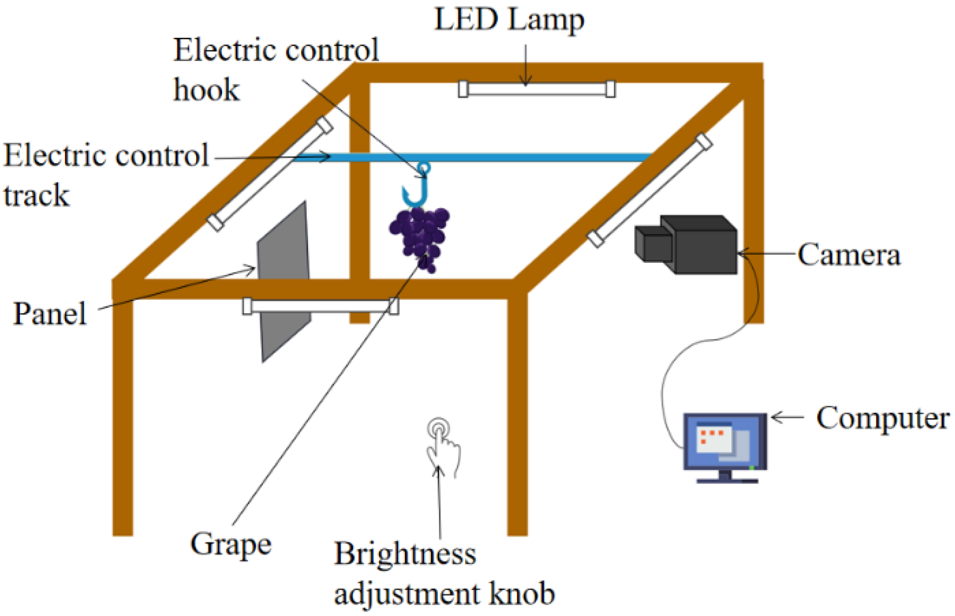
The sample comprised Red Globe grapes harvested from a local market in Wuhan, China. Imitating the industrial inspection process, we designed a grape image acquisition system (Figure 1), consisting of the following components: A panel, an electric control track, an electric control hook, a camera, a brightness adjustment knob, a computer, and four LED lamps. Image acquisition was performed between 9 a.m. and 6 p.m. in the laboratory where the temperature is approximately 25 °C. The panel was used as the background, and the electric control track transported the electric control hook, with grapes attached, to the front of the panel, while the brightness adjustment knob controlled the brightness of the chassis by controlling the lamp. The length of the LED lamp was 30 cm, the power of the LED lamp was 7.9 W, the color temperature was 6500 K when photographing, the electric control track was located in the center of the four led lights, and its vertical distance was 30 cm. The computer used a JAI AD080GE camera to take pictures of the grapes, and the resolution of the obtained images was 1024 × 768 pixels. The distance between the grapes and the camera was 35 cm, and the distance between the grapes and the background plate was 15 cm. The grapes were numbered for imaging and sugar content measuring. A saccharometer is an instrument that measures sugar content, developed according to the principle of optical refraction; it is commonly used to measure the sugar content of fruit juice. This study used a VBS2T/ATC saccharometer, which had a measurement precision (Brix%) of 0.2. In total, 228 pictures were collected using the image acquisition system; 205 were used to train the model, and the model was tested on the remaining 23.

Figure 1.
Grape image acquisition system.
2.2. Image Pre-Processing
2.2.1. Image Extraction
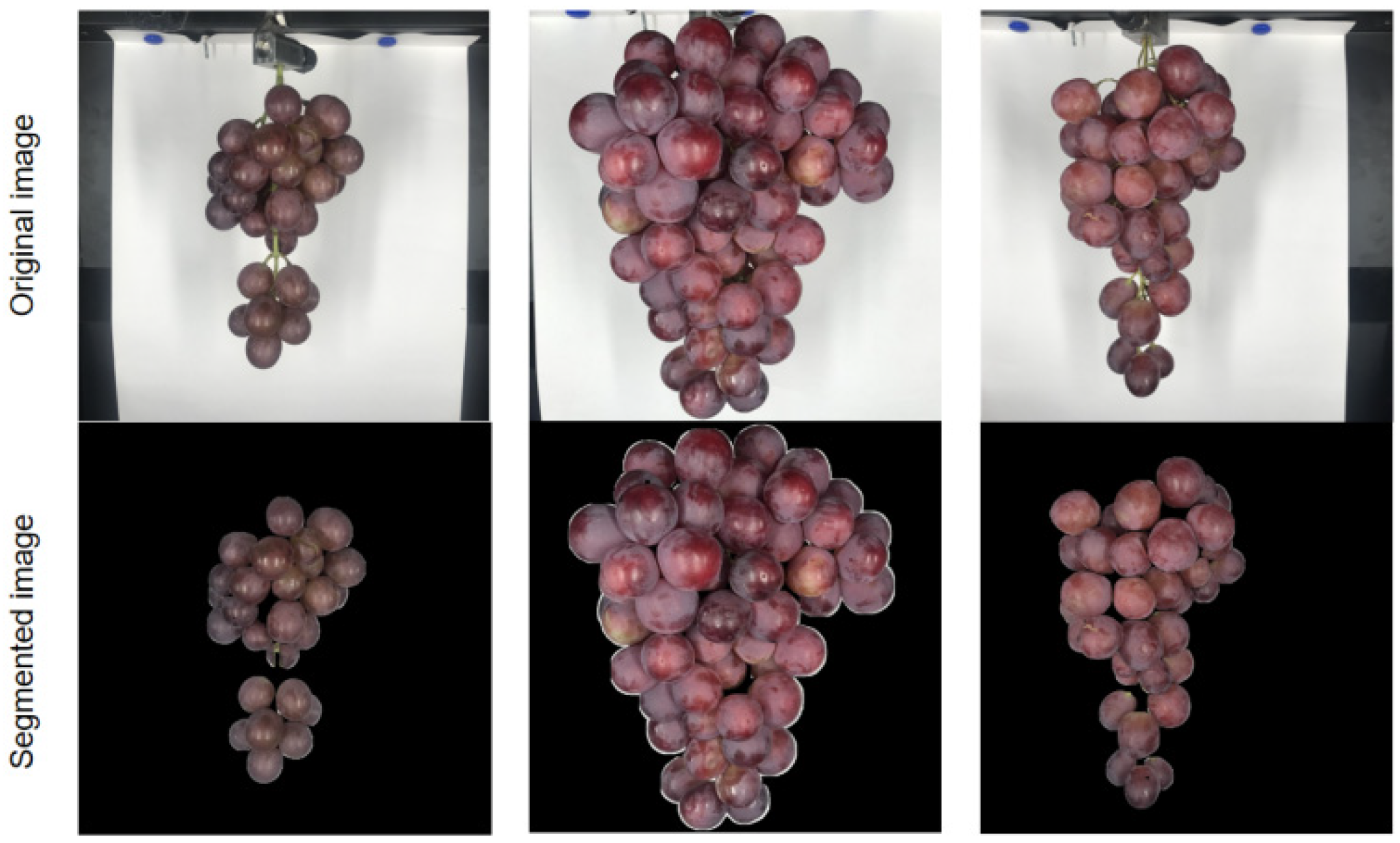
Foreground segmentation was performed to better extract the features from the grape images (shown in Figure 2). U-Net [10], a deep segmentation model, was proposed for the segmentation of the table grapes, and its structure consists of an encoder (left), a decoder (right), and skip connections. The encoder contains four sub-modules; each consists of two convolutional layers, which are both followed by a ReLU activation function. Using the 2 × 2 maximum pooling method to downsample the original image, the network can encode the main features of the input image. The decoder is symmetrical to the encoder and contains four sub-modules. However, the maximum pooling layer is replaced with upsampling; then, the image resolution is sequentially increased until the final output image size matches the input image size. The skip connection transfers the upsampling information to the corresponding layer of the downsampling part, reusing the learned features to achieve more accurate decoding.

Figure 2.
Grape semantic segmentation images using U-Net.
2.2.2. Label Grouping with Specific Interval
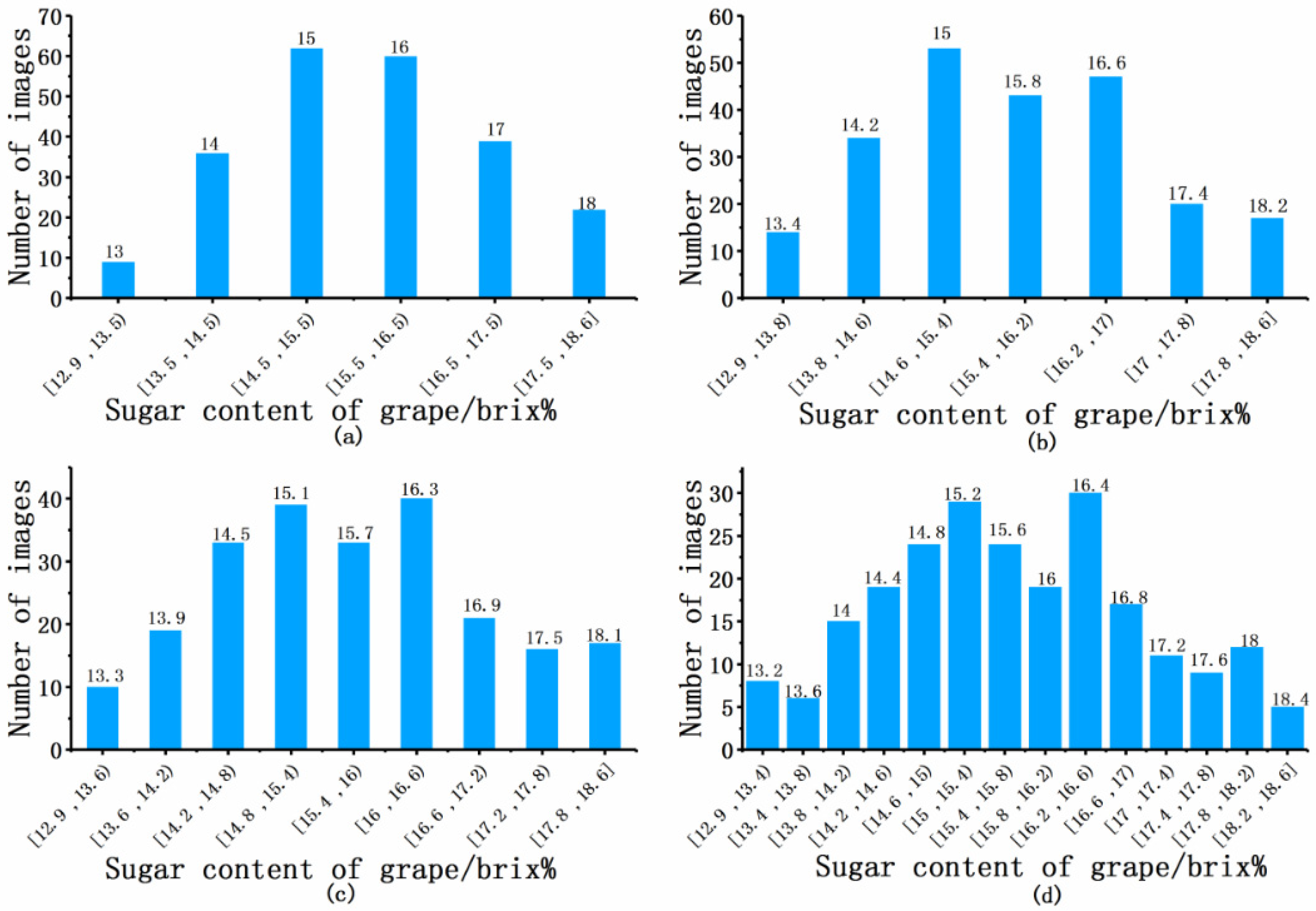
The grape dataset has an imbalanced distribution in terms of sugar content. The distribution of the collected grapes’ sugar content (Brix%) was 12.9~18.6. This study investigated the quality classification of the Red Globe grape. There are three times more datasets of grapes in the range of the 15~16% measure than grapes with the <14% or >18% measure. Standard data processing usually involves the characteristic that the number of samples in each category of the datasets is approximately uniformly distributed; this is called the category balance [11]. To address the non-uniform distribution issue, we divided the grape datasets to ensure the data were more uniformly distributed. We divided the data into 0.4%, 0.6%, 0.8%, and 1% intervals (Figure 3). Since the data in the certain interval are close to the label we defined, we can obtain the final regression result by operating on the label vector. The division method is simple and effective for the proposed FNRR network. We compared the performance of our method on the different interval divisions of the data to determine which resulted in the best performance. Image rotation was used for data augmentation [10] to make each set of data the same amount; left and right rotation was performed on the existing grape segmentation image, with a rotation angle between −20° and 20°.

Figure 3.
Imbalanced grape datasets. Datasets divided into intervals of (a) 1%, (b) 0.8%, (c) 0.6%, and (d) 0.4%. The value at the top of each bar is the average label for that category.
2.3. FNRR Network
In this experiment, we propose an innovative deep learning framework FNRR, shown in Figure 4, for the non-destructive prediction of the sugar content of grapes. The framework is mainly composed of two modules: (1) The feature extraction module, which obtains the feature vector to obtain the result of the normalized vector through convolutional neural networks or transformer models, and (2) the normalized function, which produces a categorical distribution from the previous layer’s output. The entries of the labeled vector are the average labels of each category. The result was achieved through the expectation of the normalized vector and labeled vector. The process of training is described in Algorithm 1 (The proposed algorithm for training the feature normalization reweighting regression models. Epoch is the number of iterations during training).
| Algorithm 1. Feature normalization reweighting regression model training |
| 1 for X=1; X<=Epoch; X++ |
| 2 Read a segmented grape image |
| 3 Put the image in deep learning model to obtain the Feature maps of the image |
| 4 Put the Feature maps in FC layer to obtain the matrix |
| 5 Normalize the matrix to obtain the Normalized Vector |
| 6 Compute the Output Vector with Normalized Vector and Label Vector |
| 7 Average the elements of Output Vector to obtain the final Brix Value of the image |
| 8 end for |
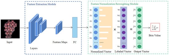
Figure 4.
Overview of the feature normalization reweighting regression (FNRR) model architecture.
Due to the non-uniform distribution of the data, the direct use of a multiple linear regression model will generate data a priori; the model will predict the data in the sparsely dense interval as if it were in the denser interval. The characteristics of the predicted data have a greater similarity to the data in the adjacent interval, and we can enrich the characteristics of the sparse interval data to a certain extent using grouping. We divided the grape image dataset into 14, 9, 7, and 6 categories with sugar content intervals of 0.4%, 0.6%, 0.8%, and 1%, respectively, and labeled each category with an appropriate sugar content value. We used typical deep learning-based models to obtain the features. A feature map is obtained by the convolution layer or attention mechanism. The convolution layer is composed of the kernel size, stride, padding, input channels, and output channels. For details, see Section 2.3.1. The image is operated with layers of encoder blocks based on the self-attention mechanism to obtain the feature maps. The self-attention mechanism is described in Section 2.3.3. The last layer of the model is a fully connected layer whose size is the number of the categories. The output result of the fully connected layer is passed through a normalized function, and a probability value is given to each category label; this is calculated as the expected value with the vector of the category label.
2.3.1. Convolutional Neural Network
A convolutional neural network is a typical feedforward neural network [12] and is particularly prominent in image recognition research. The basic architecture of a convolutional neural network usually consists of three parts: The convolutional layer, the pooling layer, and the fully connected layer. The purpose of the convolutional layer is to learn the input sample characteristics [13,14], while the pooling layer, which is also called a downsampling operation, aims to control the spatial distortion of the data and reduce the resolution of the feature map [15]; the pooling layer is usually located between two convolutional layers. After the convolutional neural network has gone through several convolution and pooling layers, one or more fully connected layers will be set.
2.3.2. Transfer Learning
Transfer learning uses the correlation between multiple domains to transfer the knowledge learned in the source domain to the target domain to assist in the training of the target model [16]. By combining source domain knowledge and target domain data, the model’s demand for the size of the target domain is reduced. It also allows the model to utilize the knowledge learned from other related tasks to assist the target task. Deep neural networks can automatically learn features from the original data; the lower layers of neural networks can learn detailed information, such as textures, and the higher layers can learn rich semantic information. Low-level features can be shared between many tasks; hence, transfer learning models can be reused directly. During the experiment, the model was pre-trained on the ImageNet dataset and was used as a feature extraction network to extract features from the input grape images [17].
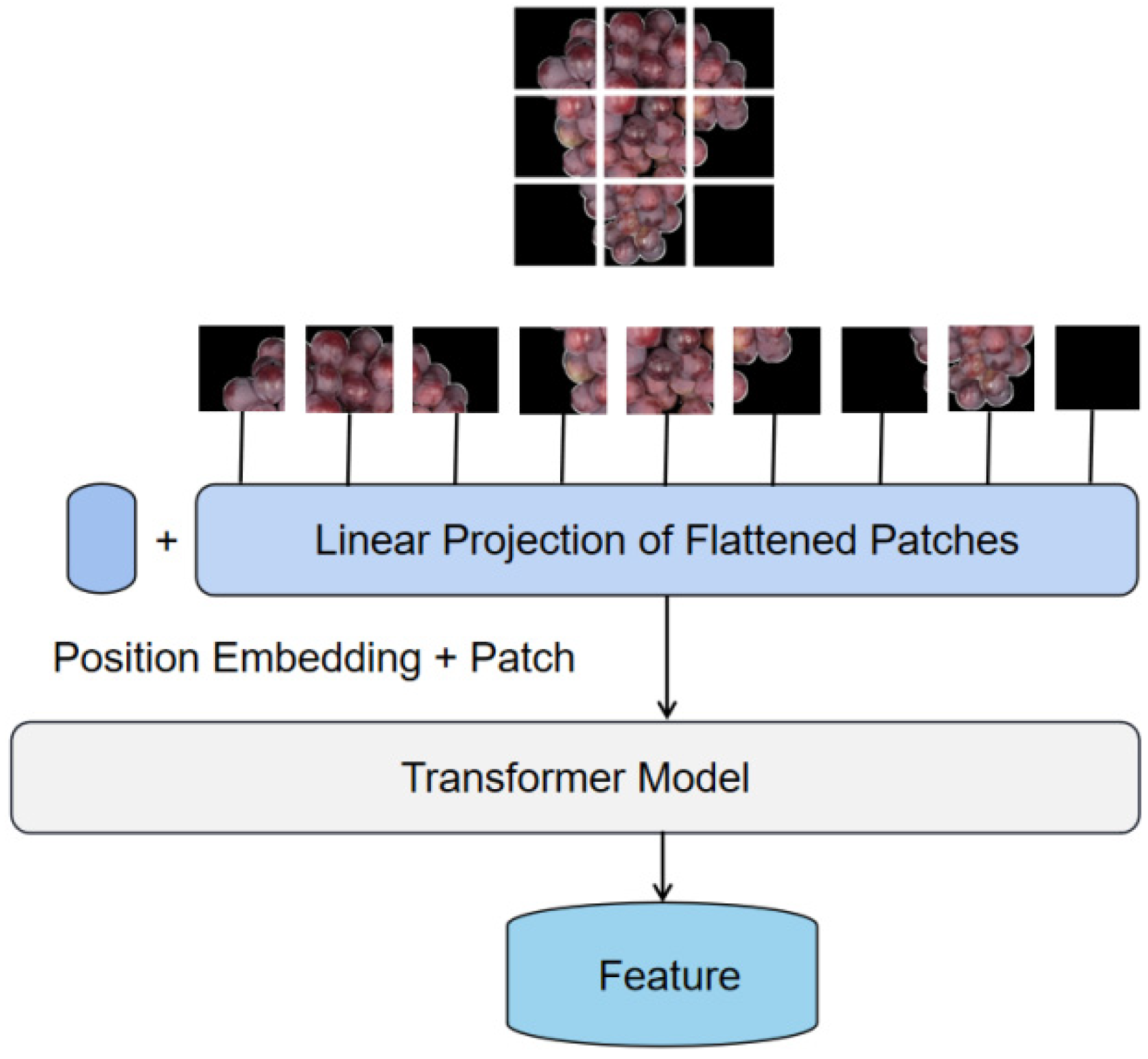
2.3.3. Transformer Model
A transformer model is a deep neural network, usually based on a self-attention mechanism, which was initially applied in the field of natural language processing. Inspired by its powerful representation capabilities, it was extended to computer vision tasks [18]. For visual tasks, convolutional neural networks have the advantage of inductive bias, translational equivalence, and locality; however, the model requires more convolutional layers to expand the receptive field. While the self-attention mechanism requires long-range information, it performs well for different visual tasks [19]. In Figure 5, the input grape image is divided into fixed-size patches, and patch embedding is performed using a linear transformation, with patch embedding indicating the image information and position embedding indicating the label information of the image from a sequence of token embeddings, taken as the transformer model’s input data [19]. The self-attention mechanism aggregates information by assigning different weights to the input information according to the current query. For a given query vector, k key vectors are matched using inner product calculation. The obtained inner product is then normalized using the softmax function to obtain k weights; the output of the query’s attention is the weighted average of the value vectors that correspond to the k key vectors [20]. The equation for this matrix calculation is given by
where:
- , , and : The three self-attention mechanism vectors.
- : The dimension of [20].
The transformer uses multi-head self-attention to define attention heads, i.e., self-attention is applied to the input sequence, which can be split into h sequences, and the outputs of the h different heads are then concatenated together. The final output is obtained using linear transformation [18]. The formula is defined as follows:
where:
- : The attention head obtained from Equation (1) [20].
- : Parameter matrices of the model.
In this experiment, we use the pre-trained transformer models to extract image features. Since the normalized feature is obtained from the classification model, we propose a multi-label loss function that compares the mean square error and cross-entropy with the loss of the mean square error, as described in Equations (4) and (5):
where:
- : Reference value.
- : Model estimate.
- : Probability of the category reference value.
- : Probability distribution of the category model estimate.
- : Number of images in one batch.
- : Size of the categories.
In this work, we find that the widely used MSE loss () function can be ineffective in imbalanced regression, so we propose a new balanced loss function from an imbalanced perspective to adapt to the label distribution of the imbalanced training set. The balanced loss function () has two parts: The first part is the standard MSE loss and the second part is a new balanced item. According to the data we constructed, each group of data achieved a balanced effect in quantity after amplification. Based on our proposed FNRR framework, we introduced the balance loss term cross-entropy and hyperparameter , which is obtained from multiple experiments.

Figure 5.
Grape feature extraction based on transformer model.
Figure 5.
Grape feature extraction based on transformer model.
2.4. Experimental Setting and Evaluation
In this study, we tested the performance of the FNRR framework on four grape datasets using three methods: Deep convolutional neural network retraining, transfer learning, and a transformer model. The experiment was conducted on ubuntu 16.04, equipped with NVIDIA GeForce GTX 1080TI. The R and RMSE are mainly used to evaluate the performance of each model based on the FNRR framework, and MaximumError is used for reference. A higher R indicated that the model was more stable, and a lower RMSE indicated a greater model accuracy. MaximumError is an absolute value of the difference between the label truth and the predicted value, which is a reference value. These values are defined as follows:
where:
- : Reference value.
- : Model estimate.
- : Covariance between and .: Respective standard deviations of y.
- : Respective standard deviations of .
- : The function to pick up the max number from the data.
3. Results and Discussion
3.1. Analysis of Convolutional Neural Network Retraining Results
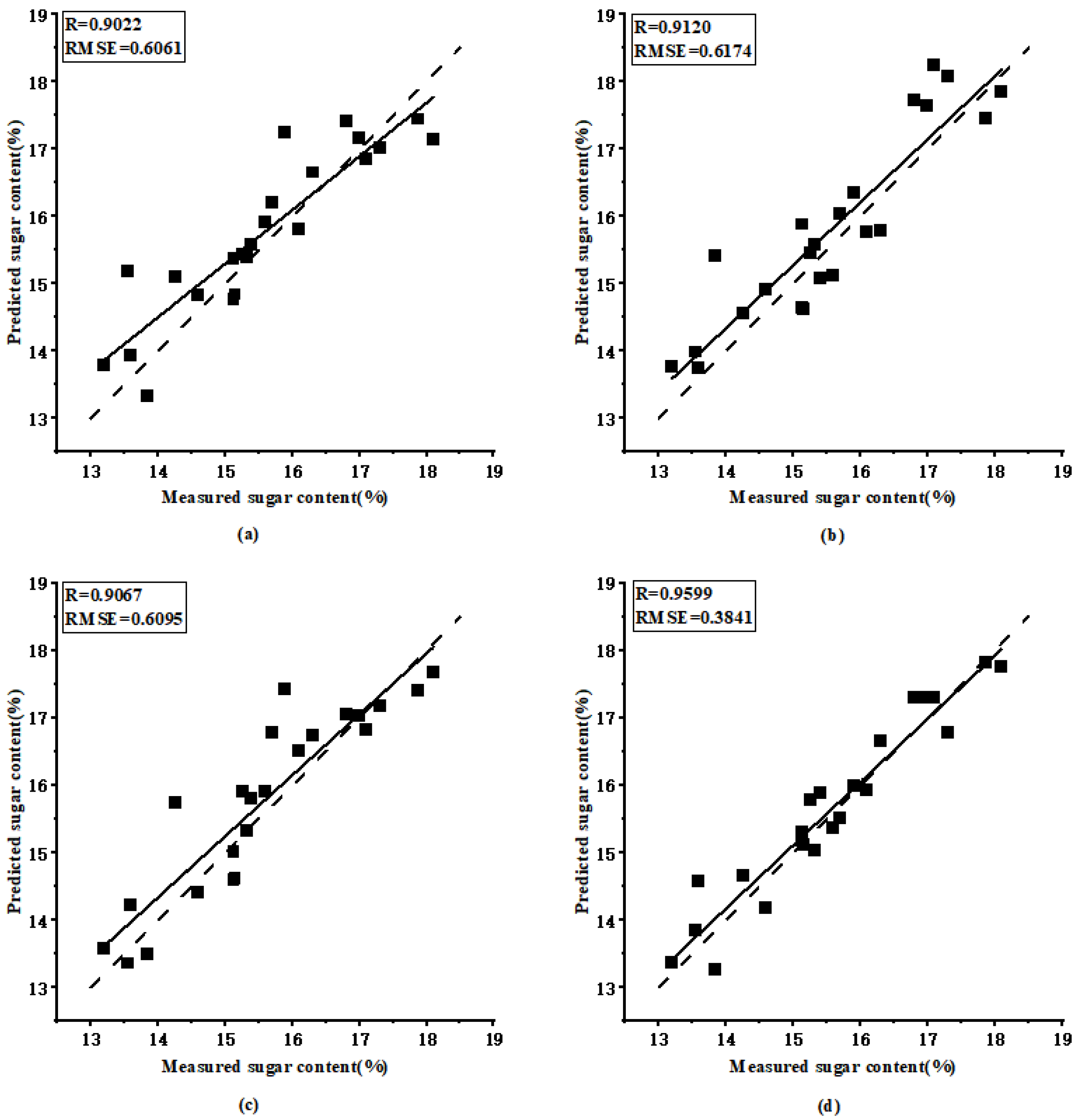
AlexNet [21] is a classic algorithm of convolutional neural networks. The small datasets were retrained from the outer to the end. Results showed that as the interval of the Brix measure was reduced, the became smaller. AlexNet yielded the best performance for an interval of 0.4 %, with = 0.9022 and = 0.6061%. In Table 1, the unstable results are not suitable for practical application due to the limitation of feature expression ability. However, transfer learning can provide more feature expression capabilities.

Table 1.
Comparison results of the models based on the loss1 function.
3.2. Analysis of Transfer Learning Results
The transfer learning method used in this study was an end-to-end model; this allowed the model to learn how to extract key features, and it was proven to be effective for small samples. The transfer learning networks ResNet50 [22] and InceptionV3 [23] were used in this experiment. Under the transfer learning method, the and ’s fluctuation ranges were relatively small on all four datasets (Table 1). For ResNet50, the difference between the maximum and minimum and was 0.0381 and 0.0891%, respectively. For InceptionV3, the difference between the maximum and minimum difference and was 0.0313 and 0.1499%, respectively. InceptionV3 obtained the best performance with intervals of 0.4%, with = 0.9120 and = 0.6174%. ResNet50 model obtained the best performance with intervals of 0.4%, with = 0.9067 and = 0.6095%.
3.3. Analysis of Transformer Model Result
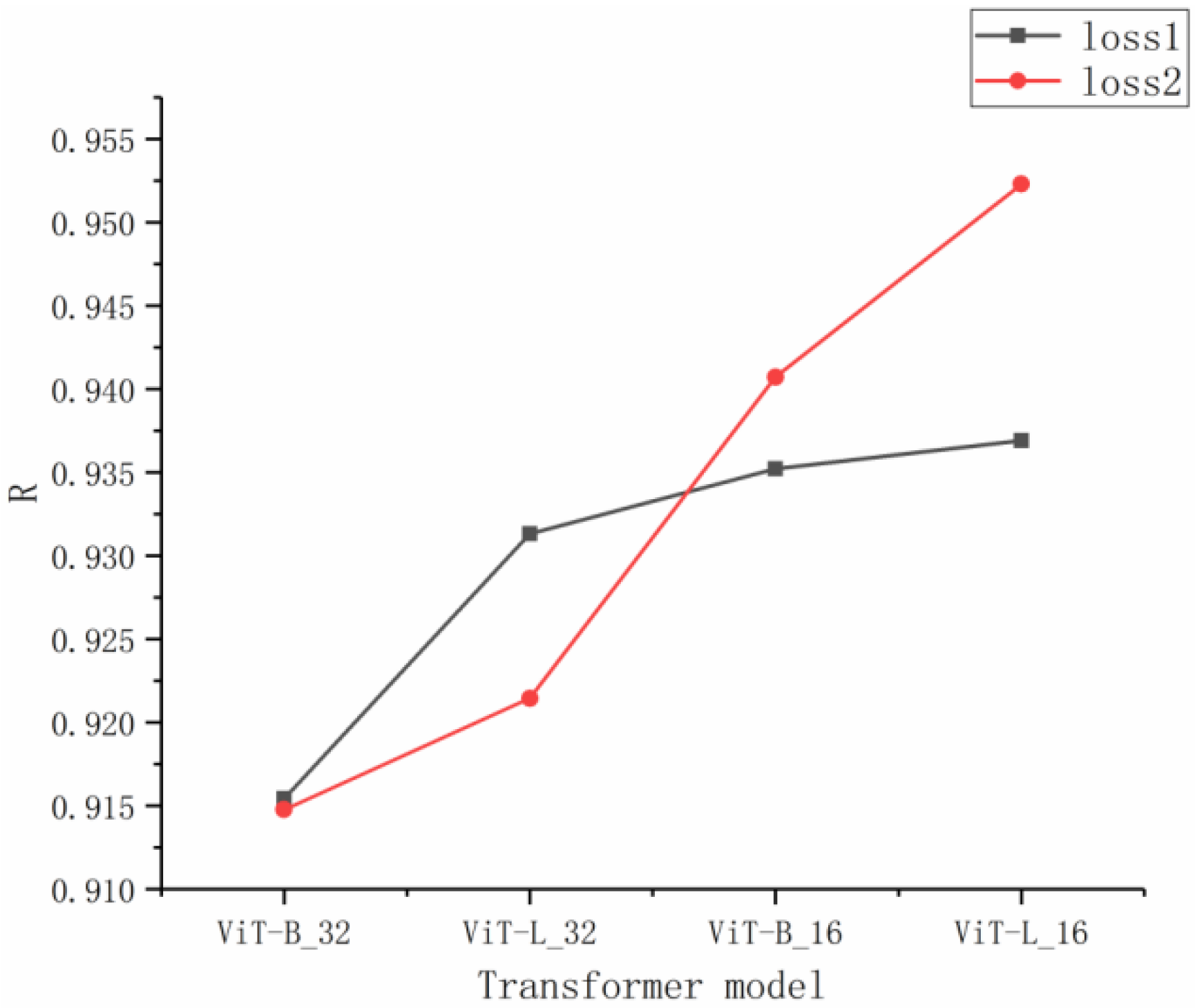
In this experiment, four transformer models were used for training: ViT-B_32, ViT-B_16, ViT-L_32, and ViT-L_16. The accuracy of the test set is shown in Table 2. Figure 6 shows the of the four transformer models, based on the average of the results of all four data division methods. Smaller patch sizes yield a better score with more layers. The model performed better overall with a patch size of 16. These results show that for grape samples of small size, the smaller the patch size, the better the model at feature extraction.
Table 2.
Comparison results of visual transformer models.

Figure 6.
of different transformer models based on the average of all four data division methods.
Table 2 suggests that three transformer models achieved the best results on the datasets with an interval of 0.6%, while the remaining models achieved the best results on datasets with an interval of 0.8%. Comparing the optimal model with the other models, there was a difference of 0.009 and 0.0019% in the and values for the datasets with an interval of 0.6%. This suggests that it was easier to obtain optimal results for the datasets with an interval of 0.6%.
Table 2 shows that, for the two models with a patch size of 16, the proposed loss2 has higher accuracy on the test set than the traditional loss1. The dataset with the 0.8% interval achieved the best results. In comparison with loss1, loss2 increased by 0.0444 and reduced by 0.182%. ViT-L_16 obtained the best performance with the datasets with a 0.8% interval, with = 0.9599 and = 0.3841%. The effect of the transformer model is significantly better than that of the classic convolutional neural network; the increased by 0.0577, and the was reduced by 0.2220%, compared to the AlexNet model that achieved the best result for the typical convolutional neural network model (Table 3). The visual analysis corresponding to Table 3 is shown in Figure 7. In addition, visual transformer models and typical convolutional neural network models each have consistency on a specific partition. Typical convolutional neural network models achieved the best performance on the interval of 0.4%. while the visual transformer models obtained optimal results more easily for the datasets with an interval of 0.6%.
Table 3.
Comparison of the best results for the typical convolutional neural network and visual transformer models.
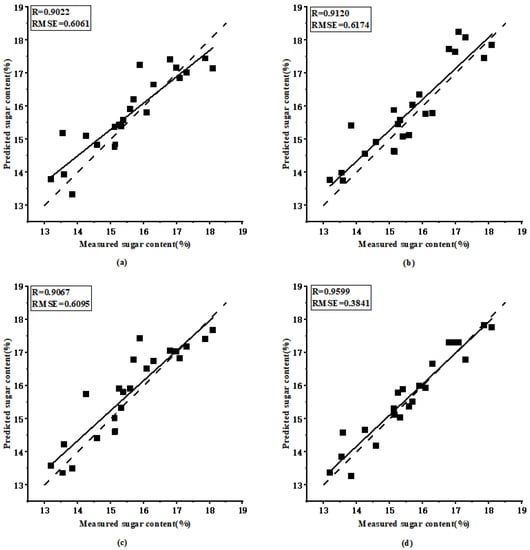
Figure 7.
Performance results using FNRR-net: (a) prediction results based on AlexNet model with the interval of 0.4% and MSE loss function, (b) prediction results based on InceptionV3 model with the interval of 0.4% and MSE loss function, (c) prediction results based on ResNet50 model with the interval of 0.4% and MSE loss function, (d) prediction results based on ViT-L_16 model with the interval of 0.8% and balanced loss function. The solid line is the fitting line between the predicted and measured values, and the dotted line is 1:1 line.
4. Conclusions
This study used deep learning technology to predict the sugar content of Red Globe grapes. The deep convolutional neural network retraining using AlexNet, the transfer learning method using InceptionV3 and ResNet50, and the transformer model can ensure the integrity of the grapes by accurately and effectively predicting the sugar content value. Furthermore, we designed a grape image acquisition system. However, the collected dataset of grapes presented an imbalanced distribution. We proposed the FNRR framework to address this issue and demonstrate that it performed well on small samples of grapes with an imbalanced distribution. In addition, under our proposed multi-label loss function, and among all prediction models, the FNRR framework in conjunction with the ViT-L_16 transformer and the dataset categorized with intervals of 0.8% yielded the optimal performance, with = 0.9599 and = 0.3841%. Using transformer models to predict the sugar content of grapes is a potential method for the non-destructive quality testing and grading of grapes. In future studies, we aim to enrich our dataset to make it applicable to other fruits and apply the FNRR framework to industrial production.
Author Contributions
Conceptualization, funding acquisition, J.L. (Jun Luo); methodology, T.H.; software, J.L. (Jiuliang Li); validation, formal analysis, Y.J.; investigation, resources, data curation, writing—original draft preparation, writing—review and editing, visualization, supervision, project administration, M.J. All authors have read and agreed to the published version of the manuscript.
Funding
The Fundamental Research Funds for the Central Universities (grant nos. 2662022XXYJ006, 2662017PY059 and 2662015PY066), the National Natural Science Foundation of China (grant nos. 61176052 and 61432007), and the Cooperation funding of Huazhong Agricultural University-Shenzhen Institute of Agricultural Genomics, Chinese Academy of Agricultural Sciences (HZAU-AGIS Cooperation Fund SZYJY2021011).
Institutional Review Board Statement
Not applicable.
Informed Consent Statement
Not applicable.
Data Availability Statement
Data are available on request from the authors.
Conflicts of Interest
The authors declare no conflict of interest.
References
- Failla, O.; Mariani, L.; Brancadoro, L.; Minelli, R.; Scienza, A.; Murada, G.; Mancini, S. Spatial distribution of solar radiation and its effects on vine phenology and grape ripening in an alpine environment. Am. J. Enol. Vitic. 2004, 55, 128–138. Available online: https://www.ajevonline.org/content/55/2/128 (accessed on 15 February 2022).
- Meng, X. The Effect of Light Intensity on the Fruit Coloration of Red Globe Grape. Master’s Thesis, ShiHeZi University, ShiHeZi, China, 2014. [Google Scholar] [CrossRef]
- Ren, G.; Tao, R.; Wang, C.; Sun, X.; Fang, J. Study on the relationship between grape berry coloration and UFGT and MYBA gene expression. J. Nanjing Agric. Univ. 2013, 36, 7. Available online: https://kns.cnki.net/kcms/detail/detail.aspx?dbcode=CJFD&dbname=CJFD2013&filename=NJNY201304007&uniplatform=NZKPT&v=tE8aZGJ3GHOHn8LxUnPIDvxqwNSNxBowlOqTcGASZvAFC2nwH65Rj-WjOT-Ex1lF (accessed on 15 February 2022).
- Hernández-Hernández, J.L.; García-Mateos, G.; González-Esquiva, J.M.; Escarabajal-Henarejos, D.; Ruiz-Canales, A.; Molina-Martínez, J.M. Optimal color space selection method for plant/soil segmentation in agriculture. Comput. Electron. Agric. 2016, 122, 124–132. [Google Scholar] [CrossRef]
- García-Mateos, G.; Hernández-Hernández, J.; Escarabajal-Henarejos, D.; Jaén-Terrones, S.; Molina-Martínez, J. Study and comparison of color models for automatic image analysis in irrigation management applications. Agric. Water Manag. 2016, 151, 158–166. [Google Scholar] [CrossRef]
- Huang, Y.; Wang, J.; Li, N.; Yang, J.; Ren, Z. Predicting soluble solids content in “Fuji” apples of different ripening stages based on multiple information fusion. Pattern Recognit. Lett. 2021, 151, 76–84. [Google Scholar] [CrossRef]
- Sajad, S.; Ignacio, A. A visible-range computer-vision system for automated, non-intrusive assessment of the pH value in Thomson oranges. Comput. Ind. 2018, 99, 69–82. [Google Scholar] [CrossRef]
- Kondo, N.; Ahmad, U.; Monta, M.; Murase, H. Machine vision based quality evaluation of Iyokan orange fruit using neural networks. Comput. Electron. Agric. 2000, 29, 135–147. [Google Scholar] [CrossRef]
- Tang, Y. Research on the Non-Destructive Testing Technology of Red Grape Quality. Huazhong Agricultural University. 2016. Available online: https://kns.cnki.net/kcms/detail/detail.aspx?dbcode=CMFD&dbname=CMFD201701&filename=1016155352.nh&uniplatform=NZKPT&v=XQela6bRTxRWG2NKHwRnHPcVxpEJRfMwPKWe47FZCBhrdGzlLRsbionCK3lVKI6a (accessed on 15 February 2022).
- Ronneberger, O.; Fischer, P.; Brox, T. U-Net: Convolutional Networks for Biomedical Image Segmentation. Med. Image Comput. Comput-Assist. Interv. 2015, 9351, 234–241. [Google Scholar] [CrossRef] [Green Version]
- Oksuz, K.; Cam, B.C.; Kalkan, S.; Akbas, E. Imbalance Problems in Object Detection: A Review. IEEE Trans. Pattern Anal. Mach. Intell. 2020, 43, 3388–3415. [Google Scholar] [CrossRef] [PubMed] [Green Version]
- Shorten, C.; Khoshgoftaar, T. A survey on Image Data Augmentation for Deep Learning. J. Big Data 2019, 6, 60. [Google Scholar] [CrossRef]
- Lecun, Y.; Bottou, L. Gradient-based learning applied to document recognition. Proc. IEEE 1998, 86, 2278–2324. [Google Scholar] [CrossRef] [Green Version]
- Simonyan, K.; Zisserman, A. Very Deep Convolutional Networks for Large-Scale Image Recognition. In Proceedings of the 3rd International Conference on Learning Representations, ICLR 2015, San Diego, CA, USA, 7–9 May 2015; Available online: https://arxiv.org/abs/1409.1556 (accessed on 15 February 2022).
- Lin, M.; Chen, Q.; Yan, S. Network in network. In Proceedings of the International Conference for Learning Representations (ICLR), Banff, AB, Canada, 14–16 April 2014; Available online: https://arxiv.org/abs/1312.4400 (accessed on 15 February 2022).
- Weiss, K.; Khoshgoftaar, T.; Wang, D. A survey of transfer learning. J. Big Data 2016, 3, 9. [Google Scholar] [CrossRef] [Green Version]
- Ioffe, S.; Szegedy, C. Batch Normalization: Accelerating Deep Network Training by Reducing Internal Covariate Shift. In Proceedings of the 32nd International Conference on International Conference on Machine Learning, Lille, France, 6–11 July 2015; Volume 37, pp. 448–456. [Google Scholar] [CrossRef]
- Khan, S.; Naseer, M.; Hayat, M.; Zamir, S.W.; Khan, F.S.; Shah, M. Transformers in Vision: A Survey. ACM Comput. Surv. 2021. [Google Scholar] [CrossRef]
- Dosovitskiy, A.; Beyer, L.; Kolesnikov, A.; Weissenborn, D.; Zhai, X.; Unterthiner, T.; Dehghani, M.; Minderer, M.; Heigold, G.; Gelly, S.; et al. An Image is Worth 16 × 16 Words: Transformers for Image Recognition at Scale. In Proceedings of the 9th International Conference on Learning Representations, Virtual Event, Austria, 3–7 May 2021; Available online: https://openreview.net/forum?id=YicbFdNTTy (accessed on 15 February 2022).
- Vaswani, A.; Shazeer, N.; Parmar, N.; Uszkoreit, J.; Jones, L.; Gomez, A.N.; Kaiser, L.; Polosukhin, I. Attention is All you Need. ArXiv. In Proceedings of the 31st Conference on Neural Information Processing Systems (NIPS 2017), Long Beach, CA, USA, 4–9 December 2017; Available online: https://arxiv.org/abs/1706.03762 (accessed on 15 February 2022).
- Krizhevsky, A.; Ilya, S.; Hinton, G. Imagenet classification with deep convolutional neural networks. In Advances in Neural Information Processing Systems; Curran Associates Inc.: Red Hook, NY, USA, 2012; Volume 1, pp. 1097–1105. [Google Scholar] [CrossRef]
- He, K.; Zhang, X.; Ren, S.; Sun, J. Deep Residual Learning for Image Recognition. In Proceedings of the 2016 IEEE Conference on Computer Vision and Pattern Recognition (CVPR), Las Vegas, NV, USA, 27–30 June 2016; pp. 770–778. [Google Scholar] [CrossRef] [Green Version]
- Szegedy, C.; Vanhoucke, V.; Ioffe, S.; Shlens, J.; Wojna, Z. Rethinking the Inception Architecture for Computer Vision. In Proceedings of the 2016 IEEE Conference on Computer Vision and Pattern Recognition (CVPR), Las Vegas, NV, USA, 27–30 June 2016; pp. 2818–2826. [Google Scholar] [CrossRef] [Green Version]
Publisher’s Note: MDPI stays neutral with regard to jurisdictional claims in published maps and institutional affiliations. |
© 2022 by the authors. Licensee MDPI, Basel, Switzerland. This article is an open access article distributed under the terms and conditions of the Creative Commons Attribution (CC BY) license (https://creativecommons.org/licenses/by/4.0/).