Abstract
Helminthiasis disease is one of the most serious health problems in the world and frequently occurs in children, especially in unhygienic conditions. The manual diagnosis method is time consuming and challenging, especially when there are a large number of samples. An automated system is acknowledged as a quick and easy technique to assess helminth sample images by offering direct visibility on the computer monitor without the requirement for examination under a microscope. Thus, this paper aims to compare the human intestinal parasite ova segmentation performance between machine learning segmentation and deep learning segmentation. Four types of helminth ova are tested, which are Ascaris Lumbricoides Ova (ALO), Enterobious Vermicularis Ova (EVO), Hookworm Ova (HWO), and Trichuris Trichiura Ova (TTO). In this paper, fuzzy c-Mean (FCM) segmentation technique is used in machine learning segmentation, while convolutional neural network (CNN) segmentation technique is used for deep learning. The performance of segmentation algorithms based on FCM and CNN segmentation techniques is investigated and compared to select the best segmentation procedure for helminth ova detection. The results reveal that the accuracy obtained for each helminth species is in the range of 97% to 100% for both techniques. However, IoU analysis showed that CNN based on ResNet technique performed better than FCM for ALO, EVO, and TTO with values of 75.80%, 55.48%, and 77.06%, respectively. Therefore, segmentation through deep learning is more suitable for segmenting the human intestinal parasite ova.
1. Introduction
Helminthiasis remains one of the serious public health concerns that affects millions of people in the world including Malaysia. The global report indicates that more than 1.5 billion people are diagnosed with helminthiasis through soil-transmitted helminth infection, representing 24% of the worldwide population [1]. The Ascaris Lumbricoides species affects the most people with an estimated 807–1121 million, followed by the Trichuris Trichiura species with approximately 604–795 million and Hookworm species with around 576–740 million [2]. Children between the ages of 5 and 15 are particularly vulnerable to infection, which can have a negative impact on their physical, mental, and emotional well-being [3]. In 2020, more than 436 million children in the world were treated for helminthiasis disease [1].
Helminth infection is transmitted to human beings through the soil, water, food, and molluscan vectors. After the contamination of soil by human or animal feces, the helminth ovum or larvae begins to develop and survive in soil with a favorable environment. Upon skin contact with tainted soil or ingestion of polluted soil, water, or food, people will become infected. Patients with light helminth infections usually do not suffer from symptoms whereas patients with heavier infections will suffer from symptoms including diarrhea, abdominal pain, chronic intestinal blood loss, anemia, loss of appetite, weakness, and malnutrition. Helminth worms absorb nutrients from the host tissue, which includes blood, this causes massive iron and protein loss in the human body [4]. Helminth not only infects the intestine but also other organs including the liver, brain, lungs, and blood [5]. Helminth infection can be life threatening if not diagnosed and treated immediately, especially in children and pregnant women.
Usually, manual observation under a microscope is one of the methods used by parasitologists to detect the different types of helminth ova. Based on the size and structure of the helminth ovum, identification for the types of helminth can be conducted. However, the microscopic samples are generally embedded with unnecessary components that share common traits including color and shape with the helminth ova. Hence the ova are easily mistakenly identified. Thus, it will reduce the accuracy of diagnosis. Moreover, this manual observation method is inefficient when there are many samples. This is due to humans having limitations on accurately observing the samples in a specific period. In addition, this examination method is very time consuming and costly due to the complicated procedures. These approaches are not suitable for field surveys or the rapid identification of those most in need of treatment [6].
Many image processing and classification techniques have been approached to recognize the helminth species either by using machine learning or deep learning to overcome these manual observation limitations. These image processing and classification techniques using machine learning and deep learning will be set up in the computerized microscopic lab in order to help the deliverability to medically underserved communities.
Machine learning is the scientific study of algorithms and statistical models that computer systems use to perform a specific task without being explicitly programmed. It is used to teach machines how to handle the data more efficiently [7]. A machine learning system was proposed by Jimenez [8], which identifies and quantifies seven species of helminth in wastewater at different development stages. In the preprocessing stage, grey-scale conversion, anisotropic diffusion filter, and Gaussian derivative function with image binarization were applied to enhance the outer shell of the ova and segment the image. A naïve Bayesian classifier was used and obtained a specificity of 99% and a sensitivity of 84%.
In deep learning, there are several neural networks such as convolutional neural network (CNN) and recurrent neural network (RNN). CNN has achieved great success in overcoming machine learning problems, especially when dealing with image datasets. Osaku et al. [9] presented a hybrid method to diagnose 15 types of human intestinal parasites in Brazil. This hybrid method is a combination of decision systems, DS1 and DS2, which are p-SVM and VGG-16, respectively. By combining two different decision systems, which is a faster but less accurate decision system DS1, and a slower but more accurate decision system DS2, the parasites are successfully detected and classified. The hybrid system can achieve Cohen’s Kappa of 94.9%, 87.8%, and 92.5% on helminth ova. A convolutional neural network (CNN) was used by Kitvimonrat et al. [10] to detect the parasite ova. Three types of architecture are used, which are Faster R-CNN, RetinaNet, and CenterNet. The classification accuracy for RetinaNet is 83%.
Based on previous studies [8,9,10], segmentation plays a major role in achieving good performance for helminth ova detection. Thus, this paper presents the comparison in segmentation performance achieved between machine learning and deep learning in segmenting the human intestinal parasite ova.
2. Materials and Methods
In this paper, the procedure is divided into two parts, which are machine learning and deep learning. Figure 1 shows the illustration for the flow chart of the techniques proposed in machine learning and deep learning procedure.
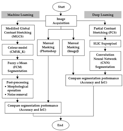
Figure 1.
Flow chart for the techniques proposed for machine learning and deep learning segmentations.
2.1. Image Acquisition
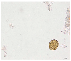
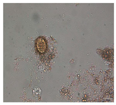
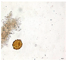
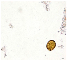
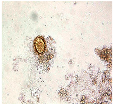
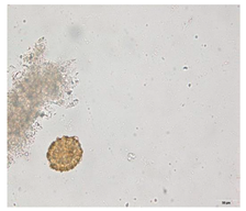
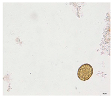
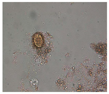
A computerized microscope was utilized to capture helminth ovum images with different species, which are Ascaris Lumbricoides Ova (ALO), Enterobious Vermicularis Ova (EVO), Hookworm Ova (HWO), and Trichuris Trichiura Ova (TTO) from the feces sample slide. The Department of Microbiology and Parasitology from Hospital Universiti Sains Malaysia (HUSM) prepared these feces samples, which were freshly obtained from the helminthiasis patients. The feces slides were observed under 40× magnification and saved to JPG extension with a dimension of 1249 × 980. The total images collected were 664 different images with no overlapping data, which have 166 images for each species, that is, 100 images for normal, 33 images for under-exposed, and 33 images for over-exposed illuminations. The illumination of the images is set up through the microscope lighting with the guidance of the parasitologist.
2.2. Machine Learning Segmentation Approach
2.2.1. Modified Global Contrast Stretching (MGCS)
The MGCS enhancement technique was used to standardize the illumination and also to enhance the helminth ova image. The MGCS technique uses a value from the pixel percentage based on the overall amount of pixels in the helminth image to create new minimum and maximum values for each of the R, G, and B components [11]. The percentage of the minimum value () is obtained from the lowest value among the R, G, and B color components out of the total numbers of pixels, likewise for the maximum value . The lowest and highest values obtained must satisfy the conditions in Equations (1) and (2).
where and are the total amounts of pixels that fall between a particular minimum and maximum percentage, while and are the preferred values for minimum and maximum percentage.
2.2.2. Color Model
Next, the color model is used in the machine learning segmentation procedure to make the targeted region distinct and reduce the unwanted artifacts regions on the helminth image. Thus, the K component from CMYK (CMYK_K) color model is applied to the enhanced helminth ova images. Equations (3) and (4) show the calculations in obtaining the K component from the RGB image.
2.2.3. Fuzzy c-Mean (FCM) Segmentation
The FCM clustering algorithm is an iterative distributing technique that yields optimal c-partitions. This technique calculates the cluster centers and produces the class membership matrix. The generalized least-squared error function is minimized via the optimal fuzzy c-partition. The initial random membership matrix is generated through the algorithm of FCM. This random membership matrix is used as the weight for each sample to fit in each cluster. Then, the centroid for each cluster is calculated using Equation (5). The membership matrix is updated through the generated new cluster centers. Then, the updated membership matrix is compared to the previous membership matrix. If the difference exceeds a certain threshold, then another iteration is generated. Otherwise, the algorithm is stopped [12].
where the is the minimized FCM, meanwhile, is the data set. is the number of clusters in , and m is the weighting exponent. Then, is the fuzzy c-partition for . While is an induced a-norm of .
2.2.4. Post-Processing
After image segmentation, these segmented helminth images undergo post-processing procedures that contain several morphological operations such as opening, closing, and filling holes. These methods are used to recover the information lost during the segmentation procedure. However, the tendency for the unwanted region to reappear is still there. Therefore, the object remover technique is used to remove the image pixels that are smaller than the size of the desired segmented image to avoid miss-identifying the helminth species. The size of helminth ova for the four species images, in between 6000 pixels to 38,000 pixels, is identified by trial-and-error analysis. Thus, any segmented regions that are less than 6000 pixels and more than 38,000 pixels are considered as unwanted regions and are removed during object removing operation.
2.2.5. Segmentation Performance
Both machine learning and deep learning used accuracy and Intersection over Union (IoU) metrics to analyze the quality of the segmented image produced. This analysis is done based on the pixel similarity by comparing the results of the segmented image against the ground truth. Therefore, the results obtained from the post-processing performance in machine learning are compared with the ground truth obtained from manual masking using Photoshop software.
The formula of accuracy requires the expected mask for pixel-level classification as true positive (TP), true negative (TN), false positive (FP), and false negative (FN). TP is denoted as detecting the correct helminth object, TN is denoted as detecting no object, FP is denoted as detecting the extra objects and FN is denoted as detecting the overlooked object [13]. The equation for the accuracy is shown in Equation (6).
The intersection of two sets divided by their union is defined by the IoU score, often known as the Jaccard index. If both the predicted mask and ground truth are similar, then the intersection is equal to the union, resulting in an IoU score of 100% achieved. In semantic segmentation research, an IoU result over 50% is usually regarded as a good prediction [14]. The equation for the accuracy is shown in Equation (7).
where GT represents the ground truth image while P represents the predicted image by the model.
2.3. Deep Learning Segmentation Approach
2.3.1. Partial Contrast Stretching (PCS)
The PCS technique was utilized to enhance the helminth ova images as it is a linear mapping function that is commonly used to increase the brightness and contrast level of the image [15]. This technique will enhance the image based on the original contrast and brightness level even with different illumination. The mapping formula can be given mathematically, as shown in Equation (8).
where is the color level of the output pixel, is the color level of the input pixel, is the maximum color level values in the input image, is the minimum color level in the input image and and are the desired maximum and minimum [16].
2.3.2. Simple Linear Iterative Clustering (SLIC) Superpixel
SLIC Superpixel is a k-mean adaptation technique for superpixel generation. The SLIC method calculated the distance from each cluster center to pixels within the 2S × 2S region, whereas the conventional k-mean clustering technique calculated the distance from each cluster center to all the pixels in the images. The SLIC algorithm helps to increase the segmentation performance in the CNN algorithm [17,18]. Therefore, it is used in this work to execute the segmentation of helminth ova and artifacts in images as a presegmentation method. The SLIC method used in this segmentation process depends on the pixel intensity values, which are the pixel values of RGB and the spatial distance of the pixel, which is the x and y coordinate information to the superpixel center [19]. The process formed by SLIC segmentation into each pixel in the image is shown in Equation (9).
where j represents the center pixel, i represents the value to be clustered, represents the distance of the corresponding pixel to the center, and r, g, b represent the brightness values of the pixel [20]. Equation (10) shows the distance of the coordinate of each pixel to the cluster center.
where and are the horizontal and vertical coordinate information of each center pixel, and and are the coordinate information of each pixel to be clustered. Equation (11) represents the simplified distance of the coordinate of each pixel to the cluster center.
where is the sum of the (x, y) plane distance normalized by the grid interval N and the lab distance. The parameter m is defined as the compactness of superpixels and it is allowed to weigh the relative importance between color similarity and spatial proximity [21]. The higher the value of m, the more compact the shape of the superpixel. In contrast, the lower the value of m, the shape of the superpixel will appear in less regular shape and size.
In this paper, the number of the superpixels, k, of the image was adjusted to 1000 while the compactness of the superpixel, m, was adjusted to 5. The chosen number of superpixels, k, is significant as it can determine the number of vectors. A small k value does not provide a sufficient signature, while a large k value will cause over-fitting and increase complexity [21].
2.3.3. CNN Semantic Segmentation
In this paper, semantic image segmentation will be carried out through CNN. Semantic segmentation will classify all the meaningful pixels into the same object classes. There are six basic steps in the basic CNN algorithm, including input layers, convolutional layers, rectified linear unit (ReLU), pooling layer, fully connected layer, and classification layer. In the input layer stage, each image needs to resize and be converted from grayscale to color image if necessary. At the convolutional layer, each image is convolved with k number of generalized kernels to create activation maps. The ReLU layer, also known as an activation layer, is used to transfer the activation maps to a nonlinear plane. Next, the pooling layer is used to reduce the number of parameters especially when the input image is too huge. A fully connected layer provides the correlations of the particular class to the high-level features. The number of outputs of the last fully connected layer must be the same as the number of classes. The classification layer is the final output layer in the CNN algorithm, also defined as a softmax layer that can perform multi-class classification [22].
The CNN used for deep learning focused on the U-Net model. U-Net was designed specifically for medical image analysis to segment the images accurately with a limited amount of training data [23]. The encoder part of the U-Net model is substituted by pretrained backbone models, which are VGG and ResNet. The backbone model acts as a feature extractor and it is used without the dense layers. In this paper, three backbones were proposed for evaluation, which are VGG-16, ResNet-18, and ResNet-34.
Then, the data split ratio was used for parameter tuning and was split into two groups, which are the training and validation datasets. The training dataset is the dataset on which the model is trained, these data are seen and learned by the model. The validation dataset is the dataset that is used to provide an unbiased evaluation of the model. In this paper, the data split ratio are adjusted to 0.1, which means 10% of the dataset is utilized as the validation dataset while 90% is considered as the training dataset. The 10% of the validation dataset acts as a holdout dataset to properly assess the performance.
2.3.4. Segmentation Performance
The results obtained from the CNN performance are compared with the ground truth obtained from manual masking using ImageJ software [21]. ImageJ software is a freeware tool and has been widely utilized by biologists for its utility and ease of use in handling many sorts of image data across numerous computing systems. Performance for the segmented image obtained from the deep learning procedure is measured through the comparison with the manual masking image using accuracy and IoU analysis.
3. Results and Discussion
A total of 664 images were collected from the ALO, EVO, HWO, and TTO species. Two types of segmentation techniques were applied, which are machine learning and deep learning. The results obtained by each technique are presented and analyzed in Section 3.1 and Section 3.2.
3.1. Machine Learning Segmentation
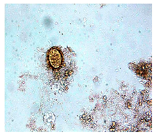
In machine learning segmentation, the sequence of the technique used is MGCS enhancement, CMYK_K color model, FCM segmentation, and post-processing. Table 1 displays the example of the ALO species captured in three different illuminations with the results obtained when the MGCS technique was implemented. The MGCS enhancement can standardize the illumination for the helminth images captured even though it comes in three different illuminations: normal illumination, under-exposed illumination, and over-exposed illumination. The enhanced image has shown better differentiation between the background and the helminth ovum.

Table 1.
ALO image before and after implementing the MGCS technique. Scale bar = 50 µm.
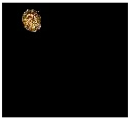
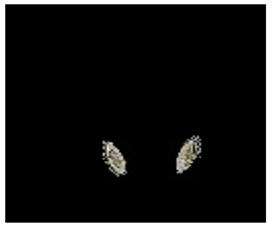
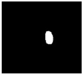
Next, the K component of the CMYK_K color model and FCM segmentation were implemented on the enhanced helminth ovum image. Both of these techniques can distinguish and separate the region of interest (ROI), which is the helminth ovum from the artifact and background. The post-processing procedure, based on morphological operations such as dilation, filling holes, and noise removal, is used to obtain a clean and clear segmentation image. Figure 2 shows the resultant image achieved after the CMYK_K color model and FCM were executed to the TTO image. Through the results obtained, a clean and clear segmented TTO image was produced. However, an artifact has also been segmented, which will affect the segmentation performance.

Figure 2.
The results of machine learning segmentation technique on TTO image: (a) MGCS on TTO image; (b) CMYK_K color model on enhanced TTO image; (c) FCM segmentation on TTO image; (d) Post-processing on TTO image. Scale bar = 50 µm.
3.2. Deep Learning Segmentation
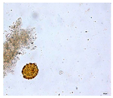
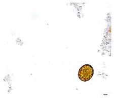
In deep learning segmentation, the sequence of the techniques used are PCS enhancement, SLIC superpixel, and CNN semantic segmentation. Table 2 shows the example of the ALO species captured in three different illuminations with the results obtained when the PCS technique was implemented. Through the enhancement results obtained, the contrast and brightness of the enhanced images were increased significantly. The enhanced image has shown better differentiation between the background and the helminth ovum. However, the background color was slightly changed. Even though this situation happens, it does not affect the next procedure as the helminth ovum can be seen clearly.
Table 2.
The ALO image before and after implementing PCS technique. Scale bar = 50 µm.
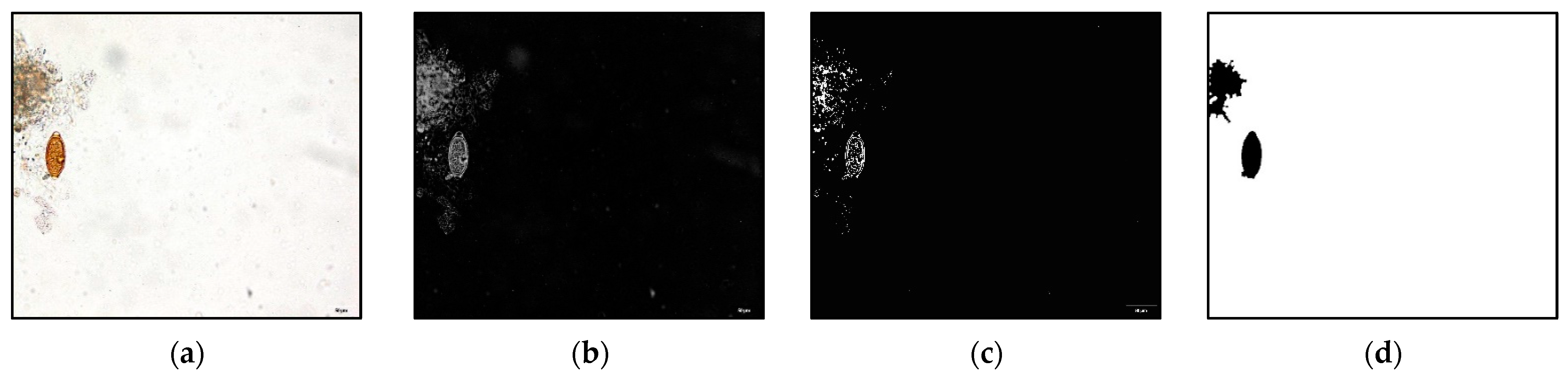
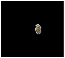
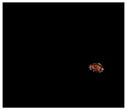
After that, the SLIC superpixel technique together with CNN segmentation was applied to the enhanced image. The resultant image obtained was used as the input for the CNN segmentation. Then, the CNN segmentation was applied through three different backbones, which are VGG-16, ResNet-18, and ResNet-34. A clean and clear image has been obtained. Figure 3 shows the resultant image achieved for the deep learning segmentation based on TTO image.
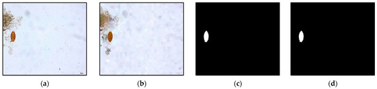
Figure 3.
The results of deep learning segmentation technique on TTO image: (a) PCS on TTO image; (b) SLIC superpixel technique on enhanced TTO image; (c) ResNet-18 on TTO image; (d) ResNet-34 on TTO image. Scale bar = 50 µm.
3.3. Segmentation Performances
An analysis based on the quantitative measure was performed between machine learning segmentation versus deep learning segmentation to identify the best segmentation performance for the helminth ova images. Table 3 tabulated the overall segmentation results obtained for the overall segmented helminth ova images based on accuracy and IoU analysis.
Table 3.
Quantitative measure for the segmentation performance of helminth ova images.
Based on Table 3, different species datasets have different results in segmentation performance, which are presented in the accuracy performance and IoU performance. Deep learning segmentation, based on ResNet-34, has achieved the highest results for accuracy and IoU for the ALO species with 99.30% and 75.80% each. For the EVO species, deep learning segmentation based on VGG-16 has achieved the highest accuracy results with a value of 98.89%, and ResNet-34 achieved the highest results for the IoU with a value of 55.48%. Meanwhile, machine learning segmentation based on FCM has achieved the highest results for both accuracy and IoU with values of 99.48% and 73.25% each for the HWO species. Then, for the TTO species, deep learning segmentation based on VGG-16 has achieved the highest results for accuracy and deep learning segmentation based on ResNet-18 has achieved the highest results for IoU.
Through the results obtained for accuracy, both segmentation techniques show good segmentation performances, which are around 97% to 100% in segmenting the helminth ova. Meanwhile, in IoU analysis, most of the segmentation techniques show results higher than 50%, which indicates that the helminth ova are well segmented, but there is significant contrast between the results obtained by machine learning segmentation and deep learning segmentation.
Table 4 shows an example of the segmentation performance achieved by deep learning segmentation for accuracy and IoU via ResNet-34 for helminth ova. Through the example shown, the IoU analysis is more sensitive than the accuracy analysis. Therefore, a good segmented image will achieve higher IoU analysis when compared to the ground truth image. Overall, deep learning segmentation has shown better segmentation results for both accuracy and IoU compared to machine learning segmentation. The results obtained are a good benchmark in developing an automatic detection system for helminth ova in the human intestine.
Table 4.
Segmentation performance of helminth ova images for ResNet-34.
4. Conclusions
The work presented in this paper compared the segmentation performance of machine learning and deep learning when applied to the four helminth ova species based on human intestinal parasite ova, which are ALO, EVO, HWO, and TTO. Through the segmentation performance achieved, the deep learning segmentation procedure is more suitable to segment the helminth ova compared to the machine learning segmentation. However, there are still some flaws that should be improved so that the segmentation performance can have a better value.
This work serves as an initial step of image segmentation in developing an automatic detection system for human intestinal parasite ova, hence details can be carried out in the future. Furthermore, another technique might be more suitable to ease the segmentation procedure other than the color model and SLIC technique. Then, more comprehensive research comparing other popular segmentation algorithms might be a suitable alternative study to evaluate segmentation performance.
Author Contributions
Conceptualization, A.S.A.N., C.C.L. and N.A.A.K.; methodology, N.A.A.K. and S.W.L.; software, N.A.A.K., S.W.L. and Y.F.C.; validation, C.C.L., A.S.A.N. and Z.M.; formal analysis, N.A.A.K. and C.C.L.; writing—original draft preparation, N.A.A.K. and S.W.L.; writing—review and editing, C.C.L.; visualization, N.A.A.K.; supervision, C.C.L. All authors have read and agreed to the published version of the manuscript.
Funding
This research was funded by the Fundamental Research Grant Scheme for Research Acculturation of Early Career Researchers (FRGS-RACER), under a grant number of RACER/1/2019/ICT02/UNIMAP//2 from the Ministry of Education Malaysia.
Institutional Review Board Statement
The study was conducted in accordance with the Declaration of Helsinki, and approved by the Institutional Review Board (or Ethics Committee) of Universiti Malaysia Perlis (UniMAP/PTNC(P&)1/100-1, 22 March 2021).
Informed Consent Statement
Informed consent was obtained from all subjects involved in the study.
Data Availability Statement
Not applicable.
Acknowledgments
The authors would like to acknowledge the support from the Fundamental Research Grant Scheme for Research Acculturation of Early Career Researchers (FRGS-RACER) under a grant number of RACER/1/2019/ICT02/UNIMAP//2 from the Ministry of Education Malaysia. The authors gratefully acknowledge team members and thank Hospital Universiti Sains Malaysia (HUSM) for providing the feces samples.
Conflicts of Interest
The authors declare no conflict of interest.
References
- World Health Organization (WHO). Soil-Transmitted Helminth Infections. 2022. Available online: https://www.who.int/news-room/fact-sheets/detail/soil-transmitted-helminth-infections (accessed on 13 July 2020).
- Centers for Disease Control and Preventation (CDC). Parasites–Soil-Transmitted Helminths. 2022. Available online: https://www.cdc.gov/parasites/sth (accessed on 1 January 2021).
- Jasti, A.; Ojha, S.C.; Singh, Y.I. Mental and behavioral effects of parasitic infections: A review. Nepal Med. Coll. J. 2007, 9, 50–56. [Google Scholar] [PubMed]
- Meltzer, E. Soil-transmitted helminth infections. Lancet 2006, 368, 283–284. [Google Scholar] [CrossRef]
- Lindquist, H.D.A.; Cross, J.H. Helminths. Infect. Dis. 2017, 2, 1763–1779.e1. [Google Scholar] [CrossRef]
- Ngwese, M.M.; Manouana, G.P.; Moure PA, N.; Ramharter, M.; Esen, M.; Adégnika, A.A. Diagnostic techniques of soil-transmitted helminths: Impact on control measures. Trop. Med. Infect. Dis. 2020, 5, 93. [Google Scholar] [CrossRef] [PubMed]
- Batta, M. Machine Learning Algorithms—A Review. Int. J. Sci. Res. 2020, 9, 381–386. [Google Scholar]
- Jiménez, B.; Maya, C.; Velásquez, G.; Torner, F.; Arambula, F.; Barrios, J.A.; Velasco, M. Identification and quantification of pathogenic helminth eggs using a digital image system. Exp. Parasitol. 2016, 166, 164–172. [Google Scholar] [CrossRef] [PubMed] [Green Version]
- Osaku, D.; Cuba, C.F.; Suzuki, C.T.N.; Gomes, J.F.; Falcão, A.X. Automated diagnosis of intestinal parasites: A new hybrid approach and its benefits. Comput. Biol. Med. 2020, 123, 103917. [Google Scholar] [CrossRef] [PubMed]
- Kitvimonrat, A.; Hongcharoen, N.; Marukatat, S.; Watcharabutsarakham, S. Automatic Detection and Characterization of Parasite Eggs using Deep Learning Methods. In Proceedings of the 17th International Conference on Electrical Engineering/Electronics, Computer, Telecommunications and Information Technology, ECTI-CON 2020, Piscataway, NJ, USA, 24–27 June 2020; pp. 153–156. [Google Scholar] [CrossRef]
- Abdul-Nasir, A.S.; Mashor, M.Y.; Mohamed, Z. Modified global and modified linear contrast stretching algorithms: New color contrast enhancement techniques for microscopic analysis of malaria slide images. Comput. Math. Methods Med. 2012, 2012, 637360. [Google Scholar] [CrossRef] [PubMed] [Green Version]
- Hassanien, A.E. Fuzzy rough sets hybrid scheme for breast cancer detection. Image Vis. Comput. 2007, 25, 172–183. [Google Scholar] [CrossRef]
- Punn, N.S.; Agarwal, S. Inception U-Net Architecture for Semantic Segmentation to Identify Nuclei in Microscopy Cell Images. ACM Trans. Multimed. Comput. Commun. Appl. 2020, 16, 1–15. [Google Scholar] [CrossRef]
- Seok, J.; Song, J.J.; Koo, J.W.; Kim, H.C.; Choi, B.Y. The semantic segmentation approach for normal and pathologic tympanic membrane using deep learning. BioRxiv 2019, 1, 515007. [Google Scholar] [CrossRef] [Green Version]
- Khairudin, N.A.A.; Rohaizad, N.S.; Nasir, A.S.A.; Chin, L.C.; Jaafar, H.; Mohamed, Z. Image Segmentation using k-means Clustering and Otsu’s Thresholding with Classification Method for Human Intestinal Parasites. IOP Conf. Ser. Mater. Sci. Eng. 2020, 864, 012132. [Google Scholar] [CrossRef]
- Radha, N.; Tech, M. Comparison of Contrast Stretching methods of Image Enhancement Techniques for Acute Leukemia Images. Int. J. Eng. Res. Technol. 2012, 1, 1–8. [Google Scholar]
- Pavan, P.S.; Karuna, Y.; Saritha, S. Mri Brain Tumor Segmentation with Slic. J. Crit. Rev. 2020, 7, 4454–4462. [Google Scholar]
- Liu, X.; Guo, S.; Yang, B.; Ma, S.; Zhang, H.; Li, J.; Sun, C.; Jin, L.; Li, X.; Yang, Q.; et al. Automatic Organ Segmentation for CT Scans Based on Super-Pixel and Convolutional Neural Networks. J. Digit. Imaging 2018, 31, 748–760. [Google Scholar] [CrossRef]
- Albayrak, A.; Bilgin, G. A Hybrid Method of Superpixel Segmentation Algorithm and Deep Learning Method in Histopathological Image Segmentation. In Proceedings of the 2018 Innovations in Intelligent Systems and Applications (INISTA), Thessaloniki, Greece, 3–5 July 2018. [Google Scholar] [CrossRef]
- Wani, M.A.; Bhat, F.A.; Afzal, S.; Khan, A.I. Advances in Deep Learning; Springer: Berlin/Heidelberg, Germany, 2019; Volume 57. [Google Scholar] [CrossRef]
- Loke, S.W.; Lim, C.C.; Nasir, A.S.A.; Khairudin, N.A.; Chong, Y.F.; Mashor, M.Y.; Mohamed, Z. Analysis of the Performance of SLIC Super-pixel toward Pre-segmentation of Soil-Transmitted Helminth. In Proceedings of the International Conference on Biomedical Engineering 2021 (ICoBE2021), Online, 14–15 September 2021. [Google Scholar]
- Chin, C.L.; Lin, B.J.; Wu, G.R.; Weng, T.C.; Yang, C.S.; Su, R.C.; Pan, Y.J. An automated early ischemic stroke detection system using CNN deep learning algorithm. In Proceedings of the 2017 IEEE 8th International Conference on Awareness Science and Technology (iCAST), Taichung, Taiwan, 8–10 November 2017; pp. 368–372. [Google Scholar] [CrossRef]
- Siddique, N.; Sidike, P.; Elkin, C.; Devabhaktuni, V.; Siddique, P.S.N.; Devabhaktuni, V. U-Net and Its Variants for Medical Image Segmentation: Theory and Applications. 2020. Available online: http://arxiv.org/abs/2011.01118 (accessed on 15 March 2022).


Publisher’s Note: MDPI stays neutral with regard to jurisdictional claims in published maps and institutional affiliations. |
© 2022 by the authors. Licensee MDPI, Basel, Switzerland. This article is an open access article distributed under the terms and conditions of the Creative Commons Attribution (CC BY) license (https://creativecommons.org/licenses/by/4.0/).