Calibration Method of Projectional Geometry for X-ray C-arm Fluoroscopy Using Sinogram Data

Abstract

X-ray imaging represents the most commonly used imaging modality in X-ray-guided vascular intervention procedures. Computed tomography (CT) data ensure that the procedure is performed accurately and safely by providing medical staff with positional information of the body part before starting the procedure. In particular, accurate geometric information of the imaging equipment is essential to accurately calculate the three-dimensional (3D) position of catheters used in delicate operations. However, it is difficult to gather this information before surgery. Therefore, this study proposes a novel calibration method that can be used immediately before a procedure and can guarantee the stability of the procedure. The calibration was performed without additional radiography using sinogram data obtained during the 3D CT imaging process, and both the accuracy and calculation time available in the vascular intervention theater were allowable. The experimental results show that the best angular conditions in terms of calculations and accuracy are between −40 and 40 degrees in angular range and 1.6 degrees in angular interval. Consequently, we achieved a calculation time of 2.92 s and an average accuracy of 0.36 mm, thus meeting our goal of accuracy below 1 mm within a minute of computational time.

1. Introduction

Radiation-based imaging has played an important role in the development of medical technology. After Röntgen discovered X-rays in the 19th century, researchers were given insight into the internal structure of the human body. The development of two-dimensional (2D) radiographic imaging has provided clues about the unique structures of the human body, and three-dimensional (3D) computed tomography (CT) has provided tools for non-invasively observing the interior of the human body in 3D form. This development has significantly contributed to the advancement of medical diagnostic skills.

Image-guided surgery uses medical imaging technology to develop diagnostic and interventional technologies [1]. Radiographic imaging is one of the most commonly used imaging modalities for image-guided surgery, providing physicians with live positional information. As such, it plays an important role in the accuracy and safety of the operation [2]. Importantly, image data distortion must be minimized to ensure the accuracy of image-guided surgery, which necessitates accurate knowledge of the geometric information corresponding to the imaged volume and the development of an image-guided surgical system. Vascular intervention using angiographic imaging represents one of the clinical applications of the image-guided approach. In this procedure, a catheter is inserted into the patient’s body and fed in the desired direction [3]. When the catheter reaches its destination, it can be maneuvered to remove sediment from the vessel or insert a mesh-type structure to widen the narrowed vessel, or even inject therapeutic drugs. The medical staff can track the catheter’s location during these procedures using 2D radiographic imaging, and 3D Cone-Beam CT (CBCT) is only used as an auxiliary means of helping determine and guide the catheter location. This necessitates the development of techniques for intuitively determining the 3D location of the catheter using the spatial relationship between 3D CBCT data and 2D radiographs taken repeatedly during the procedures. There are some existing approaches to estimating the 3D position of the catheter by utilizing the image registration techniques of 2D radiographic imaging and 3D CBCT data. Calculating the precise location of the catheter necessitates precise calibration of the projectional geometry of the radiographic imaging device, which is essential for the implementation of 2D and 3D image registration techniques.

Therefore, previous studies have been conducted to accurately calculate the geometric information of the imaging device and improves the accuracy of the registration between the 2D and 3D CT images based on this information. Consequently, the findings of this study contribute to the advancement of this work by improving the accuracy and stability of image-guided surgery. The accuracy of the geometric parameters of the imaging device that acquires the image data influences the accuracy of registration between the 2D radiographic image and the 3D CT data. Image registration with inaccurate geometric parameters cannot guarantee high accuracy, which negatively impacts the accuracy and stability of image-guided surgery. Therefore, several groups are also interested in improving the calibration accuracy of the projectional geometry of the imaging device to improve the accuracy of the registration and ultimately guarantee the safety of the image-guided surgical system. Calibration techniques for radiographic systems have been studied as methods for calculating the geometric information of radiographic images using a calibration phantom [4,5,6,7]. The phantom-based calibration method requires several radiographic images of a phantom that employs ball bearings to establish accurate locations at multiple angles. The geometric parameters of the system are then calculated using the spatial relationship between the 2D images acquired by the imaging device and the known 3D spatial fiducial markers of the phantom calibration model. Kohei Sato et al. proposed an algorithm for estimating the geometric parameters of the system by attaching calibration markers to the X-ray source housing [4]. When the X-ray images are acquired, the calibration markers are always presented with the objects. However, such markers can introduce noise and scattering effects and can act as physical obstacles that prevent the accurate diagnosis of a patient. J. Chetley Ford et al. proposed an algorithm to improve and verify the accuracy of CBCT geometric parameter estimation by performing additional calibration with the results of the initial calibration [5]. Calibration errors caused by phantom tolerance were corrected during the calibration procedures in their study. C. Fragnaud et al. also proposed a calibration method that uses a Computer-Aided Design (CAD) model to estimate the initial projective model of the X-ray device and then compute the real projective parameters by comparing the projective model from X-ray images with the CAD-based projective mode [8]. There have also been efforts to improve calibration accuracy with a new calibration phantom design. V. Nguyen et al. devised a low-cost method for creating a calibration phantom [7]. The goal of their research was to devise a method for creating a phantom using lightweight and inexpensive LEGO blocks. Consequently, the calibration phantom could be easily and cheaply designed and built for clinical applications. J. da Silva et al. proposed a paddle-wheel type phantom for cone-beam CT geometric calibration [9], and V. Nguyen reported geometrical calibration results using a new phantom with a cylindrical shape and then embedding fiducial markers on the body. The calibration using the new phantom improved the accuracy compared to traditional designs. In addition, Hui Miao et al. used Singular Value Decomposition (SVD) to calculate the geometric parameters of the radiographic system [6]. Although their study proposed an approach similar to that in this study that applies SVD [10,11] to the calibration of the radiographic imaging device, their work had a limitation in the degree of freedom of the geometric parameters. Furthermore, the approach proposed herein can be applied to the same device when provided with known geometric parameters.

Previous research presented efforts to improve the geometric calibration of the X-ray imaging device using a calibration pattern fixed to the X-ray source and providing an algorithm to calibrate the geometric parameters. Furthermore, some studies proposed a low-cost, easily manufactured calibration phantom. These studies, however, had several limitations. When a calibration pattern is attached for calibration, the markers on the calibration pattern can sometimes occlude the patient’s lesion. This usually makes diagnosis of the patient’s disorder difficult. In addition, for calibration, the calibration algorithms typically acquired a single or several projectional images of the phantom. Although they showed promising calibration accuracy, it was challenging to maintain calibration accuracy along the various orientations of the C-arm X-ray gantry. This study was designed and conducted to overcome such limitations and improve the calibration accuracy along various orientations of the C-arm X-ray gantry.

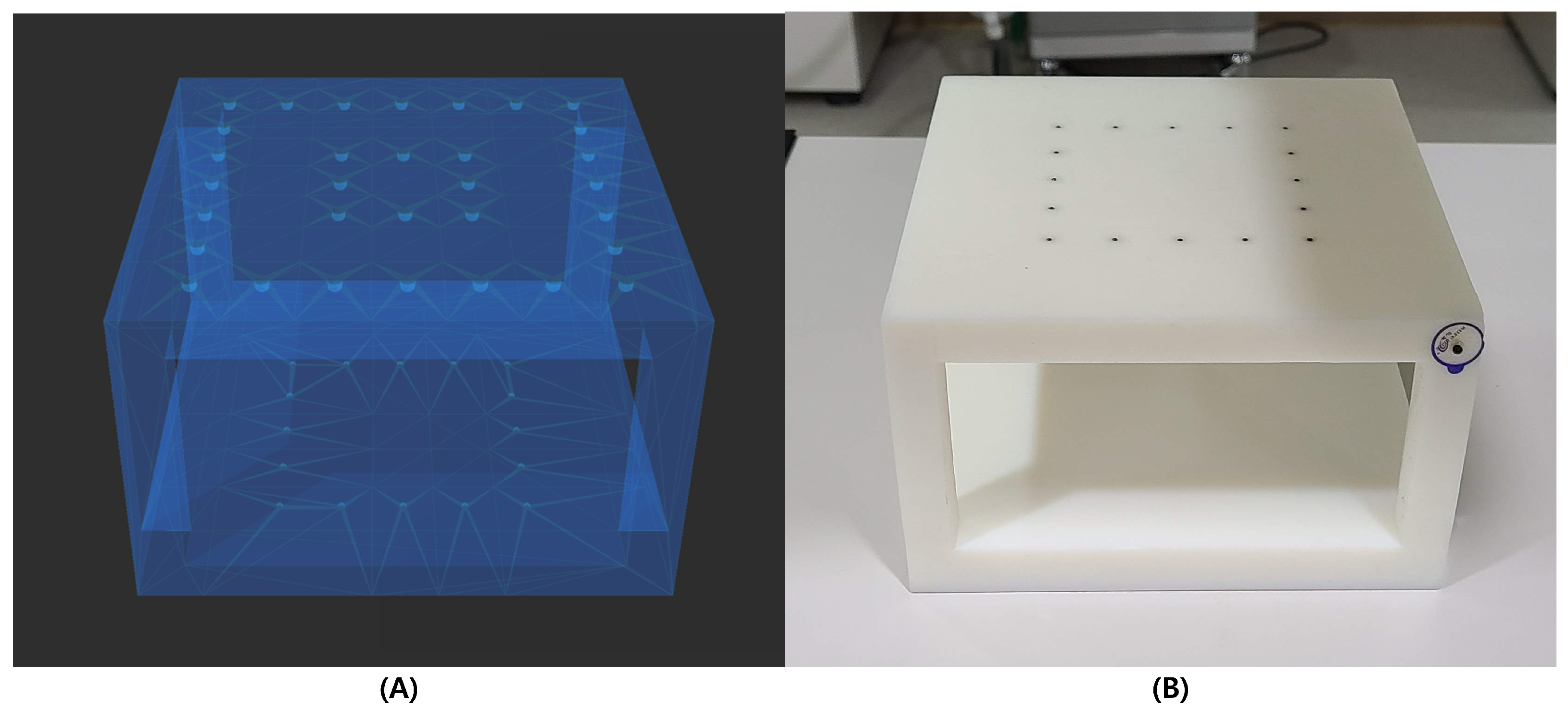
This study aims to develop a projectional geometry calibration method for radiographic use, which is essential for performing registration between 2D radiographic images and CBCT data acquired intraoperatively during an image-guided angiographic intervention. The clinical target of this study is a C-arm angiographic imaging device that has been used in vascular intervention procedures and is equipped with CBCT imaging capabilities. While operating the CBCT, this device can provide sinogram data and radiographic image data with multi-directional projection images at various angles, which are then used to reconstruct 3D CT volume data. The significance of this study is in the calculation and application of the geometric parameters of radiographs required for image-guided vascular intervention procedures using the sinogram data obtained during CBCT acquisition in the intervention room. Herein, we aim to improve the accuracy of the calibration method using sinogram data acquired during the interventional procedures without any additional radiation exposure and any significant increase in the computational time. We attempted to obtain robust calibration accuracy along various orientations of the X-ray gantry using sinogram data and only one calibration procedure. Furthermore, we did not want to permanently fix any calibration pattern to obtain a clear object without using any additional calibration markers. A calibration phantom with ball bearings to establish accurate 3D locations was designed for this purpose, and is used before surgery to calibrate the geometry of the X-ray imaging device. This study also focused on executing the calibration method in under a minute, which is an acceptable calculation time for image-induced vascular intervention, and within a 1 mm accuracy.

2. Materials Furthermore, Methods

2.1. Phantom Design Furthermore, Fabrication

The calibration phantom used a 2-layered model designed with 3D CAD software, SolidWorks (Dassault Systèms SolidWorks Corp., Vélizy-Villacoublay, France), and was built with plastic material, Vero (Stratasys, Rehovot, Israel), using a 3D printer, Objet30 Prime (Stratasys, Rehovot, Israel). Figure 1 shows the CAD model of the calibration phantom and the manufactured phantom, both of which have fiducial markers to establish precise 3D locations. Figure 2 depicts the layouts of the two layers. The size of the phantom is 170 mm × 170 mm × 103.54 mm, and lead ball bearings, SL-20 and SL-40 (Suremark, Simi Valley, CA, USA) lead, were used as fiducial markers. The upper and lower layers are the same size but differ in height. On the upper layer, 16 markers with a diameter of 2 mm are arranged in a rectangular pattern at 20 mm intervals toward the X-ray source. On the lower layer, there are two sizes of markers—eight 4 mm diameter markers arranged in small rectangular shapes at 20 mm intervals and twenty-four 4 mm diameter markers arranged in large rectangular shapes at 20 mm intervals and located toward the X-ray detector. Only the height differs between the horizontal and vertical centers of the three squares and the center of the phantom.

2.2. Definition of the Coordinate System

Figure 3 depicts the coordinate system defined for imaging device calibration. The origin of the world coordinate system is defined as being in the center of the detector, and the X-ray source is aligned with the z-axis of the system. This means that the x and y of the centers of the X-ray source and detector are the same and have different heights (z coordinate), a choice that avoids computational complexity and burden. The CT system rotates in the y-axis direction about the rotational center, which is commonly referred to as the isocenter.

Equation (1) defines the position of the upper and lower layers in the calibration phantom, position of the X-ray source, center of the X-ray detector, and isocenter in the world coordinate system. These represent the 3D information regarding the imaging device. The center of the X-ray detector is the origin of the world coordinate system.

$$\begin{array}{cc}\hfill P^u& =(P_x^u,P_y^u,P_z^u):\mathrm{Upper}\mathrm{of}\mathrm{Phantom}\hfill \\ \hfill P^l& =(P_x^l,P_y^l,P_z^l):\mathrm{Lower}\mathrm{of}\mathrm{Phantom}\hfill \\ \hfill S& =(S_x,S_y,S_z):\mathrm{Position}\mathrm{of}\mathrm{X}-\mathrm{ray}\mathrm{Source}\hfill \\ \hfill D& =(D_x,D_y,D_z)=(0,0,0):\mathrm{Center}\mathrm{of}\mathrm{X}-\mathrm{ray}\mathrm{Detector}\hfill \\ \hfill I& =(I_x,I_y,I_z):\mathrm{Isocenter}\hfill \end{array}$$

(1)

Equation (2) presents the coordinates of the projected point on the upper and lower layers of the phantom, which give the 2D information in the X-ray image.

$$\begin{array}{cc}\hfill {P^{\prime }}^u& =({P^{\prime }}_x^u,{P^{\prime }}_y^u,{P^{\prime }}_z^u)\hfill \\ \hfill {P^{\prime }}^l& =({P^{\prime }}_x^l,{P^{\prime }}_y^l,{P^{\prime }}_z^l)\hfill \end{array}$$

(2)

where, ${P^{\prime }}_z^u={P^{\prime }}_z^l=D_z=0$

2.3. Detection of Fiducial Markers

The sinogram is in the form of stacked data of the projection images at various angles. The fiducial markers in the images were detected at each angle, and the detected markers were divided into upper and lower layer markers. Since the X-ray attenuation coefficient in the fiducial marker is much higher than in the plastic material of the phantom, the fiducial markers could be distinguished using the threshold-based segmentation method [12]. Therefore, by applying the threshold value to the CT sinogram data, the markers could be segmented, and the layer to which the fiducials belonged could be classified. Then the centers of markers were determined by successively applying the Hough circle transformation [13] and findContours function [14] of the OpenCV library. Since the upper and lower fiducial markers have different heights and radii, they could be divided into two groups based on the sizes of the detected markers.

Since some markers (close to each other or superimposed) could not be detected well, a detection algorithm that considers these cases is developed. The detected markers were divided into four sections—top, bottom, left, and right—and a rectangle was formed using the detected markers. Four straight lines were drawn connecting both corner points for each divided section. The corners of the detection rectangle were formed by the four intersection points of the four lines. Consequently, even if a few markers are missed during the detection process, a consistent rectangle can be generated using the detected markers.

Calibration is performed as shown in Figure 4 based on the position of the marker detected in the sinogram data.

2.4. Calculation of SDD, Phantom, Source, and Detector Position

The projectional radiography of the phantom is magnified based on the ratio between X-ray source-to-phantom distance and the source-to-detector distance (SDD). Equation (3) uses a triangular shape to express a proportional equation in which a point on the phantom is projected–expanded.

$$\begin{array}{c}\hfill S_z-D_z:S_z-P_z=P_z^{\prime }:P_x\end{array}$$

(3)

By defining $S_z-P_z$ as the parameter $z^{\prime }$, Equation (3) can be expressed as Equation (4).

$$S_z:z^{\prime }=P_z^{\prime }:P_x$$

(4)

where, $z^{\prime }=S_z-P_z$

When projected to the x–z plane, the system can be expressed as shown in Figure 5. Equation (5) expresses the coordinates of each point in Figure 5.

$$\begin{array}{cc}\hfill P^{u,M}=& [P_x^M,P_z^M]\hfill \\ \hfill P^{u,L}=& [P_x^M+W^{u}cos{\theta }_y,P_z^M-W^{u}sin{\theta }_y]\hfill \\ \hfill P^{u,R}=& [P_x^M+W^{u}cos{\theta }_y,P_z^M+W^{u}sin{\theta }_y]\hfill \\ \hfill P^{l,L}=& [P_x^M+Hsin{\theta }_y-W^{l}cos{\theta }_y,P_z^M-Hcos{\theta }_y-W^{l}sin{\theta }_y]\hfill \\ \hfill P^{l,R}=& [P_x^M+Hsin{\theta }_y+W^{l}cos{\theta }_y,P_z^M-Hcos{\theta }_y+W^{l}sin{\theta }_y]\hfill \end{array}$$

(5)

where,

• L, R, and M represent the left, right, and middle point in the 2D projection system, respectively.
• W and H represent the width and height of the phantom, respectively.

Equations (4) and (5) can be substituted and summarized as Equation (6).

$$\begin{array}{cc}\hfill sin{\theta }_y=& \frac{{P^{\prime }}_x^{u,L}+{P^{\prime }}_x^{u,R}-2{P^{\prime }}_x^{u,M}}{W^u·({P^{\prime }}_x^{u,L}-{P^{\prime }}_x^{u,R})}·z^{\prime }\hfill \\ \hfill cos{\theta }_y=& \frac{{P^{\prime }}_x^{l,R}-{P^{\prime }}_x^{l,L}-\frac{sin{\theta }_y}{z^{\prime }}·W^l({P^{\prime }}_x^{l,L}+{P^{\prime }}_x^{l,R})}{H({P^{\prime }}_x^{l,L}-{P^{\prime }}_x^{l,R})+2S_z·W^l}·z^{\prime }\hfill \end{array}$$

(6)

Since ${sin{\theta }_y}^2+{cos{\theta }_y}^2=1$, the x- and z-coordinates of the phantom and SDD can be calculated by Equation (7).

$$\begin{array}{cc}\hfill S_z=& \frac{{P^{\prime }}_x^{u,M}-{P^{\prime }}_x^{u,L}·(W^u·a+1)}{W^u·b}\hfill \\ \hfill P_z^{u,M}=& S_z-z^{\prime }=S_z-\sqrt{{(a^2+b^2)}^{-1}}\hfill \\ \hfill P_x^{u,M}=& \frac{a}{S_z}{z}^{\prime }\hfill \end{array}$$

(7)

where, $a=\frac{{P^{\prime }}_x^{u,L}+{P^{\prime }}_x^{u,R}-2{P^{\prime }}_x^{u,M}}{W^u·({P^{\prime }}_x^{u,L}-{P^{\prime }}_x^{u,R})},b=\frac{{P^{\prime }}_x^{l,R}-{P^{\prime }}_x^{l,L}-a·W^l({P^{\prime }}_x^{l,L}+{P^{\prime }}_x^{l,R})}{H({P^{\prime }}_x^{l,L}-{P^{\prime }}_x^{l,R})+2S_z·W^l}$

To calculate the 3D initial coordinates of the phantom and the source, the same process from Equations (3)–(7) is performed for the system projected to the y–z plane.

2.5. Calculation of Isocenter Position

The SVD method was used to calculate the 3D coordinates of the phantom and the isocenter [10,11]. The positions of known markers are defined with respect to the coordinates of the phantom. Therefore, a relational equation should be established by considering the initial position and orientation with respect to the current coordinates of the markers. Furthermore, the rotational angle about the z-axis, ${\theta }_z$, can be calculated using the minAreaRect function [15] of the OpenCV library. A 4 × 4 homogeneous transformation matrix can be expressed as the relational Equation (8) of a point rotated along the X- and Y-axes.

$$\begin{array}{c}\hfill P^r=M·P=T{R}_x{R}_y{T}^{-1}P\\ \hfill \left[\begin{array}{c}{P}_x^r\\ P_y^r\\ P_z^r\\ 1\end{array}\right]=\\ \hfill \left[\begin{array}{cccc}1& 0& 0& I_x\\ 0& 1& 0& I_y\\ 0& 0& 0& I_z\\ 0& 0& 0& 1\end{array}\right]\left[\begin{array}{cccc}1& 0& 0& 0\\ 0& cos{\theta }_x& -sin{\theta }_x& 0\\ 0& sin{\theta }_x& cos{\theta }_x& 0\\ 0& 0& 0& 1\end{array}\right]\left[\begin{array}{cccc}cos{\theta }_y& 0& sin{\theta }_y& 0\\ 0& 1& 0& 0\\ -sin{\theta }_y& 0& cos{\theta }_y& 0\\ 0& 0& 0& 1\end{array}\right]\left[\begin{array}{cccc}1& 0& 0& -I_x\\ 0& 1& 0& -I_y\\ 0& 0& 0& -I_z\\ 0& 0& 0& 1\end{array}\right]\left[\begin{array}{c}{P}_x\\ P_y\\ P_z\\ 1\end{array}\right]\end{array}$$

(8)

The proportional expression between $P^r$ and the projected point $P^{\prime }$ is given by Equation (9).

$$\begin{array}{c}\hfill S_z:S_z-P_z^r=P_x^{\prime }:P_x^r\\ \hfill S_z:S_z-P_z^r=P_y^{\prime }:P_y^r\end{array}$$

(9)

Equations (8) and (9) can be substituted and summarized into Equation (10).

$$\begin{array}{cc}\hfill P_x^{\prime }·S_z=& P_x[S_{z}cos{\theta }_y-P_x^{\prime }sin{\theta }_{y}cos{\theta }_x]+P_y\left[P_x^{\prime }sin{\theta }_x\right]\hfill \\ \hfill & +P_z[S_{z}sin{\theta }_y+P_x^{\prime }cos{\theta }_{y}cos{\theta }_x]+I_x[S_z(1-cos{\theta }_y)+P_x^{\prime }sin{\theta }_{y}cos{\theta }_x]\hfill \\ \hfill & -I_y\left[P_x^{\prime }sin{\theta }_x\right]+I_z[P_x^{\prime }(1-cos{\theta }_{y}cos{\theta }_x)-S_{z}sin{\theta }_y]\hfill \\ \hfill P_y^{\prime }·S_z=& P_x[S_{z}sin{\theta }_{y}sin{\theta }_x-P_y^{\prime }sin{\theta }_{y}cos{\theta }_x]+P_y[S_{z}cos{\theta }_x+P_y^{\prime }sin{\theta }_x]\hfill \\ \hfill & +P_z[P_y^{\prime }cos{\theta }_{y}cos{\theta }_x-S_{z}cos{\theta }_{y}sin{\theta }_x]+I_x[P_y^{\prime }sin{\theta }_{y}cos{\theta }_x-S_{z}sin{\theta }_{y}sin{\theta }_x]\hfill \\ \hfill & -I_y[S_z(1-cos{\theta }_x)-P_y^{\prime }sin{\theta }_x]+I_z[S_{z}cos{\theta }_{y}sin{\theta }_x+P_y^{\prime }(1-cos{\theta }_{y}cos{\theta }_x)]\hfill \end{array}$$

(10)

The least-squares solution can be calculated by defining a matrix form of $Ax=b$ using SVD [10,11]. Therefore, Equation (10) can be converted into Equation (11) in the form of $Ax=b$.

$$\begin{array}{c}\hfill {\left[\begin{array}{ccc}{S}_{z}cos{\theta }_y-P_x^{\prime }sin{\theta }_{y}cos{\theta }_x& \cdots & P_x^{\prime }(1-cos{\theta }_{y}cos{\theta }_x)-S_{z}sin{\theta }_y\\ S_{z}sin{\theta }_{y}sin{\theta }_x-P_y^{\prime }sin{\theta }_{y}cos{\theta }_x& \cdots & S_{z}cos{\theta }_{y}sin{\theta }_x+P_y^{\prime }(1-cos{\theta }_{y}cos{\theta }_x)\end{array}\right]}^T\left[\begin{array}{c}{P}_x\\ P_y\\ P_z\\ I_x\\ I_y\\ I_z\end{array}\right]\\ \hfill =\left[\begin{array}{c}{P}_x^{\prime }·S_z\\ P_y^{\prime }·S_z\end{array}\right]\end{array}$$

(11)

Since Equation (11) is a matrix of one angle, the matrix of several angles can be expressed as Equation (12).

$$\begin{array}{c}\hfill {\left[\begin{array}{ccc}{S}_{z}cos{\theta }_{y,0}-P_x^{\prime }sin{\theta }_{y,0}cos{\theta }_{x,0}& \cdots & P_x^{\prime }(1-cos{\theta }_{y,0}cos{\theta }_{x,0})-S_{z}sin{\theta }_{y,0}\\ S_{z}sin{\theta }_{y,0}sin{\theta }_{x,0}-P_y^{\prime }sin{\theta }_{y,0}cos{\theta }_{x,0}& \cdots & S_{z}cos{\theta }_{y,0}sin{\theta }_{x,0}+P_y^{\prime }(1-cos{\theta }_{y,0}cos{\theta }_{x,0})\\ ⋮& ⋮& ⋮\end{array}\right]}^T\left[\begin{array}{c}{P}_x\\ P_y\\ P_z\\ I_x\\ I_y\\ I_z\end{array}\right]\\ \hfill =\left[\begin{array}{c}{P}_{x,0}^{\prime }·S_z\\ P_{y,0}^{\prime }·S_z\\ ⋮\end{array}\right]\end{array}$$

(12)

Equation (12) obtains the $Ax=b$ matrix in which $P_x,P_y,P_z,I_x,I_y,I_z$ become variables. Matrix A can be decomposed into $A=U\Sigma V^T$ by the SVD theorem.

$$\begin{array}{cc}\hfill & A:m\times n\mathrm{rectangular}\mathrm{matrix}\hfill \\ \hfill & U:m\times m\mathrm{orthogonal}\mathrm{matrix}\hfill \\ \hfill & \Sigma :m\times n\mathrm{diagonal}\mathrm{matrix}\hfill \\ \hfill & V:m\times m\mathrm{orthogonal}\mathrm{matrix}\hfill \end{array}$$

The pseudo-inverse of A is calculated as $A^{+}=V{\Sigma }^{+}{U}^T$. Therefore, in $Ax=b$, the x can be calculated as $x=A^{+}b$, and the calculation is the least-squares solution that minimizes $∥Ax-b∥$. Consequently, the least-squares solution of Equation (12) can be expressed as Equation (13).

$$\begin{array}{cc}\hfill x=& A^{+}b\hfill \\ \hfill =& {\left[\begin{array}{cccccc}{P}_x& P_y& P_z& I_x& I_y& I_z\end{array}\right]}^T\hfill \end{array}$$

(13)

Since the eight corners detected from the phantom are used, Equation (13) is expanded to Equation (14) to calculate the coordinates of the eight corners.

$$\begin{array}{cc}\hfill x=& A^{+}b\hfill \\ \hfill =& {\left[\begin{array}{cccccccccc}{P}_{x,0}& P_{y,0}& P_{z,0}& \cdots & P_{x,7}& P_{y,7}& P_{z,7}& I_x& I_y& I_z\end{array}\right]}^T\hfill \end{array}$$

(14)

2.6. Evaluation

The projections of the fiducial markers to the detector are computed and compared with the locations of the fiducials in the sinogram corresponding to the angular orientation of the X-ray gantry based on the geometric parameters obtained using the calibration method.

Equation (3) can be used to express the projection result. Equation (15) shows the error between the coordinates predicted by the geometric parameters and the locations detected in the same angle image of the sinogram data.

$$\begin{array}{cc}\hfill E_{x_{\theta }}=& {P^{\prime }}_{x,\theta }^d-{P^{\prime }}_{x,\theta }\hfill \\ \hfill E_{y_{\theta }}=& {P^{\prime }}_{y,\theta }^d-{P^{\prime }}_{y,\theta }\hfill \\ \hfill E_{\theta }=& \sqrt{E_{x_{\theta }}^2+E_{y_{\theta }}^2}\hfill \end{array}$$

(15)

where, ${P^{\prime }}_{x,\theta }^d\mathrm{and}{P^{\prime }}_{y,\theta }^d\mathrm{are}\mathrm{the}\mathrm{marker}\mathrm{positions}\mathrm{detected}\mathrm{in}\mathrm{the}\mathrm{angle}\theta$ image of the sinogram data.

3. Experiments

3.1. Experimental Setup

The Artis zee floor system is a C-arm angio imaging device with a 2D projectional X-ray fluoroscopic imaging function and a CBCT imaging function that was used in the experiment (Siemens AG, Munich, Germany). The Daegu-Gyeongbuk Medical Innovation Foundation has established the imaging system (KMEDIhub, Daegu, Republic of Korea). Figure 6 depicts the imaging room where the experiments were conducted. The phantom experiment was also conducted in the imaging room. The computer used in the experiments is equipped with an Intel i7 9700KF CPU, 40GB of DDR4 RAM, and an NVIDIA GeForce RTX 3080 GPU.

3.2. Software Implementation of the Geometric Calibration for X-ray Imaging

C++ and the MFC library were used to create the software application for geometric calibration for X-ray imaging. Figure 7 shows the graphical user interface (GUI) for the application. VTK 8.2.0, GDCM 2.8.9, and OpenCV 4.0.1 open-source libraries were used to implement the core functions. Each function, as well as the order in which it was used, is described below. The ‘Load DICOM’ button reads the sinogram data and X-ray images, as well as their metadata, such as the angle of each slice and pixel spacing. A selected slice of data of the sinogram data is rendered in ‘Window 1’. The rendered slice in ‘Window 1’ can be changed to a different slice with a different angle using either the mouse or keyboard. The ‘Calibration’ button enables the calculation of the geometric parameters of the X-ray imaging using the loaded sinogram data belonging to the predefined range of angles (in degrees) and angle interval. The angle range and interval can also be defined using the application GUI’s edit boxes. The calculated geometric parameters are displayed in the annotation at the top right of ‘Window 1’ and saved as an XML file. The ‘Projection Error’ check box allows the user to specify whether the error of ‘Window 2’ is displayed. The ‘2D Reflection Button’ allows the operator to overlay two images in the same view. In ‘Window 2’, the computational result of the projected markers based on the geometric parameters and the detected markers in the corresponding slice of sinogram data can be superimposed. Additionally, the ‘Error’ button calculates the root mean square error between the superimposed data in ‘Window 2’, and the error is also written to the file in CSV format. For comparison purposes, previously computed results are also loadable using the ‘Read Points’ button, which enables the reading of the computed positions of the projected markers written in the XML file format.

3.3. Data Acquisition

The imaging device was used for the experiments, and the image data were acquired in DICOM file format, which is commonly used in medical applications. After securely positioning the calibration phantom on the table, CBCT data were collected, and the sinogram and reconstructed volume were saved to files. Following that, several 2D X-ray fluoroscopic images were captured at various X-ray gantry orientations. The metadata that contains the detailed information of the image data is stored with the image data for calibration. The dimensions of X-ray fluoroscopic image data are 2480 × 1920, and the spacings of the x- and y-direction are 0.154 mm and 0.154 mm, respectively. This information is stored in the tags (0018, 1604), (0018, 1608), and (0018, 1164) of the metadata. The sinogram data are a stack of 469 images with a dimension of 1240 × 960, and the dimension is stored in the same tags (0018, 1604) and (0018, 1608) as the X-ray data, and the number of images is stored in the tag (0028, 0008). Since the device that acquired the X-ray data and sinogram data is the same, the spacing of the pixels for the sinogram data is twice that of the spacing for the X-ray data. Each projectional image for the sinogram was acquired every 0.399 degrees, from −98.95 degrees to 99.04 degrees, and the angle information is stored in the metadata tags (0018, 1520). The geometric calibration was applied to 301 images ranging from −60.12 degrees to 59.85 degrees for the experiment.

4. Results

In the experiments, ten parameters were computed for the geometrical calibration of X-ray projectional imaging, including the SDD, position and orientation of the phantom, and position of the isocenter. The sinogram and 2D projectional X-ray images were obtained, and the evaluation procedures were followed using the software application developed in this study.

Three different methods were used to analyze the results. First, the accuracy of the calibration method was assessed using the angular range of the sinogram data used in the calibration. As shown in Figure 8, the calibration algorithm was executed under a variety of data size conditions, with the data set ranging from −15 to 15 to −60 to 60, increasing 10 degrees at each step. The results are presented in the orange bar graph of Figure 8, which shows that the operation with a wide range of data provided improved accuracy. If the data are wider than the angle from −40 to 40, the accuracy of the calibration was stable, and further improvement could not be detected. However, as the range of the data increased, so did the computational time for the calibration algorithm, as shown in the blue plot in Figure 8.

Second, the accuracy of the calibration method was assessed using the data intervals applied to the calibration algorithm. The calibration method was followed in several conditions with different angle intervals but with the same angular range applied to the algorithm, as shown in Figure 9. As illustrated with the orange bar graph in Figure 9, the narrower the angular interval, the smaller the error. The improvement in the error was not dramatic but gradual. Furthermore, as the angular interval widened, the calculation time decreased, which is indicated by the blue plot in Figure 9.

We also tested the robustness of our method by projecting the 3D positions of the fiducial markers into various angles based on the rotation of the C-arm gantry and calculating the mean error between the projected fiducial positions and the centers of the fiducial markers in the sinogram projection image. Calibrations were performed under five different conditions, as shown in Figure 10, with angular ranges ranging from −20 to 20 degrees, −30 to 30 degrees, −40 to 40 degrees, −50 to 50 degrees, and −60 to 60 degrees. Based on the results of each trial with different conditions, the 3D fiducial positions were projected into all of the projected images that belong to the sinogram. As illustrated in Figure 10, the evaluation result of the calibration with sinogram data with a range of −20 to 20 degrees shows the worst accuracy. The accuracy improved by broadening the data range used by the calibration algorithm. Furthermore, as the angle moved away from 0 degrees, the projectional errors in each trial increased, and the gradient became much larger in the rotation angle outside of the range of the data used for calibration. In addition, the wider the angle range, the better the accuracy of the projectional error. Moreover, the gradient is much less for the results with a narrower data range.

5. Discussion

We conducted phantom experiments and analyzed the experimental results using three different methods to evaluate our calibration method. First, we assessed the accuracy of the calibration method using a variety of data range conditions applied to the calibration algorithm. Calibrations were performed using different ranges of sinogram data, and the results are shown in Figure 8. The results show that a wider range of sinogram angles could guarantee improved accuracy compared to a narrower range of data or a single image from one angle. Although a broader range of data yields higher accuracy, it also necessitates more computational time. As shown in the blue plot of Figure 8, by increasing the range of the data, the computational time also increases significantly. However, the accuracy with different data ranges shows that there are no significant differences in accuracy if the data range is wider than −40 to 40 degrees. Therefore, when considering the required computational time, the range between −40 and 40 degrees is an optimized range of data for calibration.

Second, we assessed how much the data interval affected the accuracy. The calibration algorithm’s accuracy was tested with intervals ranging from 0.4 degrees to 3.2 degrees over the same angular range. Figure 9 depicts the evaluation results, which show that the interval of the sinogram data applied to the algorithm affects the accuracy less than the range of the sinogram data. As shown in Figure 9, the results show no trend of decreasing accuracy as the data interval is increased. The computational time, on the other hand, can be reduced by reducing the amount of data and increasing the interval of the data using the same angular range. Although the data size is reduced linearly by increasing the interval of the data linearly, the computational time is not reduced linearly. This is because the data loading time is involved in the computational time. By reducing the data size (by increasing the interval), the percentage of the loading time relative to the entire computational time is increased. Consequently, the computational time can be reduced by selecting a larger interval, as shown in Figure 9. Given the accuracy and computational time constraints, an interval of 1.6 degrees can be considered an optimized interval for the data used by the calibration algorithm.

Finally, the robustness of the algorithm was evaluated based on the results with various data ranges by projecting 3D fiducial markers of the phantom to each projectional image of the sinogram and comparing the error between the projected coordinates and the center of the fiducial marker region in each image slice of the sinogram. As shown in Figure 10, the condition that applies a wider range of sinogram data to the algorithm outperforms that with a narrower range. Furthermore, the shape of the plot is similar to the parabolic shape of the quadratic polynomial with a minimum value near 0, and errors increase as the rotation angle of the C-arm gantry increases in both directions within the range. The accuracy of the calibration presented errors below 1 mm within the method’s range, whereas the errors are much larger outside of the range, particularly for the ranges of −20 to 20 degrees and −30 to 30 degrees. For the wider range of −40 to 40 degrees, the overall accuracy is below 1 mm. The plots in Figure 10 are asymmetric due to the rotational error of the C-arm gantry. If the rotational motion of the C-arm gantry is pure, the error would demonstrate a symmetric pattern. However, since the rotational motion has some errors during the rotational operation of the C-arm gantry in a real situation, due to the vibration or bias of the rotational center of the C-arm, the error pattern is not perfectly symmetric.

6. Conclusions Furthermore, Future Work

This study aims to create a calibration method that can be used in the intervention theater immediately prior to a vascular intervention procedure. Furthermore, it aims to improve the accuracy of the calibration method using sinogram data acquired during the CBCT imaging process. In other words, the goal of this study is to create a calibration method that ensures the safety of the vascular intervention procedure and executes within the acceptable computational time for the image-guided vascular intervention room without exposing the patient to any additional radiation.

The proposed method is a phantom-based calibration technique that uses sinogram data to compute ten geometric parameters of the imaging device. By comparing and evaluating the calibration accuracy across various angular ranges and interval conditions, the optimal angle range and interval are proposed. Consequently, the optimal calibration conditions considering the calculation time and accuracy were found to be an angular range from −40 to 40 degrees, with an optimal angular interval of 1.6 degrees. Therefore, a calibration method with an operation time of 2.92 s and a mean error of 0.36 mm could be achieved, thus satisfying our goal of below 1 mm accuracy within a minute computational time. We plan to conduct additional research in the near future to apply this calibration method to a robotic system for vascular intervention.

References

1. Peters, T.M. Image-guidance for surgical procedures. Phys. Med. Biol. 2006, 51, 505–540. [Google Scholar] [CrossRef] [PubMed]
2. Kohan, D.; Jethanamest, D. Image-guided surgical navigation in otology. Laryngoscope 2012, 122, 2291–2299. [Google Scholar] [CrossRef] [PubMed]
3. Song, H.S.; Woo, J.H.; Won, J.Y.; Yi, B.J. In Vivo Usability Test of Vascular Intervention Robotic System Controlled by Two Types of Master Devices. Appl. Sci. 2021, 11, 5453. [Google Scholar] [CrossRef]
4. Sato, K.; Ohnishi, T.; Sekine, M.; Haneishi, H. Geometry calibration between X-ray source and detector for tomosynthesis with a portable X-ray system. Int. J. Comput. Assist. Radiol. Surg. 2017, 12, 707–717. [Google Scholar] [CrossRef] [PubMed] [Green Version]
5. Ford, J.C.; Zheng, D.; Williamson, J.F. Estimation of CT cone-beam geometry using a novel method insensitive to phantom fabrication inaccuracy: Implications for isocenter localization accuracy. Med. Phys. 2011, 38, 2829–2840. [Google Scholar] [CrossRef] [PubMed] [Green Version]
6. Miao, H.; Wu, X.; Zhao, H.; Liu, H. A phantom-based calibration method for digital x-ray tomosynthesis. J. X-ray Sci. Technol. 2012, 20, 17–29. [Google Scholar] [CrossRef] [PubMed]
7. Nguyen, V.; Beenhouwer, J.D.; Sanctorum, J.G.; Wassenbergh, S.V.; Bazrafkan, S.; Dirckx, J.J.J.; Sijbers, J. A low-cost geometry calibration procedure for a modular cone-beam X-ray CT system. Nondestruct. Test. Eval. 2020, 35, 252–265. [Google Scholar] [CrossRef]
8. Fragnaud, C.; Remacha, C.; Betancur, J.; Roux, S. CAD-based X-ray CT calibration and error compensation. Meas. Sci. Technol. 2022, 33, 065024. [Google Scholar] [CrossRef]
9. da Silva, J.; Chen, M.; Eriksson, M. A paddle-wheel phantom for geometric calibration of cone-beam CT with offset detector. SPIE Med. Imageing 2022, 12031, 1203120. [Google Scholar]
10. Golub, G.; Kahan, W. Calculating the Singular Values and Pseudo-Inverse of a Matrix. J. Soc. Ind. Appl. Math. Ser. B Numer. Anal. 1965, 2, 205–224. [Google Scholar] [CrossRef]
11. Akritas, A.G.; Malaschonok, G.I. Applications of singular-value decomposition (SVD). Math. Comput. Simul. 2004, 67, 15–31. [Google Scholar] [CrossRef]
12. Fu, K.S.; Mui, J.K. A survey on image segmentation. Pattern Recognit. 1981, 13, 3–16. [Google Scholar] [CrossRef]
13. Ballard, D.H. Generalizing the Hough transform to detect arbitrary shapes. Pattern Recognit. 1980, 13, 111–122. [Google Scholar] [CrossRef] [Green Version]
14. Suzuki, S.; Abe, K. Topological structural analysis of digitized binary images by border following. Comput. Vis. Graph. Image Process. 1985, 30, 32–46. [Google Scholar] [CrossRef]
15. Freeman, H.; Shapira, R. Determining the minimum-area encasing rectangle for an arbitrary closed curve. Commun. ACM 1975, 18, 409–413. [Google Scholar] [CrossRef]
Figure 1. Calibration phantom model (A) was designed using CAD software, and the phantom (B) was built with a 3D printer, with lead-bearing fiducial markers to establish precise locations.
Applsci 12 07543 g001
Figure 2. Two-dimensional drawings of the top and bottom layers of the phantom. The brackets represent the 3D coordinates of the center of each ball bearing, in mm. (A) is the lower layer with 2 mm diameter ball bearings, and (B) is the upper layer with 4 mm ball bearings.
Applsci 12 07543 g002
Figure 3. Coordinate system used in the calibration; the red axes show the world coordinate system, and the blue axes represent the orientation of the phantom.
Applsci 12 07543 g003
Figure 4. A flowchart of the calibration method.
Applsci 12 07543 g004
Figure 5. System projected in two dimensions in the y-axis direction.
Applsci 12 07543 g005
Figure 6. C-arm angio imaging device was applied to the experiment, which has the functions of 2D projectional X-ray imaging and CBCT imaging.
Applsci 12 07543 g006
Figure 7. Software application for the geometric calibration of X-ray imaging was implemented, which provides core functions for the calibration and graphical user interface.
Applsci 12 07543 g007
Figure 8. Graph of mean errors (orange bars) and computational time (blue plot) according to different angular ranges applied to the calibration algorithm; the interval of the data is 0.4 degrees for each range. The x-axis represents the angular range of the data applied to the calibration. The y-axis on the left and right give the error and computational time, respectively.
Applsci 12 07543 g008
Figure 9. Graph of mean errors (orange bars) and computational time (blue plot) according to the different angular intervals applied to the calibration algorithm with the same range of the applied data; the angular interval ranges from 0.4 degrees to 3.2 degrees; the x-axis represents the angular interval of the image used in the calculation. The y-axis on the left gives the error, and that on the right gives the computational time.
Applsci 12 07543 g009
Figure 10. Graph of the projection mean errors according to the angle range with an angle interval of 0.4 degrees; the x-axis represents the rotation angle of each slice in the sinogram, and the y-axis represents the projection mean error of the eight corner points [mm].
Applsci 12 07543 g010
Publisher’s Note: MDPI stays neutral with regard to jurisdictional claims in published maps and institutional affiliations.