Distribution of Magnetic Flux Density under Stress and Its Application in Nondestructive Testing

Abstract

Carbon steels are commonly used in railroad, shipment, building, and bridge construction. They provide excellent ductility and toughness when exposed to external stresses. They are able to resist stresses and strains effectively, and guarantee safe operation of the devices through nondestructive testing (NDT). The magnetic metal memory (MMM) can be used as an NDT method to measure the residual stress. The ability of carbon steel to produce a magnetic memory effect under stress is explored here, and enables the magnetic flux density to be analyzed. The relationship between stress and magnetic flux density has not been fully presented until now. The purpose of this paper is to assess the relationship between stress distribution and the magnetic flux density measured by the experiment. For this, an experimental method for examining a carbon steel plate (SA 106), based on the four-point loading test, was used. The effect of stresses resulting from the applied loads on the response of the experimented SA 106 specimen was examined. A three directional tunnel magnetoresistance (TMR) measurement system was used to collect the triaxial magnetic flux density distribution in the SA 106 specimen. In addition, finite element method (FEM) analyses were performed, and provided information on the direction and distribution of the stress over the studied SA 106 specimen. Indeed, a correlation was derived by comparing the stress analysis by FEM and the measured triaxial magnetic flux density.

1. Introduction

Carbon steels are broadly used in the railroad, shipment, and building industries. They are designed with a specific chemical composition for each of these sectors, and they offer ductility and toughness when exposed to external stresses. They are able to provide effective resistance to stress and strain, and ensure the safe operation of equipment.

The presence of even a tiny amount of heterogeneity formed during the process of manufacturing and operating the material can alter its mechanical properties, and endanger the performance and safety of the structure or part, and can arise unexpectedly without prior prevention. To this end, it is necessary to regularly inspect the infrastructure with the appropriate nondestructive testing (NDT) techniques to identify defects and prevent any type of failure [1,2,3,4,5,6,7,8,9,10]. Multiple nondestructive testing techniques, such as magnetic particle testing (MPT), liquid penetrant testing (PT), eddy current testing (ECT), magnetic Barkhausen emission (MBE), magneto-acoustic emission (MAE), magnetic flux leakage (MFL), etc., can be used for this purpose [11,12,13,14,15,16]. However, when it comes to early failure detection, including stress concentration detection and ferromagnetic material fatigue damage, the metal magnetic memory (MMM) method is often used instead of the conventional NDT methods [17,18,19]. This approach is novel for the nondestructive testing of ferromagnetic devices, and is actually based on the residual magnetization measurement, which occurs in the given material under the action of a stress load or external fields [20,21]. The MMM testing technique was initially put forward by Dubov in 1997. This technology is not limited to the previously mentioned uses, and also allows the evaluation of deficiencies in ferromagnetic structures, including the detection of the position of the defect, microcracking, welded joints at the production stage, plastic deformation, etc. [22,23]. Moreover, the MMM method offers distinctive features; among which, the simplicity of the operating principle, the low cost of the measuring equipment, the need for no external sources of the magnetic field, and no treatment of the surface of the structures nor the premagnetization or demagnetization of the target specimens [5,24,25,26].

Over the past twenty-five years, the MMM and its application to the investigation of defects in ferromagnetic structures is among the nondestructive magnetic testing methods that have attracted considerable interest from many researchers around the world [4,27,28,29,30,31,32]. Leng et al. [33] and Huang et al. [30] performed fatigue bending experiments under various stress levels to study the magnetomechanical effect. The results reveal that the metal magnetic memory signal can be utilized to assess the damage degree of materials in the elastic and plastic deformation phases, and the degree of stress concentration. Shi et al. [34] conducted a tension–tension fatigue test of ferromagnetic steel with different stress concentration factors, and they concluded that the stress concentration factor has a significant impact on the variation of magnetic signals in a dynamic stress fatigue test. Roskosz et al. [35] presented a method for the evaluation of residual stress in ferromagnetic steels based on residual magnetic field (RMF) measurements. The findings show that the values and the distributions of the gradients of the RMF components correlate well with the values and distributions of the residual stress. Li et al. [36] measured the variation of the surface magnetic field intensity during rotary bending fatigue experiments; of which, the outcomes indicated that the magnetization under tensile stress was different from that under compressive stress.

This paper investigates and assesses a carbon steel plate subjected to elastic deformation under different loading stresses. The fact that MMM can be used under a low field makes the choice of a highly sensitive and reliable sensor crucial for the inspection; hence, the use of a TMR sensor here. The characteristics of the magnetic memory effect on the surface and bulk of the SA 106 sample are analyzed on the basis of the magnetic flux density measurement along the X, Y, and Z directions, and, on the other hand, through the modeling of the stress distribution. As MMM offers a new arena to assess residual stress and strain status, and based on previous research [30,31,32,33,34,35,36,37,38], the variations of magnetic signals during the stress process are not addressed in detail. This implies that it is not clear which components of the stress were specifically measured. Most studies concentrate on the variation of tangential or normal component signals, and some missed detection may ensue if the detection results are based only on this signal. There are also relatively few studies that have been performed that consider the memory effect of metal under compressive loading. Using a tridirectionally measurement will make the results more proficient and accurate. The distribution and intensity of stresses on the plate were analyzed with the Ansys software to determine the most effective direction. Moreover, a correlation was established by comparing the FEM stress analysis and the experimental triaxial flux measurement data. It was determined whether the measured data had a close relationship with the compressive stress and shear stress components, and the most effective direction was identified. The error range and the features of the quantitative evaluation were examined. The relational expression was verified by the results. The findings are optimistic for a possible introduction in the industry for 3D stress and strain analysis, including the nondestructive testing and evaluation.

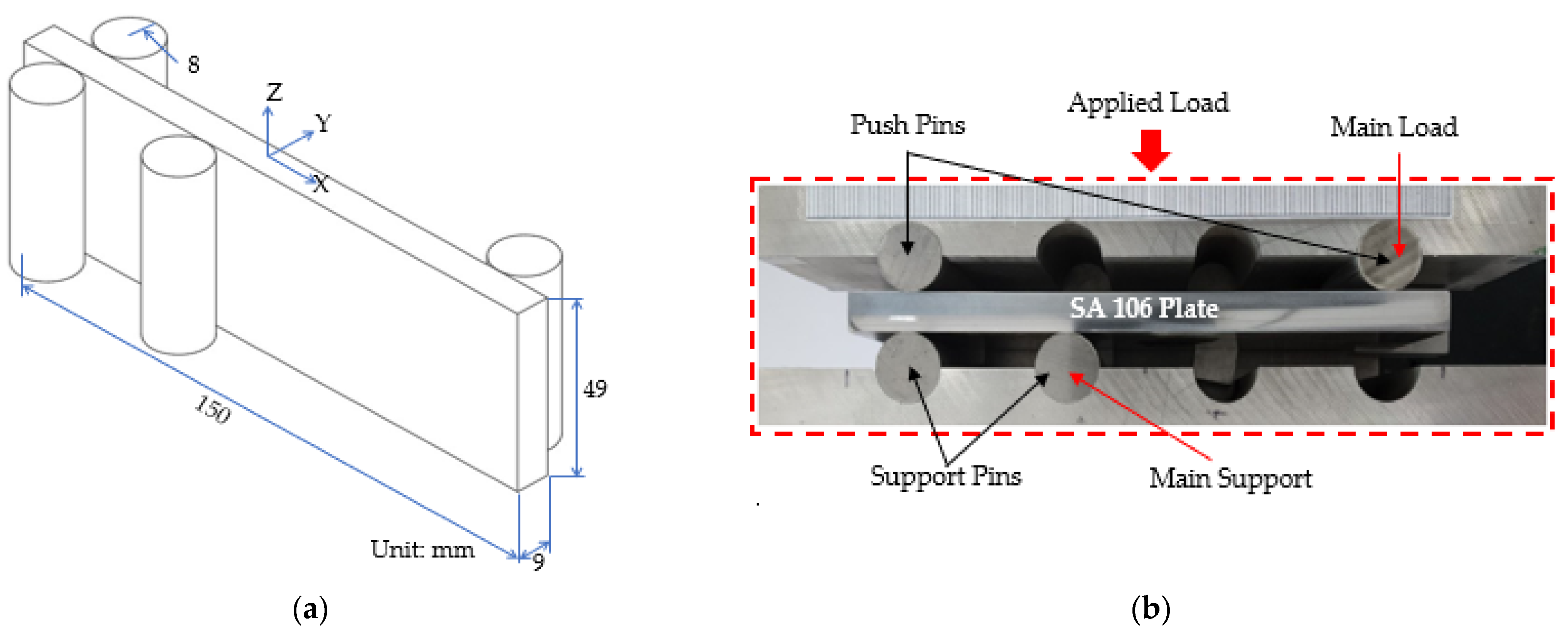
2. Materials and Methods

The equipment used in the experiment consists of a signal processing circuit, a carbon steel specimen, a power supply, a three-directional TMR sensor, and a loading system. The inspection setup block diagram is streamlined in Figure 1a. The I/O controller of the NI-USB device is employed to monitor the power supplied to the sensor, and the signal processing circuitry. The output signal from the TMR sensor is processed by high-pass filters, amplifiers, and root mean square (RMS) measurement circuits into a continuous signal that is digitized by the NI-USB A/D converter, and ultimately appears as software on a laptop. The XY stage is translated by a motor which is controlled by LabVIEW software via the USB port.

The magnetic flux density ($\overrightarrow{B}$) in space resulting from an external magnetic field ($\overrightarrow{H}$) and the magnetization ($\overrightarrow{M}$) in the ferromagnetic material is outlined below:

$$\overrightarrow{B}={\mu }_0\overrightarrow{H}+{\mu }_0\overrightarrow{M}$$

(1)

where the magnetization vector can be defined as the total sum of the magnetic dipole moments expressed as [39]:

$$\overrightarrow{M}=\underset{\mathsf{\Delta }v\to 0}{lim}\frac{{{\displaystyle \sum }}_{k=1}^{n\mathsf{\Delta }v}{m}_k}{\mathsf{\Delta }v}$$

(2)

with $m_k$ being the magnetic dipole moment. Even $\overrightarrow{H}=0$, but $\overrightarrow{M}\ne 0$ with a stress strain condition, meaning that even without $\overrightarrow{H}$, $\overrightarrow{B}$ is not equal to zero [40].

To measure the $\overrightarrow{B}$ in MMM, the flux gate is used in most cases, and the following expression is used:

$$V_{emf}=-\frac{d\varnothing }{dt}=\underset{S}{{\displaystyle \int }}\left(-\frac{\partial \overrightarrow{B}}{dt}\right) \overrightarrow{ds}$$

(3)

where $\frac{\partial \overrightarrow{B}}{dt}$ is the frequency of excitation, and s is the area of the coil.

In the rod type flux gate, which is used for the MMM usually, the lift-off is very small, the primary coil to detect ${{\displaystyle \int }}_s^{.}\left(-\frac{\partial \overrightarrow{B}}{dt}\right) \overrightarrow{ds}$ generates the magnetic field, as the lift-off is too close to the inspected material, so magnetic field occur; the effect is small, but it exists.

In the case of the TMR sensor used in this paper, the output voltage is given by the Formula (4) [41]:

$$V_{TMR}=2\frac{k{V}_s}{R}∆B$$

(4)

where $V_s$ is the applied voltage, R is the resistance of the TMR sensor, and $k$ is a constant parameter of the sensor.

The change in the TMR output is the consequence of stress. Changes in magnetization are caused by the applied mechanical stress, and can be inferred. Moreover, the TMR offers a very small measuring point.

The experimental equipment is shown in Figure 1b, whereas the properties are given in

Table 1. Properties of the SA 106 specimen.

Parameter	Value
Young’s modulus	210 GPa
Poisson ratio	0.3
Relative permeability	260

, and the schematic of the four-point loading test, including the shape and the dimensions of the SA 106 plate, is illustrated in Figure 2.

To figure out and estimate the 3D stress distribution on the target carbon steel plate, the latter was subjected to two load levels equivalent to the displacement (0 and 0.1 mm), undertaken inside a laboratory at ambient temperature using a four-point stainless steel loading test so as not to influence the signal recovered by the TMR sensor. The plate was pushed in one side by two pins and two support pins: two pins in the same side and the other two in the other side, as shown in Figure 2b. The stress induces a primary magnetic field, which flows through the carbon steel plate, and a three-dimensional TMR sensor performed a c-scan on the upper surface of the plate to measure the three components of the magnetic flux distribution over the specimen while the load was still in place. The lift-off was held at 0.3 mm, and just prior to applying the load, the contact positions between the specimen and the pins were checked. After the first measurement, the equivalent displacement was gingerly applied, and the load was raised to the next level without unloading.

3. Results, Analysis, and Discussion

To understand and meaningfully probe the stress distribution, and yield relevant information concerning the stress behavior of the SA 106 plate subjected to compressive stress, illustrated in the second section, an appropriate investigational test procedure and simulation are requisite. To this end, the stress distributions derived from the finite element modeling are complementary to the experimental measurement of the magnetic flux density measurement. The modeling of the stress distribution on the SA 106 specimen has brought an invaluable contribution to this study. The coherence of the FEM analysis with the experimental measurements has been outlined, thereby allowing the results of the FEM stress modeling to be a trustworthy representation of the real state. The general intention of the experimental and simulation work was to find a relationship that would allow an evaluation of the state of the tested plate with the stresses to which it was subjected.

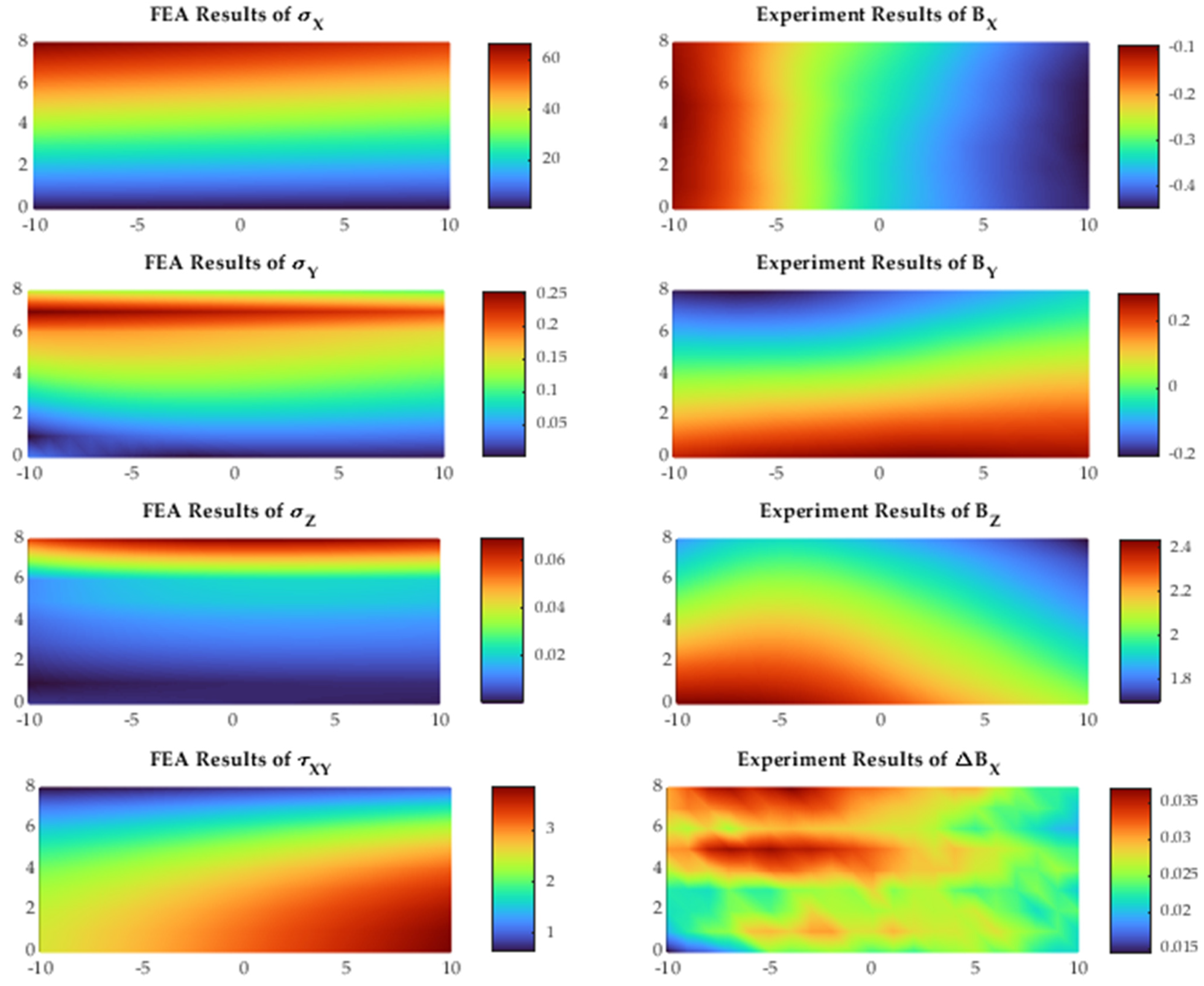
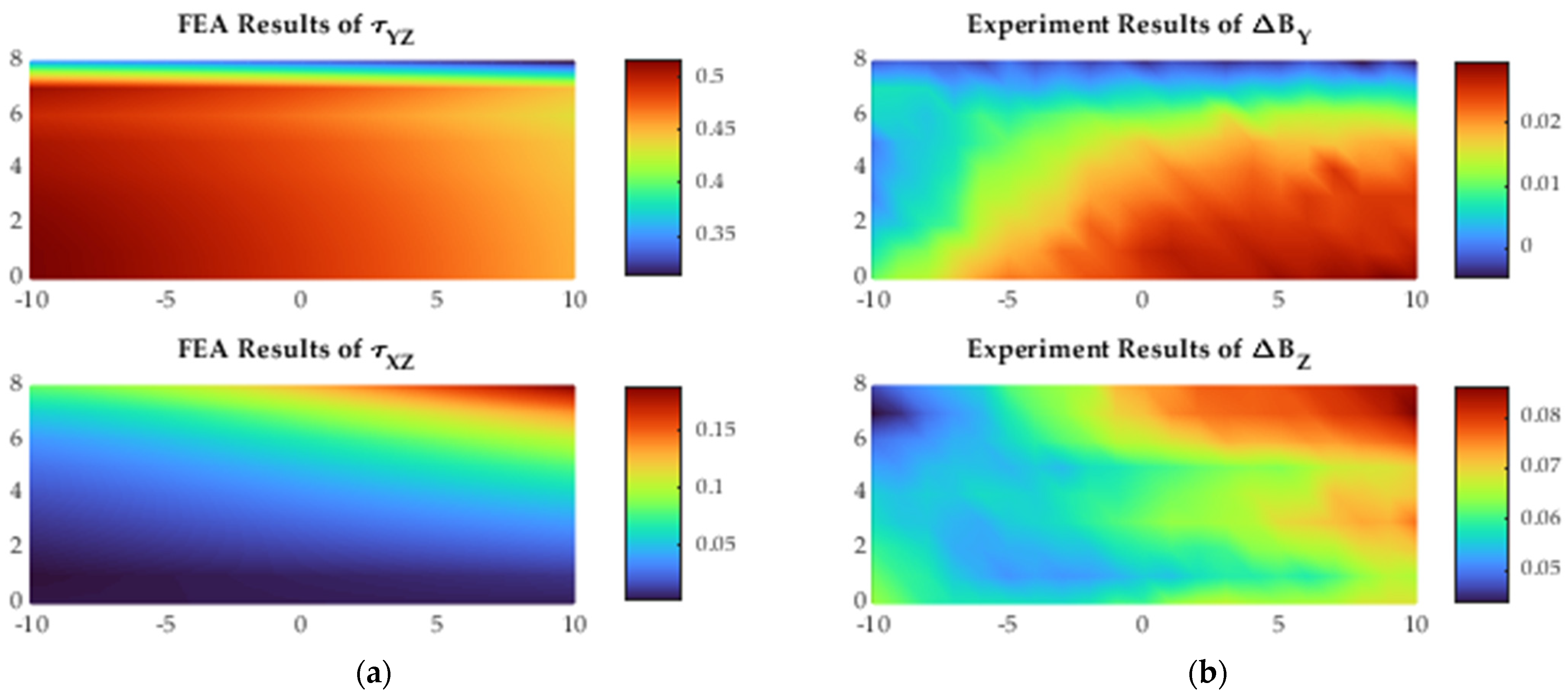
3.1. Experiments Results

In this part, the measurement data obtained with the sensor are presented, and they were taken following the experimental procedure outlined in the Materials and Methods section. They provided a dataset for each applied load, where signals were acquired for the three X, Y, and Z directions.

The collected experimental data are shown in Figure 3. The analysis of the magnetic flux density represented by Figure 3a is somewhat tricky and can lead to confusion if these data are analyzed in terms of $B_X$, $B_Y$, and $B_Z$, and it is complex to evaluate the loading condition of the plate under study. In general, it is difficult to absolutize the magnetic field according to the in-situ state, on account of the geomagnetic field, the background, and the residues, so it is necessary to compare with the reference. To overcome this limitation, a differential magnetic flux density is used, and is computed by:

$$∆{\mathrm{B}}_{\alpha }={\mathrm{B}}_{\alpha ,def}-{\mathrm{B}}_{\alpha ,0.00}$$

(5)

where α means the components X, Y, and Z; ${\mathrm{B}}_{\alpha ,def}$ is the magnetic flux density at each deformation; and ${\mathrm{B}}_{\alpha ,0.00}$ is the magnetic flux density without deformation.

The back data (magnetic flux density without deformation) were subtracted from the magnetic flux to delete the bias, as presented in Figure 3b, and the resulting data were plotted in terms of $\mathsf{\Delta }{B}_X$, $\mathsf{\Delta }{B}_Y$, and $\mathsf{\Delta }{B}_Z$, which is particularly beneficial in making the changes visible; furthermore, the achieved data reveal the differences that are clearly visible, and show changes in the parameter’s values over the surface of the plate, even in terms of amplitude for the applied load.

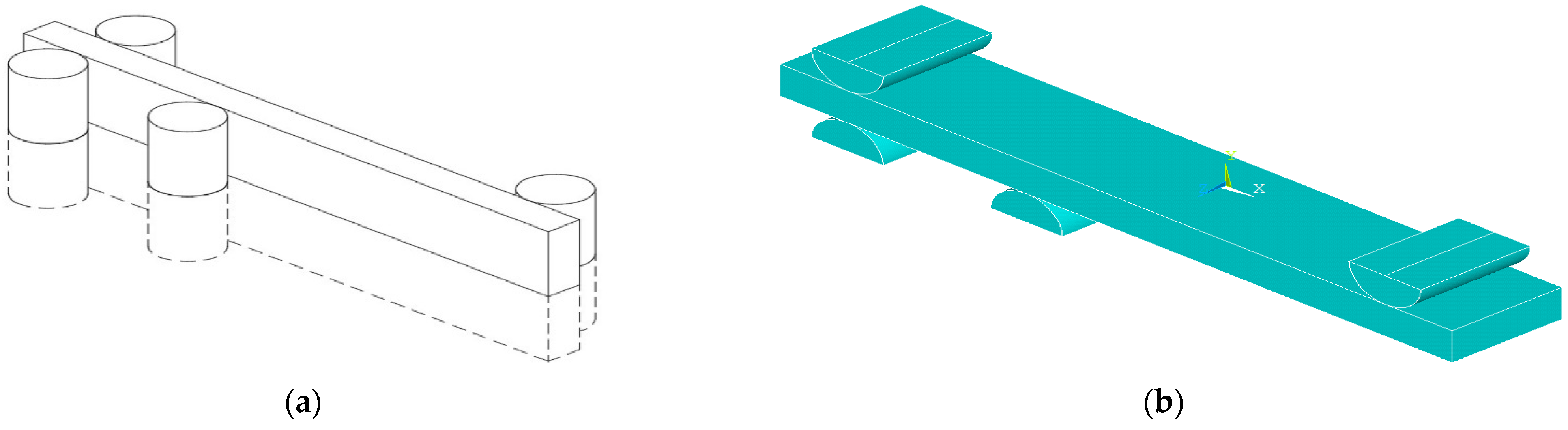
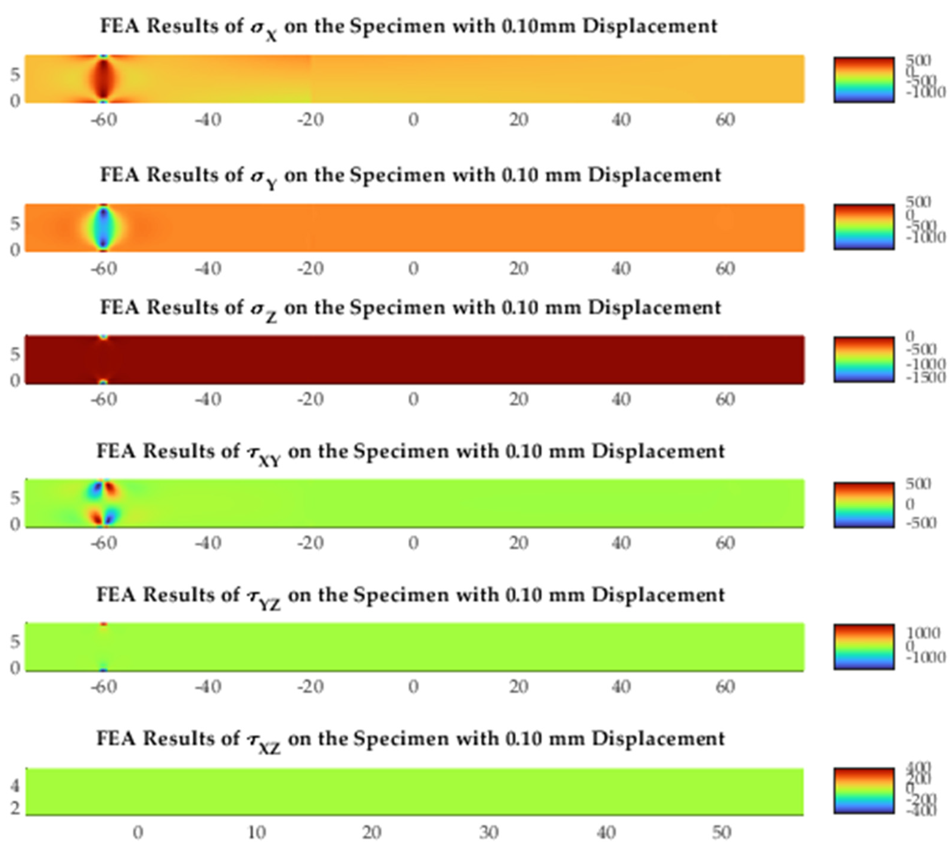
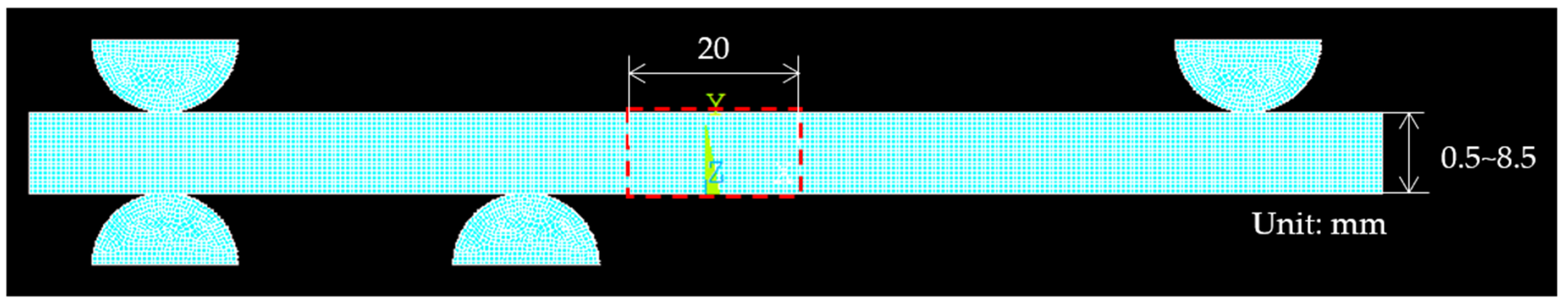
3.2. Finite Element Analysis

Ansys FEM simulation software was deployed to perform and analyze the stress distribution and concentration in the X, Y, and Z directions of the SA 106 specimen under different compressive loads. The free boundary condition was applied on one side of the model, and the pushing tensile force was applied on the other side. The three-dimensional model automatic meshing methods adopted tetrahedral and hexahedral elements. The size of mesh elements was chosen to be 0.5 mm in order to create an efficient mesh with regular sizing through the volume and the faces. As three-dimensional FEM models are time-consuming, to save mesh and resolution time, only a half-symmetry of the plate was simulated, and it is shown in Figure 4.

The distributions and intensities of stress and shear stress on the SA 106 plate applied by the four-point loading system were simulated using the Ansys software. The FEM was conducted for 0.1 mm displacement along the three directions, as shown in Figure 5. It can be observed that there is a concentration around the −60 mm position on the bottom and upper sides, which corresponds to the position of the two left pins, where the range of ${\mathsf{\sigma }}_X$ and ${\mathsf{\sigma }}_Y$ is higher than ${\mathsf{\sigma }}_Z$.

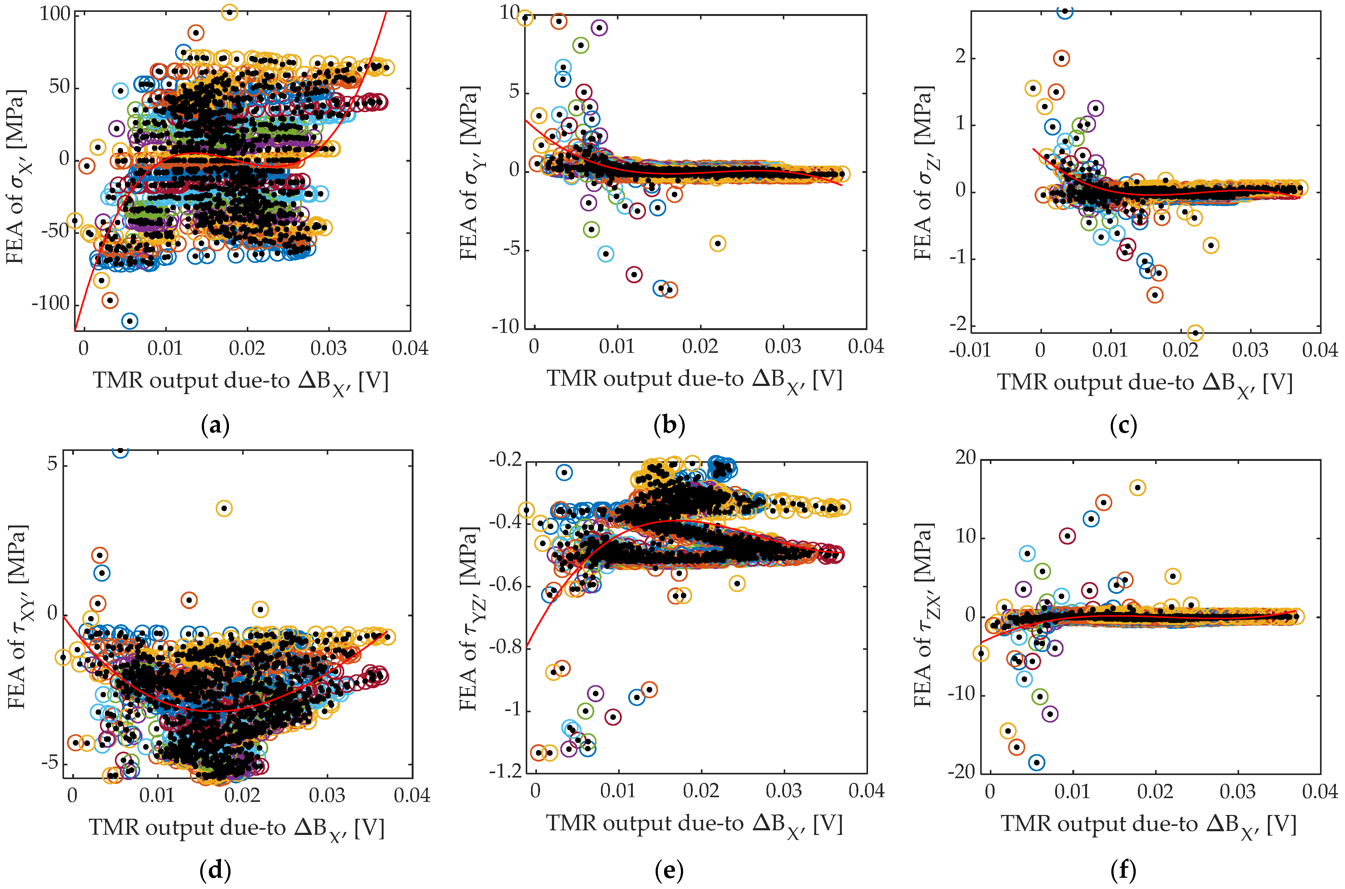
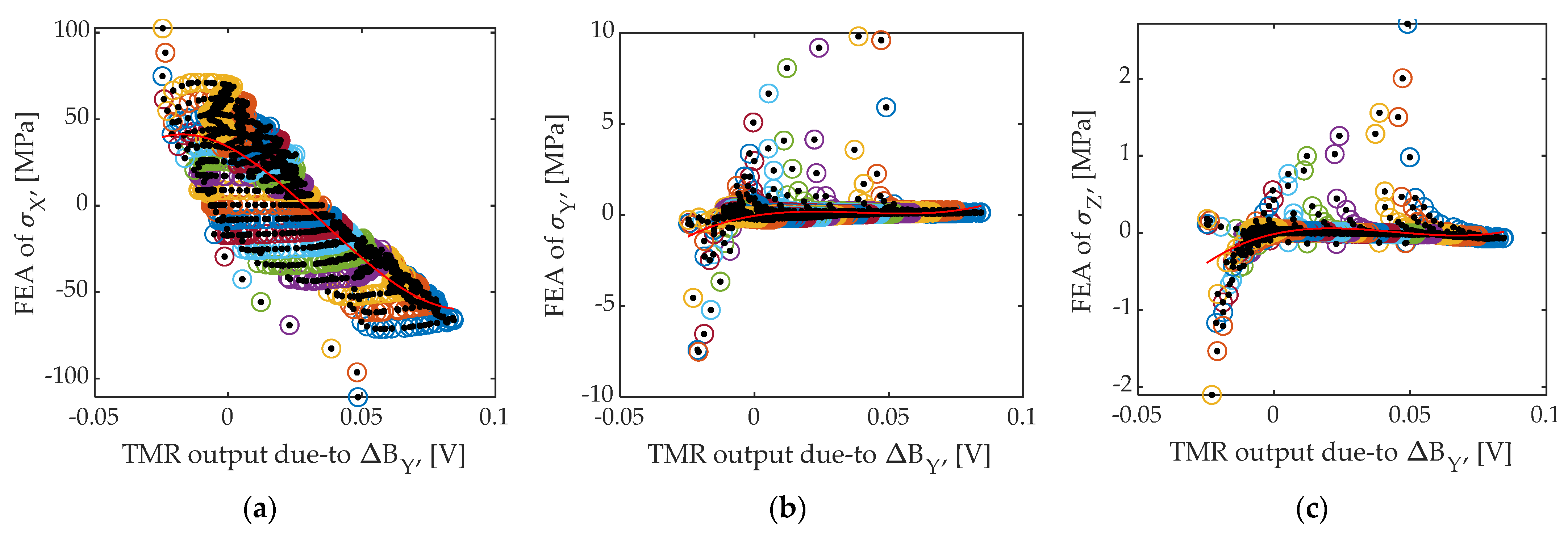
3.3. Analysis Area and Comparison

The focus of this part was to compare the distribution of the stress simulated by the finite element analysis and the variations of the measured magnetic flux density, in order to determine the differential magnetic flux density and the stress distributions on the specimen when applying the load. In the comparison between the two datasets, the same target area was selected. The center of the selected area corresponds to the center of the plate for the simulation and experiment, and 10 mm before and after the center line were selected to conduct the study by matching the two areas, as shown by the red dashed line, and to avoid the pinning effect and edge effect, as shown in Figure 6.

Figure 7 illustrates the variation of stress and shear stress obtained by the software, as well as the magnetic flux density and differential magnetic flux density obtained by the experiment. It can be observed that for the FEM results, the principal stress distribution follows the x direction; in other words, the range of ${\mathsf{\sigma }}_X$ is the more significant stress than of ${\mathsf{\sigma }}_Y$ and ${\mathsf{\sigma }}_Z$, where ${\mathsf{\sigma }}_Z$ is the least significant stress. An almost identical feature is observed for the three stresses. The shear stresses, ${\tau }_{XY}$, ${\tau }_{YZ}$, and ${\tau }_{XZ}$, show a variant distribution: upward and leftward variation, upward and rightward variation, and downward and leftward variation, respectively. They appear to be small, but larger than the least significant stress, especially ${\tau }_{XY}$.

$B_X$ varies from left to right, and $B_Y$ varies from bottom to top; $B_Z$ is a mixture of the two trends of $B_X$ and $B_Y$ (upward and rightward variation). Furthermore, the obtained results show that the behavior of the differential magnetic flux density ($\mathsf{\Delta }{B}_X$, $\mathsf{\Delta }{B}_Y$, and $\mathsf{\Delta }{B}_Z$) is not uniform, and coincides with the simulated stress and shear stress.

It turns out that the simulated data have, more or less, a resemblance to the measured data; although, there are some differences. However, a graded variation tendency can be seen, and a good correlation is also observed, mainly with the differential magnetic flux density. This implies that there is a good match between the results. This first step of comparison can be used as a criterion to judge the efficiency of the simulation. These results will be used to evaluate the stresses depending on the differential flux density.

In several cases, the simulated and measured data have the same trend, but it is rather difficult to make an analysis by focusing only on one of them or their behavior. In the following, an attempt is made to find relationships between the two data (Figure 8, Figure 9 and Figure 10). Since the $\mathsf{\Delta }{B}_X$ data are small, on the order of 0.04 and 0.15 for both $\mathsf{\Delta }{B}_Y$ and $\mathsf{\Delta }{B}_Z$, the Tylor series can be used to approximate these data in polynomial form. On the other hand, the Taylor series computation merely involves the function’s acquaintance with the proximity of a point. Therefore, working with the Taylor series results in a considerably small error in the proximity of the point where it is calculated.

The Taylor series of a function is an infinite sum of its derivatives at a single point, as given below [42,43]:

$$T\left\{\left(f\left(x\right)\right)\right\}={\displaystyle \sum }_{n=0}^{\infty }\frac{f^{\left(n\right)}\left(a\right)}{n!}{\left(x-a\right)}^n$$

(6)

where $T\left\{\left(f\left(x\right)\right)\right\}$ denotes the Taylor series of a real valuated function, $f\left(x\right)$; the right-hand side is called the $n$th Taylor polynomial, and $n$ takes on non-negative integer values; $n!$ is the factorial of $n$; and $f^{\left(n\right)}\left(a\right)$ is the $n$th derivative of the function, $f\left(x\right)$, evaluated at the point $x=a$.

Note that the partial sums of the series are broadly used to approximate the function. The accuracy of the approximation increases with the number of terms included. However, underneath, the third-order polynomial type is used, which is accurate and sufficient to handle the presented data. By taking advantage of this type of polynomial, the stresses and shear stresses (${\mathsf{\sigma }}_{\alpha }$ and ${\tau }_{\beta }$) are approximated by the differential magnetic flux density, $\mathsf{\Delta }{B}_{\alpha }$, in the form of a third-order polynomial functional relation as [44]:

$${\mathsf{\sigma }}_{\alpha }.{\tau }_{\beta }=p_0+p_1 \mathsf{\Delta }{B}_{\alpha }+p_2 \mathsf{\Delta }{B}_{\alpha }{}^2+p_3 \mathsf{\Delta }{B}_{\alpha }{}^3$$

(7)

where ${\mathsf{\sigma }}_{\alpha }.{\tau }_{\beta }$ means both ${\mathsf{\sigma }}_{\alpha }$ or ${\tau }_{\beta }$ are used, but independently; $p_0$,$p_1$,$p_2$, and $p_3$ denote the transformations coefficients; α: (X, Y, Z) and β: (XY, YZ, ZX).

The approximated data by the Equation (7) study the relationship between the stress and shear stress versus the differential magnetic flux density. The error between the approximated data and the experimented data is expressed by the following formula:

$$E_{\alpha }=\frac{\sum {\left({\left({\mathsf{\sigma }}_{\alpha }.{\tau }_{\beta }\right)}_{approximated}-{\left({\mathsf{\sigma }}_{\alpha }.{\tau }_{\beta }\right)}_{experimented}\right)}^2}{\sum {\left({\mathsf{\sigma }}_{\alpha }.{\tau }_{\beta }\right)}_{experimented}{}^2}$$

(8)

The purpose of calculating the error is to determine whether the marriage Equation (7) for estimating the data is accurate; in other words, whether the behavior of the data is accurately reflected by the equation applied. As a guideline, Figure 8a–f, Figure 9a–f, and Figure 10a–f correspond to Cases 1–6, 7–12, and 13–18, respectively, as portrayed in

Table 2. Values of the transformation coefficients, error, and features for each case.

Case	Transformation Coefficient Values, Error, and Features
	1st Coefficient $\left({\mathit{p}}_0\right)$	2nd Coefficient $\left({\mathit{p}}_1\right)$	3rd Coefficient $\left({\mathit{p}}_2\right)$	$4\mathbf{th} \mathbf{Coefficient} \left({\mathit{p}}_3\right)$	$\mathbf{Error} \left(\sqrt{{\mathit{E}}_{\mathit{\alpha }}}\right)$	Constancy (C)	$\mathbf{Linearity} \left(\mathit{L}\right)$
1	−94.5	$1.841\times {10}^4$	$-1.082\times {10}^6$	$1.968\times {10}^7$	0.0316	$4.5476\times {10}^{-6}$	$8.8671\times {10}^{-4}$
2	2.78	−445.5	$2.203\times {10}^4$	$-3.416\times {10}^5$	0.0906	$7.6358\times {10}^{-6}$	0.0012
3	0.543	−89.72	4366	$-6.493\times {10}^4$	0.0975	$7.8258\times {10}^{-6}$	0.0013
4	−0.4634	−362.1	$1.35\times$104	$-1.018\times {10}^5$	0.0300	$4.0065\times {10}^{-6}$	0.0031
5	−0.7341	47.89	−2050	$2.52\times {10}^4$	0.0283	$2.6892\times {10}^{-5}$	0.0018
6	−2.642	461.2	$-2.377\times {10}^4$	$3.742\times {10}^5$	0.1345	$6.6310\times {10}^{-6}$	0.0012
7	33.92	−792.9	$-1.853\times {10}^4$	$1.752\times {10}^5$	0.0316	$1.7437\times {10}^{-4}$	0.0041
8	−0.04409	23.83	−743.2	6368	0.0900	$6.1794\times {10}^{-6}$	0.0034
9	−0.01645	7.931	−248.5	1880	0.0980	$7.6998\times {10}^{-6}$	0.0037
10	−2.355	−55.7	22.79	$1.312\times {10}^4$	0.0300	$1.7843\times {10}^{-4}$	0.0042
11	−0.4443	3.218	−104.3	1048	0.0300	$3.8450\times {10}^{-4}$	0.0028
12	0.2511	−66.29	2156	$-1.86\times {10}^5$	0.1353	$1.3341\times {10}^{-6}$	$3.5231\times {10}^{-4}$
13	−46.01	763.3	4817	$-3.596\times {10}^4$	0.0316	0.0011	0.0187
14	0	−2.472	−143.8	1512	0.0906	0	0.0015
15	0.04189	−0.2911	−52.87	678.8	0.1015	$5.7230\times {10}^{-5}$	$3.9783\times {10}^{-4}$
16	−1.643	−31.71	−196	4541	0.0949	$3.4454\times {10}^{-4}$	0.0067
17	−0.384	−1.047	−40.25	672.9	0.0316	$5.3767\times {10}^{-4}$	0.0015
18	−0.4819	2.362	319.4	−3229	0.1342	$1.3572\times {10}^{-4}$	$6.6556\times {10}^{-4}$

.

Figure 8, Figure 9 and Figure 10 reveal two distribution patterns: a gradient distribution between each data, and a gradient distribution of the whole. ${\mathsf{\sigma }}_X$ versus the differential magnetic flux density describes a strong relationship, as ${\mathsf{\sigma }}_X$ represents the principal stress with more significant magnitude than ${\mathsf{\sigma }}_Y$ and ${\mathsf{\sigma }}_Z$. In Figure 8a, a perfect third polynomial trend is observed, whereas ${\mathsf{\sigma }}_X$ exhibits an approximately linear change, with indirect and direct slopes in Figure 9a and Figure 10a, respectively. Both ${\mathsf{\sigma }}_Y$ and ${\mathsf{\sigma }}_Z$ plot an almost horizontal trend in Figure 8b,c, although ${\mathsf{\sigma }}_Y$ is higher than ${\mathsf{\sigma }}_Z$, and the same trend is also seen in Figure 9b,c, without significant variation, and an approximately constant trend in Figure 10b,c. In all cases, ${\mathsf{\sigma }}_X$ yields a better response. ${\tau }_{XY}$ shows a curve variation with a downward peak, whereas ${\tau }_{YZ}$ depicts a perfect polynomial trend with a small amplitude variation. ${\tau }_{ZX}$ exhibits an approximately horizontal trend, with small amplitude variation in Figure 8d and Figure 9d, and keeps a nearly constant variation in Figure 10d.

There is a good correlation between the quantities represented. This ascertainment leads to the assumption that these quantities are complementary to each other. It is obvious that these findings may differ; however, the fundamental tendency of the variations is basically the same. Incidentally, similar trends appear, in certain cases, to be well correlated; therefore, it is reasonable to conclude that the relationship can be well characterized for both the stresses and shear stresses.

Moreover, by taking a closer look at the coefficients, $p_0$, $p_1$, $p_2$, and $p_3$, shown in Table 2, some features can be established; among them, the constancy ($C$) and linearity described in Equations (9) and (10), and portrayed in Figure 11:

$$C=\frac{\left|p_0\right| }{ \left|p_1\right|+\left|p_2\right|+\left|p_3\right|}$$

(9)

$$L=\frac{\left|p_1\right| }{ \left|p_0\right|+\left|p_2\right|+\left|p_3\right|}$$

(10)

Detailed information regarding the error and the characteristics is provided in Figure 11. These data serve as a guideline for classifying cases that possess the appropriate relationship. In Figure 8a–f, which represent cases 1 to 6, the $\mathsf{\Delta }{B}_X$ range is small because the sensitivity of the sensor is high; for a proper assessment, these are not included in the analysis of Table 2 and Figure 11.

As an indication of the datum quality by the given Equations (8)–(10), a data plot of these data from 18 cases is presented in Figure 11. The error quality was obtained by dividing the sum of the squared errors by the sum of the squared constraints, as indicated by Equation (8). The error range is 0.0316 to 0.1353 (3.16% to 13.53%); however, not all errors are acceptable; cases 7 and 10 are optimal. There is, indeed, a good constancy in cases 8, 9, and 12. Furthermore, a good linearity is also observed in cases 7, 13, and 16.

As a result of the applied load, the magnetic data measurable by the TMR sensor change in response to the domain motion. The variations of the magnetic signals in the ferromagnetic plate under the effect of the applied load were used as a means for the MMM to be performed, i.e., the changes in the magnetic properties of the ferromagnetic specimen under the effect of the applied load. Thus, these affect the direction and structure of the domains, and produce a magnetic moment on the specimen. According to existing knowledge in the literature, in the ferromagnetic system, the domains can be aligned or randomly aligned according to the presence or absence or of an external magnetic field, respectively; magnetic alterations in ferromagnetic materials can be assigned to the change in the structure of the magnetic domains.

The central intent of this investigation was to seek the relationship between the measured triaxial magnetic flux density and the simulated stress and shear stress by the Ansys software, allowing one to assess the state of the tested SA 106 plate.

It was found that ${\mathsf{\sigma }}_Z$ is smaller than ${\mathsf{\sigma }}_X$ and ${\mathsf{\sigma }}_Y$, and maintains a nearly constant trend and value, as there is little or no residual magnetization on the plate along the Z directions. On the other hand, ${\mathsf{\sigma }}_X$, ${\mathsf{\sigma }}_Y$, and ${\tau }_{XY}$ are affected, and show a visible change in attention in such a loading configuration.

It was tough to explain the relationship between each stress and shear stress as a function of the magnetic flux density presented in Figure 8, Figure 9 and Figure 10, so it was important to find an alternative that guaranteed clear relationships; hence, the use of a third-order polynomial equation type to obtain clear relationships that help understand the effect of the stress, and to achieve the goal set in the beginning.

By the time the material is first subjected to a modest load, it adopts an elastic behavior by stretching its atomic boundaries, where stiffness is considered as the ability of the material to resist deformation when acted upon by external stress. Elastic behavior essentially implies that regardless of the movement of the material when stressed, it returns to its initial stance when the load is released. The ratio between the stress and the elastic deformation is known as Young’s modulus. However, if this elastic deformation is exceeded and the yield strength is reached, the material undergoes permanent deformation. To safeguard security, it is very important that the working range of our materials used in various constructions and transportations in everyday life remain in the elastic regime, so the material does not undergo any permanent deformation.

An important inference is the need to search for the relationship using the shear stress, and not just with each direction of stress to obtain the latter. As pointed out above, the last figure shows an obvious correlation and identification of the relationships obtained. These relationships are pivotal in identifying the state of the stressed plate for the purposes of establishing a preventive approach method for possible use in several applications in the upcoming timeframe.

4. Conclusions

In this paper, a nondestructive testing method, based on the metal magnetic memory effect of a carbon steel plate (SA 106) subjected to compressive stresses, was carried out by finite element simulation and experimentation. Both the software-simulated stress distribution and the triaxial flux density measurement were mined to gauge their usability and applicability in such an engineered application. On the basis of the findings, it is advocated to utilize not only stress distribution to gauge the material status, but the shear stress as well. The following items from the used loading configuration can be emphasized:

• The stresses along both X and Y directions, and the shear stress on the XY plan are affected.
• The magnetic flux density along the Y and Z direction is affected too.
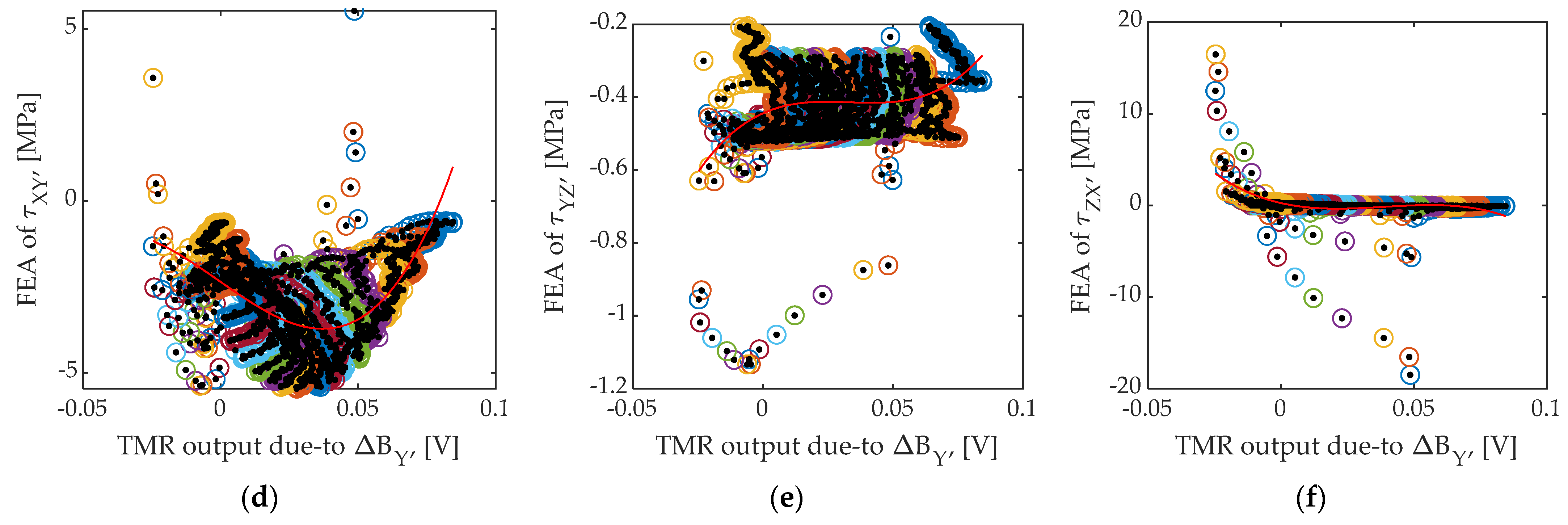
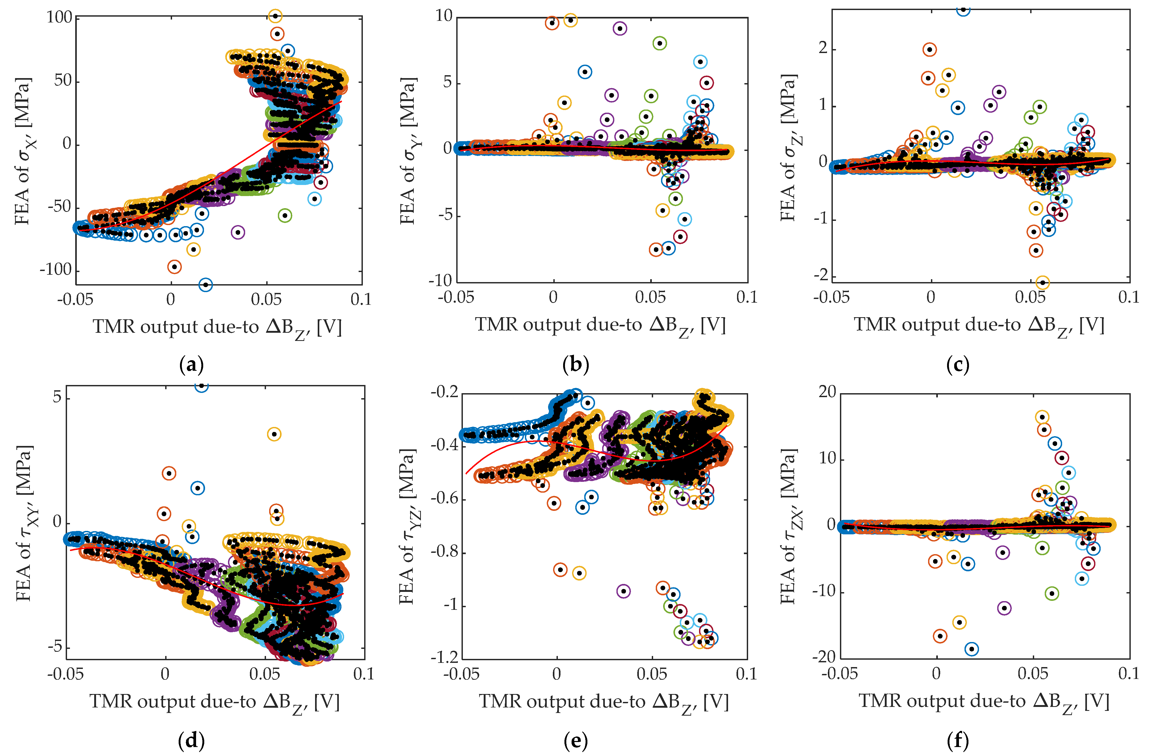
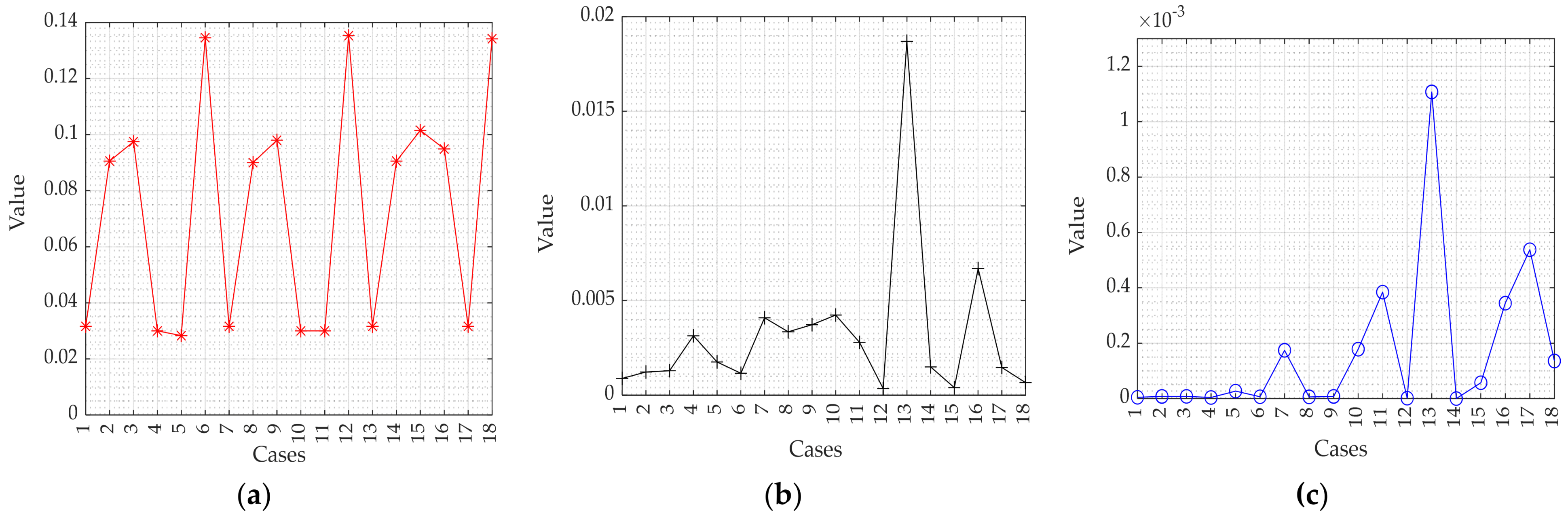
• In addition, a qualitative relationship in the form of a third-order polynomial equation has been established, which is based on correlations between the stress distributions and shear stress as a function of the recovered triaxial magnetic field. The error and features resulting from the application to ascertain relationships seems to be entirely reasonable in some cases (not in all cases); indeed, these points highlight a good relationship:
• The stress along the X direction, representing the main stress;
• The vertical differential flux density, the appropriate parameter for stress characterization;
• Although MMM can be used to inspect the stress, it is cumbersome to qualitatively assess the stress because of the error.

Furthermore, the data presented can be used for the prediction and verification of specimen performance and structural health. Another important consideration is the use of a sensitive sensor for such an application, due to the low flux produced by the compressive stress.

References

1. Sumi, Y. Stress Concentration Problems. In Mathematical and Computational Analyses of Cracking Formation; Mathematics for Industry; Springer: Tokyo, Japan, 2014; Volume 2, pp. 17–30. [Google Scholar] [CrossRef]
2. Le, M.; Kim, J.; Yang, D.; Lee, H.; Lee, J. Electromagnetic testing of a welding area using a magnetic sensor array. Int. J. Appl. Electromagn. 2017, 55, 119–124. [Google Scholar] [CrossRef]
3. Wang, G.; Yan, P.; Wei, L.; Deng, Z. The Magnetic Memory Effect of Ferromagnetic Materials in the Process of Stress-Magnetism Coupling. Adv. Mater. Sci. Eng. 2017, 2017, 1284560. [Google Scholar] [CrossRef] [Green Version]
4. Zhou, W.; Fan, J.; Ni, J.; Liu, S. Variation of Magnetic Memory Signals in Fatigue Crack Initiation and Propagation Behavior. Metals 2019, 9, 89. [Google Scholar] [CrossRef] [Green Version]
5. Villegas-Saucillo, J.J.; Díaz-Carmona, J.J.; Cerón-Álvarez, C.A.; Juárez-Aguirre, R.; Domínguez-Nicolás, S.M.; López-Huerta, F.; Herrera-May, A.L. Measurement System of Metal Magnetic Memory Method Signals around Rectangular Defects of a Ferromagnetic Pipe. Appl. Sci. 2019, 9, 2695. [Google Scholar] [CrossRef] [Green Version]
6. Herter, S.; Youssef, S.; Becker, M.M.; Fischer, S.C. Machine Learning Based Preprocessing to Ensure Validity of Cross-Correlated Ultrasound Signals for Time-of-Flight Measurements. J. Nondestruct. Eval. 2021, 40, 20. [Google Scholar] [CrossRef]
7. Berkache, A.; Lee, J.; Choe, E. Evaluation of Cracks on the Welding of Austenitic Stainless Steel Using Experimental and Numerical Techniques. Appl. Sci. 2021, 11, 2182. [Google Scholar] [CrossRef]
8. Lee, J.; Berkache, A.; Wang, D.; Hwang, Y.-H. Three-Dimensional Imaging of Metallic Grain by Stacking the Microscopic Images. Appl. Sci. 2021, 11, 7787. [Google Scholar] [CrossRef]
9. Berkache, A.; Lee, J.; Wang, D.; Park, D.-G. Development of an Eddy Current Test Configuration for Welded Carbon Steel Pipes under the Change in Physical Properties. Appl. Sci. 2022, 12, 93. [Google Scholar] [CrossRef]
10. Diguet, G.; Miyauchi, H.; Takeda, S.; Uchimoto, T.; Mary, N.; Takagi, T.; Abe, H. EMAR monitoring system applied to the thickness reduction of carbon steel in a corrosive environment. Corrosion 2022, 73, 658–668. [Google Scholar] [CrossRef]
11. International Atomic Energy Agency. Liquid Penetrant and Magnetic Particle Testing at Level 2; International Atomic Energy Agency (IAEA): Vienna, Austria, 2000. [Google Scholar]
12. Berkache, A.; Oudni, Z.; Mehaddene, H.; Mohellebi, H.; Lee, J. Inspection and characterization of random physical property efects by stochastic finite element method. Prz. Elektrotech. 2019, 95, 96–101. [Google Scholar] [CrossRef]
13. Huang, L.; Liao, C.; Song, X.; Chen, T.; Zhang, X.; Deng, Z. Research on Detection Mechanism of Weld Defects of Carbon Steel Plate Based on Orthogonal Axial Eddy Current Probe. Sensors 2020, 20, 5515. [Google Scholar] [CrossRef]
14. Krkoška, L. Investigation of Barkhausen Noise Emission in Steel Wires Subjected to Different Surface Treatments. Coatings 2020, 10, 912. [Google Scholar] [CrossRef]
15. O’Sullivan, D.; Cotterell, M.; Cassidy, S.; Tanner, D.A.; Mészárosc, I. Magneto-acoustic emission for the characterisation of ferritic stainless steel microstructural state. J. Magn. Magn. Mater. 2004, 271, 381–389. [Google Scholar] [CrossRef] [Green Version]
16. Tang, J.; Wang, R.; Qiu, G.; Hu, Y.; Kang, Y. Mechanism of Magnetic Flux Leakage Detection Method Based on the Slotted Ferromagnetic Lift-Off Layer. Sensors 2022, 22, 3587. [Google Scholar] [CrossRef]
17. Leng, J.; Xu, M.; Zhou, G.; Wu, Z. Effect of initial remanent states on the variation of magnetic memory signals. NDT E Int. 2012, 52, 23–27. [Google Scholar] [CrossRef]
18. Pengpeng, S.; Ke, J.; Xiaojing, Z. A magnetomechanical model for the magnetic memory method. Int. J. Mech. Sci. 2017, 124–125, 229–241. [Google Scholar] [CrossRef]
19. Bao, S.; Jin, P.; Zhao, Z.; Fu, M. A Review of the Metal Magnetic Memory Method. J. Nondestruct. Eval. 2020, 39, 11. [Google Scholar] [CrossRef]
20. Zhang, Z. Wavelet Energy Entropy Based Multi-Sensor Data Fusion for Residual Stress Measurement Using Innovative IntenseMagnetic Memory Method. In Proceedings of the 2009 9th International Conference on Electronic Measurement Instruments, Beijing, China, 16–19 August 2009; pp. 1044–1047. [Google Scholar] [CrossRef]
21. Chady, T.; Łukaszuk, R. Examining Ferromagnetic Materials Subjected to a Static Stress Load Using the Magnetic Method. Materials 2021, 14, 3455. [Google Scholar] [CrossRef]
22. Dubov, A.A. A study of metal properties using the method of magnetic memory. Metal. Sci. Heat Treat. 1997, 39, 401–405. [Google Scholar] [CrossRef]
23. Dubov, A.; Dubov, A. Application of the metal magnetic memory method for detection of defects at the initial stage of their development for prevention of failures of power engineering welded steel structures and steam turbine parts. Weld. World 2014, 58, 225–236. [Google Scholar] [CrossRef]
24. Shi, P.; Jin, K.; Zhang, P.; Xie, S.; Chen, Z.; Zheng, X. Quantitative Inversion of Stress and Crack in Ferromagnetic Materials Based on Metal Magnetic Memory Method. IEEE Trans. Magn. 2018, 54, 1–11. [Google Scholar] [CrossRef]
25. Ren, S.; Ren, X.; Duan, Z.; Fu, Y. Studies on influences of initial magnetization state on metal magnetic memory signal. NDT E Int. 2019, 103, 77–83. [Google Scholar] [CrossRef]
26. Chady, T.; Łukaszuk, R.D.; Gorący, K.; Żwir, M.J. Magnetic Recording Method (MRM) for Nondestructive Evaluation of Ferromagnetic Materials. Materials 2022, 15, 630. [Google Scholar] [CrossRef]
27. Roskosz, M. Metal magnetic memory testing of welded joints of ferritic and austenitic steels. NDT E Int. 2011, 44, 305–310. [Google Scholar] [CrossRef]
28. Dubov, A.; Kolokolnikov, S. Assessment of the material state of oil and gas pipeline based on the metal magnetic memory method. Weld. World 2012, 56, 11–19. [Google Scholar] [CrossRef]
29. Witoś, M. The MMM expert system: From a reference signal to the method validation. Fatigue Aircr. Struct. 2012, 1, 123–140. [Google Scholar] [CrossRef]
30. Huang, H.; Jiang, S.; Liu, R.; Liu, Z. Investigation of magnetic memory signals induced by dynamic bending load in fatigue crack propagation process of structural steel. J. Nondestruct. Eval. 2014, 33, 407–412. [Google Scholar] [CrossRef]
31. Xu, K.; Qiu, X.; Tian, X. Theoretical investigation of metal magnetic memory testing technique for detection of magnetic flux leakage signals from buried defect. Nondestruct. Test. Eval. 2018, 33, 45–55. [Google Scholar] [CrossRef]
32. Liu, B.; Ma, Z.Y. Quantitative study on the propagation characteristics of MMM signal for stress internal detection of long-distance oil and gas pipeline. NDT E Int. 2018, 100, 40–47. [Google Scholar] [CrossRef]
33. Leng, J.C.; Xu, M.Q. Magnetic field variation induced by cyclic bending stress. NDT E Int. 2009, 42, 410–414. [Google Scholar] [CrossRef]
34. Shi, C.L.; Dong, S.Y. Stress concentration degree affects spontaneous magnetic signals of ferromagnetic steel under dynamic tension load. NDT E Int. 2010, 43, 8–12. [Google Scholar] [CrossRef]
35. Roskosz, M.; Bieniek, M. Evaluation of residual stress in ferromagnetic steels based on residual magnetic field. NDT E Int. 2012, 45, 55–62. [Google Scholar] [CrossRef]
36. Li, J.W.; Zhong, S. The variation of surface magnetic field induced by fatigue stress. J. Nondestruct. Eval. 2013, 32, 238–241. [Google Scholar] [CrossRef]
37. Hu, Z.; Fan, J.; Wu, S.; Dai, H.; Liu, S. Characteristics of Metal Magnetic Memory Testing of 35CrMo Steel during Fatigue Loading. Metals 2018, 8, 119. [Google Scholar] [CrossRef] [Green Version]
38. Zhao, B.; Yao, K.; Wu, L.; Li, X.; Wang, Y.-S. Application of Metal Magnetic Memory Testing Technology to the Detection of Stress Corrosion Defect. Appl. Sci. 2020, 10, 7083. [Google Scholar] [CrossRef]
39. Cheng, D.K. Fundamentals of Engineering Electromagnetics; Saffron House: London, UK, 2014. [Google Scholar]
40. Kim, J.; Le, M.; Park, J.; Seo, H.; Jung, G.; Lee, J. Measurement of residual stress using linearly integrated GMR sensor arrays. J. Mech. Sci. Technol. 2018, 32, 623–630. [Google Scholar] [CrossRef]
41. Zhao, W.; Tao, X.; Ye, C.; Tao, Y. Tunnel Magnetoresistance Sensor with AC Modulation and Impedance Compensation for Ultra-Weak Magnetic Field Measurement. Sensors 2022, 22, 1021. [Google Scholar] [CrossRef]
42. Struik, D.J. A Source Book in Mathematics, 1200–1800; Princeton Legacy Library; Princeton University Press: Princeton, NJ, USA, 2016. [Google Scholar]
43. Ngo, D.; Kang, B. Taylor-Series-Based Reconfigurability of Gamma Correction in Hardware Designs. Electronics 2021, 10, 1959. [Google Scholar] [CrossRef]
44. Fleishman, A.L. A method for simulating non-normal distributions. Psychometrika 1978, 43, 521–532. [Google Scholar] [CrossRef]
Figure 1. Experiment setup. (a) The inspection setup block diagram; (b) experimental equipment.
Applsci 12 07612 g001
Figure 2. Schematic of the loading test used. (a) The dimensions of the plate; (b) top view of the specimen and the pins.
Applsci 12 07612 g002
Figure 3. Experimental results: (a) distribution of the magnetic flux density, B X , B Y , and B Z ; (b) distribution of the subtract magnetic flux density, Δ B X , Δ B Y and Δ B Z
Applsci 12 07612 g003aApplsci 12 07612 g003b
Figure 4. The 3D geometry of the specimen and the pins. (a) Half of the geometry; (b) the simulated geometry shape.
Applsci 12 07612 g004
Figure 5. FEM analysis of the stresses ( σ X , σ Y , and σ Z ) and shear stresses ( τ X Y , τ Y Z , and τ X Z ) on the SA 106 plate.
Applsci 12 07612 g005
Figure 6. Analysis region for experiment and FEM analysis.
Applsci 12 07612 g006
Figure 7. FEM analysis and experimental measurements of the area of interest of the SA 106 plate: (a) FEM analysis of the stresses ( σ X , σ Y , and σ Z ) and shear stresses ( τ X Y , τ Y Z , and τ X Z ); (b) distribution of the of the magnetic flux density ( B X , B Y , and B Z ) and the subtracted magnetic flux density ( Δ B X , Δ B Y , and Δ B Z ).
Applsci 12 07612 g007aApplsci 12 07612 g007b
Figure 8. FEM analysis versus experimental results of the differential magnetic flux density ( Δ B X ) on the area of interest: (a) FEM analysis of σ X vs. Δ B X ; (b) FEM analysis of σ Y vs. Δ B X ; (c) FEM analysis of σ Z vs. Δ B X ; (d) FEM analysis of τ X Y vs. Δ B X ; (e) FEM analysis of τ Y Z vs. Δ B X ; (f) FEM analysis of τ Z X vs. Δ B X .
Applsci 12 07612 g008
Figure 9. FEM analysis versus experimental results of the differential magnetic flux density ( Δ B Y ) on the area of interest: (a) FEM analysis of σ X vs. Δ B Y ; (b) FEM analysis of σ Y vs. Δ B Y ; (c) FEM analysis of σ Z vs. Δ B Y ; (d) FEM analysis of τ X Y vs. Δ B Y ; (e) FEM analysis of τ Y Z vs. Δ B Y ; (f) FEM analysis of τ Z X vs. Δ B Y .
Applsci 12 07612 g009aApplsci 12 07612 g009b
Figure 10. FEM analysis versus experimental results of the differential magnetic flux density ( Δ B Z ) on the area of interest: (a) FEM analysis of σ X vs. Δ B Z ; (b) FEM analysis of σ Y vs. Δ B Z ; (c) FEM analysis of σ Z vs. Δ B Z ; (d) FEM analysis of τ X Y vs. Δ B Z ; (e) FEM analysis of τ Y Z vs. Δ B Z ; (f) FEM analysis of τ Z X vs. Δ B Z .
Applsci 12 07612 g010
Figure 11. Error and features of the transformations coefficients. (a) Error, (b) linearity, (c) constancy.
Applsci 12 07612 g011