Article

OGSM: A Parallel Implicit Assembly Algorithm and Library for Overlapping Grids

China Aerodynamics Research and Development Center, Mianyang 621000, China
*
Authors to whom correspondence should be addressed.
These authors contributed equally to this work.
Appl. Sci. 2022, 12(15), 7804; https://doi.org/10.3390/app12157804
Submission received: 27 June 2022 / Revised: 28 July 2022 / Accepted: 30 July 2022 / Published: 3 August 2022
(This article belongs to the Section Aerospace Science and Engineering)

Abstract

:
The assembly of overlapping grids is a key technology to deal with the relative motion of multi-bodies in computational fluid dynamics. However, the conventional implicit assembly techniques for overlapping grids are often confronted with the problem of complicated geometry analysis, and consequently, they usually have a low parallel assembly efficiency resulting from the undifferentiated searching of grid nodes. To deal with this, a parallel implicit assembly method that employs a two-step node classification scheme to accelerate the hole-cutting operation is proposed. Furthermore, the aforementioned method has been implemented as a library, which can be conveniently integrated into the existing numerical simulators and enable efficient assembly of large-scale multi-component overlapping grids. The algorithm and relevant library are validated with a seven-sphere configuration and multi-body trajectory prediction case in the aspects of parallel computing efficiency and interpolation accuracy.

1. Introduction

Thanks to the development of large-scale parallel computing technology, computational fluid dynamics (CFD) is becoming increasingly significant in dealing with unsteady numerical simulations [1]. It is well acknowledged that a single grid is no longer satisfactory for the simulation of complex multi-body dynamics such as the dynamic flow field of flapping wings [2], the internal flow field of turbines [3], the aerodynamic interactions of a rigid coaxial rotor in hover [4] and external store separation [5]. Consequently, overlapping grids [6,7,8] are often utilized for complex configurations consisting of multiple components, and the efficient assembly of overlapping grids has attracted much attention from domestic and foreign researchers.
The assembly methods for overlapping grids can be divided into two categories, i.e., the explicit methods and their implicit counterparts. The explicit methods [9,10,11] need to construct a hole boundary in the vicinity of the solid wall when determining cell types and manually assign the overlapping relation matrix for multiple component grids. As a result, these procedures feature a low level of automation. The implicit methods [12,13], on the contrary, utilize only the topology information and the wall-distance parameters between component grids to perform the grid assembly.
Overlapping grids are usually implicitly assembled in three steps. First, the active and inactive nodes are distinguished based on criteria such as wall distance [12], which can identify the position of the hole-cutting boundaries. Then, the grid cells are divided into different categories, e.g., overlapping cells, flow-field cells and in-hole cells. Finally, the overlapping cells and donor cells on the grids of different components are matched. For the first two steps, Lee [12], Nakahashi [14] and Togashi [15] all employed the wall distance criterion [12] to divide the sets of nodes and volume cells, which has the following two deficiencies. (1) The influence of the external boundaries on the hole-cutting boundary position is ignored. The external boundaries and the solid-wall boundaries jointly constrain the spatial coverage of the cells in the current grid on the nodes of the other grids. Therefore, the hole-cutting boundaries determined by simply comparing the wall distance may sometimes lie outside the overlapping regions of the grids, which breaks the connectivity of the computational regions. (2) The transitional cell consisting of both active and inactive nodes is considered an overlapping cell, which may lead to invalid donor cells. Besides, the transitional cells on different components are treated in the same way, and the data exchange involved is not allowed in numerical simulations [16].
Since large-scale CFD simulations are usually performed in parallel supercomputers, the parallelization of an implicit assembly algorithm is indispensable for the usability of overlapping grids in various engineering problems. Many commercial codes [17,18,19,20,21,22] have been developed with the aim to improve the implicit assembly efficiency. PEGASUS [19] parallelized the overlapping grids assembly, whereas the primary parameters were manually controlled, yielding a low level of automation. The SUGGAR series software [20,21] embedded the assembly of structured and unstructured overlapping grids in numerous flow-field solvers; however, their hole-cutting algorithm could not adapt to unclosed geometry configurations. The assembly middleware TIOGA [22] combined fast search algorithms with the dynamic load balancing technology, thereby enhancing the efficiency of parallel assembly; however, the inherent properties of the algorithm resulted in poor smoothness of the hole boundary, which correspondingly affected the flow simulation quality.
We observe that the traditional parallel implicit assembly methods all perform the three key steps for automatic hole-cutting in a coupled manner, which can result in enormous communication data for large-scale overlapped grids and decrease the parallel efficiency. To address the aforementioned issues, we propose a parallel implicit assembly algorithm for overlapping grids, and our contributions are as follows:
  • We propose a parallel implicit assembly method that employs a two-step nodes classification scheme to accelerate the hole-cutting operation.
  • We implement the proposed method into a convenient library called overlapping grid sewing machine (OGSM) for integration.
  • We validate the parallel assembly capability of overlapping multi-component grids with a seven-sphere model.
  • We validate the parallel computing efficiency and interpolation accuracy of OGSM with a multi-body trajectory prediction case.
The rest of the paper is structured as follows. Section 2 presents the implicit assembly algorithm of overlapping grids. Section 3 demonstrates our proposed parallel implicit assembly algorithm, followed by the implementation of the OGSM library. The results of the numerical experiments are presented in Section 5, and Section 6 gives the conclusion and our future work.

2. Implicit Assembly Algorithm for Overlapping Grid

For the sake of completeness, we give a brief introduction to the implicit assembly algorithm for overlapping grids. Interested readers are referred to Refs. [12,13] for detailed information.

2.1. Classification of Grid Nodes

Let Γ denote the M components in the entire solution region and each component γ i Γ , i { 0 , 1 , , M 1 } , correspond to a unique grid G i , whose nodes, faces and cells are presented with N i , F i and C i , respectively. The nodes on the solid-wall boundaries of grid G i are indicated with N w i . For any node p N i , the distance between p and the solid wall of the jth component is defined as
d ( p , N w j ) : = min { d ( p , q ) q N w j }
where d ( p , q ) means the Euclidean distance between grid points p and q. If there exists a grid G j ( j i ) that meets the following conditions:
d ( p , N w j ) < d ( p , N w i ) ( e C j , p e ˚ ) ( p γ w j )
then p is called an inactive node; otherwise, p is treated as an active node. Here, p e ˚ represents that p is an inner point of e, and p γ w j means p is located in the space bounded by the wall surface γ w j of the jth component. Consequently, the nodes N i of grid G i can be partitioned into active nodes and inactive nodes.
Equation (2) indicates that the inactive property of grid nodes is jointly constrained by two conditions, i.e., the distance relation and the coverage relation. For an inactive node, the distance to its own solid wall exceeds that of some other component. The coverage relationship specifies that an inactive node is either an internal point of a volume cell belonging to one other component or surrounded by the solid wall boundaries of the very component. It can be seen that the distance relation does not hold for the grids nodes N w i on the solid wall, i.e., N w i should be active nodes. The distance relation and the coverage relation consider the influence of the solid wall boundaries and the external boundaries on the automatic hole-cutting process, respectively. Note that the method determining the relation between p and e ˚ will be discussed in Section 3.2.

2.2. Classification of Grid Cells

The classification of cells in each component grid G i can be performed in the following four steps, as depicted in Figure 1.
  • Classification of internal and external cells. The cells adjacent to the external boundaries of G i are identified as C e x i . Due to their locations, the flow-field properties of these cells have to be obtained by interpolating those on other component grids. These cells C e x i do not constitute the donor cells corresponding to the overlapping cells in other component grids. Consequently, all the cells C i of grid G i can be partitioned into the internal cells C i n i and external cells C e x i . Note that C i n i and C e x i share no common cells.
  • Classification of active and inactive cells. If all nodes of cell c C i are inactive (Equation (2)), then c is classified as an inactive cell. As shown in Figure 1, C i n i and C e x i can both have inactive cells. If all nodes of c C i n i are active, then c is treated as an active cell; otherwise, c is identified as a transitional cell. For the active and transitional cells in the external cells, we collectively call them external overlapping cells.
  • Classification of inactive cells into in-hole and internal overlapping ones. If an arbitrary inactive cell c n a shares at least one node with a certain transitional cell, then the cell c n a is called an internal overlapping cell. In this way, the inactive cells adjacent to transitional cells are redefined as overlapping cells, while the other inactive ones are in-hole cells.
  • Classification of C i into flow-field, overlapping and in-hole cells. The overlapping cells are constructed with internal overlapping and external overlapping cells. In order to ensure overlapping cells from different grids cannot be donors to each other, we treat transitional cells as flow-field cells, which indicates that flow-field cells consist of active and transitional ones.
Figure 2 shows the grid distribution of two airfoil components that are distinguished with red and blue colors. The four graphs, respectively, represent the original grids (Figure 2a), the overlapping cells that are involved in the interpolation (Figure 2b), the in-hole cells surrounded by the hole boundaries (Figure 2c) and the final assembled overlapping grids (Figure 2d).

3. Parallel Implicit Assembly Method

For a large-scale computational grid, parallel implicit assembly methods are needed for the productional CFD simulation on supercomputers. Consequently, we propose a parallel and implicit assembly method for overlapping grids. Section 3.1 presents the domain decomposition strategies for grid components, followed by the automatic identification of dynamic overlapping relation between multiple component grids in Section 3.2. An automatic parallel hole-cutting algorithm is designed in Section 3.3. Finally, Section 3.4 demonstrates a fast query method to establish the interpolation relation between the overlapping and donor cells.

3.1. Domain-Decomposition Strategy for Overlapping Component Grids

The parallel assembly algorithm for overlapping grids is closely related to the domain decomposition strategy of multiple component grids. Suppose n p processes are utilized to perform the flow-field computation for overlapping grids containing M components. Figure 3 shows two strategies for the domain decomposition in the case of M = 3 and n p = 8 .
  • Strategy T 1 (Figure 3a). All the M grids are regarded as a whole grid, and the load measured by the cell amount is distributed across the n p processes. The domains are consequently decomposed according to the traditional greedy algorithm.
  • Strategy T 2 (Figure 3b). Based on the ratio τ of the cell amount in G i ( i { 0 , 1 , , M 1 } ) to that in the total M grids, the required amount of processes for grid G i is n p × τ , and the relevant workload is assigned equally among the processes.
Hedayat et al. [23] adopted the T 1 strategy to guarantee a balanced load with regard to the amount of cells. However, the T 1 strategy may result in fragmented partitions for each component grid, which can affect the parallel computation efficiency. Considering the frequent communications between the processes relevant to different component grids, a smaller number of processes for each component grid is preferable, since it can improve the parallel communication efficiency. Therefore, we adopt the T 2 strategy in the current study.

3.2. Automatic Determination of Overlapping Relation between Component Grids

The traditional overlapping grid assembly algorithms often manually (e.g., managing a logical matrix) specify the overlapping relation between component grids. For the multi-body movement problems, the relative positions and the overlapping relations between different component grids change dynamically, which makes the conventional manual management of the overlapping relation insufficient for an automatic assembly. Chang et al. [24] employed cuboid capsules surrounding component grids to help in determining the overlapping relationship, which can improve the assembly efficiency. Their method essentially used a large number of simple cuboid capsules to geometrically approximate the component regions, and converted the determination of the overlapping relationship into the intersection operation of cuboid capsule sets. However, the decomposed domains are over-fragmented, which results in a highly extended convergence process and low efficiency for a numerical simulation.

3.2.1. Overlapping Relation Determination Based on the OBB Technique

Inspired by the oriented boundary box (OBB) technique proposed by Roget [22], we construct a covariance matrix for the coordinates of grid nodes on solid wall boundaries. Combined with a spectral analysis, a minimal internal box B N and a minimal external box B X for the component grids are created to assist the rapid identification of the overlapping relation.
Let the number of nodes N w i on the solid wall of component γ i Γ be κ . All the node coordinates are stored in the following three κ -dimensional vectors:
X = ( x 0 , x 1 , , x κ 1 ) Y = ( y 0 , y 1 , , y κ 1 ) Z = ( z 0 , z 1 , , z κ 1 )
where ( x l , y l , z l ) are the coordinates of the lth node. The covariance matrix is
D = C o v ( X , X ) C o v ( X , Y ) C o v ( X , Z ) C o v ( Y , X ) C o v ( Y , Y ) C o v ( Y , Z ) C o v ( Z , X ) C o v ( Z , Y ) C o v ( Z , Z )
The normalized eigenvectors of D can be represented by
n s = ( a s , b s , c s ) T ( s = 0 , 1 , 2 )
Given the direction index s, the parametric equations of spatial planes can be established with n s as the normal vector
a s x + b s y + c s z + λ s = 0
All the nodes in N w i are traversed to obtain the minimal λ s 0 and maximal λ s 1 . Two instances of Equation (6) with λ s 0 and λ s 1 substituting λ s can determine the borders of the spatial plane specified by the eigenvector n s . Similarly, the three-dimensional equations corresponding to the three normal vectors ( n 0 , n 1 , n 2 ) describe a minimal interior box B N i surrounding the component wall surface, as depicted by red lines in Figure 4. Analogously, a minimal external box B X i as depicted by blue lines in Figure 4 can be constructed by applying the aforementioned procedures to all the nodes N i instead of solid-wall nodes N w i .
Furthermore, the overlapping grids are restricted by two additional requirements in the current study: (1) the region covered by the minimal interior box B N i is included in the entire grid space; (2) a certain distance between the external boundaries and the solid wall boundaries is necessary to ensure the accuracy of overlapping interpolation.

3.2.2. Intersection Relation Judgement between Two Grids

As shown in Figure 5, the minimal external boxes of the component grids are all simple convex polyhedrons. Consequently, we take advantage of the spatial plane-separation algorithm [25] to judge the intersection relation between two grids.
The normalized eigenvectors of G i and G j are denoted by n s ( s = 0 , 1 , , 5 ) . If there exists a spatial plane S P with certain n s as its normal vector, and meanwhile S P makes the two minimal external boxes B X i and B X j located separately at its two sides, then grids G i and G j do not intersect; otherwise, they intersect with each other.

3.3. Parallel Hole-Cutting Based on Two-Step Nodes Classification Scheme

As shown in Equation (2), the distance relationship and the coverage relationship jointly define the property of the nodes. The implicit assembly method [12,14,15] calculated the wall-distance parameters when searching donor cells. The distance of a given node to its own component (denoted by d s ) is directly calculated according to the original definition, while the distance to other components (denoted by d t ) is obtained by locating donor cells on the corresponding grids and performing a linear interpolation. For a rigid moving grid system, this method avoids the repeated calculation of the invariant d s at different physical time steps and improves the parameter-reuse rate of d s during the calculation of d t . From the perspective of parallel computation, however, it has the following two disadvantages. (1) The communication cost is extremely high for large-scale multi-component grids. When calculating d t , all the nodes of the current grids are sent to the processors owning target grids to perform the searching operation, and the interpolated distance is then returned backwards [16]. (2) For deformed or adaptive meshes, the d s data cannot be reused.
To address the aforementioned issues, we propose a two-step scheme for nodes classification, which consists of a preliminary screening step (Section 3.3.1) and a verification step (Section 3.3.2).

3.3.1. Preliminary Screening Step: Wall Distance Calculation

Figure 6 illustrates the wall distance parameters d s and d t for an arbitrary node p N i of source grid S G . d s and d t are defined as
d s ( p ) = d ( p , N w i ) d t ( p ) = min { d ( p , N w 1 ) , d ( p , N w 2 ) , , d ( p , N w L ) }
where d s denotes the distance from p to the wall boundaries of S G , and d t denotes the distance from p to the wall boundaries of the L target grids that may overlap with S G . The two preliminary screening conditions are as follows:
  • Distance screening condition SC1. If the distance of a grid node p N i to its own component is less than that to any other components (i.e., d s < d t ), then node p is an active node.
  • Coverage screening condition SC2. If grid node p is not surrounded by the minimal external box of any other component grid, it can neither be covered by the corresponding donor cells nor be surrounded by the solid wall boundaries.
We utilize the box-splitting technique to efficiently calculate the crucial parameters d s and d t relevant to SC1.
(a) Construction of box sequence.
The boxes surrounding all the nodes on the solid-wall boundaries can be constructed with the following four steps.
  • For the κ solid-wall nodes N w i , the upper and lower bounds can be calculated as
    x m a x = max { x 0 , x 1 , , x κ 1 } x m i n = min { x 0 , x 1 , , x κ 1 } y m a x = max { y 0 , y 1 , , y κ 1 } y m i n = min { y 0 , y 1 , , y κ 1 } z m a x = max { z 0 , z 1 , , z κ 1 } z m i n = min { z 0 , z 1 , , z κ 1 }
    These six spatial planes determine the root box B 0 , which is also treated as the current candidate box B c .
  • The ranges of the current candidate box B c in the x, y and z directions are calculated as
    δ x = x m a x x m i n δ y = y m a x y m i n δ z = z m a x z m i n
    Without loss of generality, we assume δ z < δ y < δ x and sort the solid-wall nodes in B c according to the x-coordinate. Along the direction with the largest range, we adopt the bisection method to split B c into two subsets. The nodes N w c relevant to B c are correspondingly split into two subsets, i.e., N w i 0 and N w i 1 .
  • To minimize the number of solid wall nodes bounded by the box B c , the operation of step (2) is recursively performed until the the number of elements in N w i s is greater than κ .
  • When all the candidate boxes cannot be further split, the bottom leaves of the box-tree are collected and form cuboid capsules S i m ( 0 < m < f l o o r ( κ ) ) , which can be constructed using the spatial planes of
    x = x m a x m , x = x m i n m y = y m a x m , y = y m i n m z = z m a x m , z = z m i n m
(b) Obtaining the closest wall distance
For an arbitrary node p N i , the closest wall distance can be quickly obtained with the following four steps.
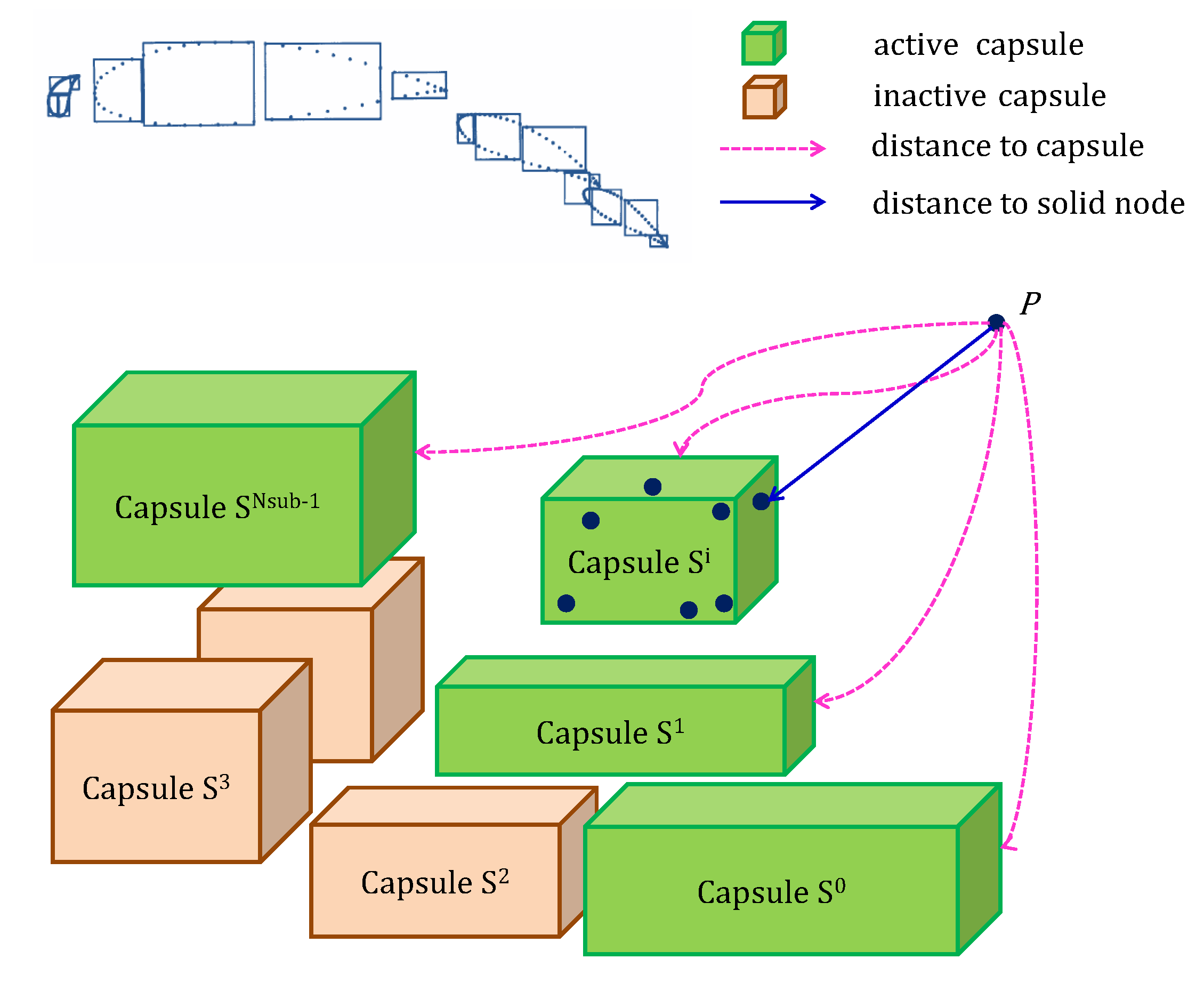
  • Calculate the distance from p to each cuboid capsule S i m . Figure 7 shows a schematic of d ( p , S i m ) , where the coordinates of p are ( x , y , z ) and the center of S i m is located at ( x c , y c , z c ) . The distance d ( p , S i m ) can be calculated as
    d ( p , S i m ) = f 2 ( x , x c , δ x ) + f 2 ( y , y c , δ y ) + f 2 ( z , z c , δ z )
    where
    f ( ξ , η , ζ ) = ξ η ζ 2 , i f ( ξ η ζ 2 ) , 0 , i f ( ζ 2 < ξ η < ζ 2 ) η ξ ζ 2 , i f ( ξ η ζ 2 )
    In addition, each cuboid capsule S i m has a property parameter indicating whether S i m is active and the initial value is set to TRUE. Note that d ( p , N w i ) is initialized to 10 40 .
  • Search for the cuboid capsule S i s that makes d ( p , S i s ) obtain its minimum among all the active cuboid capsules as shown in Figure 8. Whenever a suitable S i s is found, the index corresponding i s and d ( p , S i s ) are recorded. It is very likely that the capsule S i s contains the desired closest wall node, and a further verification is performed in Step 3. Otherwise, the routine goes directly to Step 4.
  • Update the value of d ( p , N w i ) as
    d ( p , N w i ) = min ( d ( p , N w i ) , d ( p , N w i s ) ) d ( p , N w i s ) = min ( d ( p , q ) q N w i s )
    and reset the property parameter of S i s to FALSE. If the cuboid capsule S i m satisfies the condition
    d ( p , S i m ) > d ( p , N w i )
    then its property parameter will be assigned to FALSE. The routine goes back to Step 2 and keeps on searching the active cuboid capsules.
  • After the above steps are completed, the smallest distance d ( p , N w i ) is obtained.
(c) Calculating ds and dt in parallel
As shown in Figure 6, p N i is an arbitrary node of source grid S G , and L target grids T G j ( 1 j L ) may overlap with S G . According to the domain decomposition strategy T 2 illustrated in Figure 3, S G can be treated with process-group P 0 and T G j with P j . The parameters d s and t s can be calculated as follows.
  • The solid wall nodes N w i of S G are collected and shared among processes in the group P 0 . Similarly, each process in P j also has the whole solid-wall nodes for component grid T G j .
  • All the processes calculate the distance d j ( 0 j L ) from p to the wall boundary in parallel.
  • Equation (7) indicates that d s is actually d 0 relevant to P 0 , and d t is the minimum of the L d j s.
Since the total number of solid wall nodes is much smaller than that of nodes on the whole grid, the current communication cost in the calculation of wall distance is greatly reduced compared to that of Ref. [12].

3.3.2. Verification Step: Parallel Treatment of Query Nodes

The query nodes N q i on grid G i can be defined as
N q i : = { p ( d t ( p ) < d s ( p ) ) ( p s = 0 L 1 B X j s ) }
where j s is the index of certain target grid of G i . Equation (15) only requires that the query node are covered by the minimal external box of the target grid, which is a necessary and insufficient condition for the coverage relation in Equation (2). Despite this, the treatment can exclude a large number of elements from the query nodes since the minimal external box can approximate the external boundary of the grid.
The ultimate goal of treating the query nodes is to identify the inactive nodes (Equation (2)). The parallel query algorithm and the relevant data stream are depicted in Figure 9. Assume the source grid G i is distributed in S processes with continuous indexes. In each process, an alternating digital tree (ADT) [26] is generated for the local grid, which provides fast-query services for any spatial node. Note that the query nodes belong to T index-continuous processes (different from the S processes hosting G i ), and each process contains a subset N q j s . Under the non-blocking communication pattern, the root process collects all the L subsets N q j s of query nodes and then broadcasts them to the S processors hosting the source grid G i . The parallel treatment of the query nodes is performed as follows:
  • Parallel query of donor cells and calculation of interpolation information. Each process hosting G i owns the whole query nodes N q i . On the help of the local ADT, we obtain the information whether an arbitrary query node p N q i is covered by any internal cell ε C i n i , i.e., p ε ˚ . If p ε ˚ holds, the information to be recorded includes the index of process containing ε , the local index of ε , the relative coordinates of p in ε , and d ( p , N w i ) . Otherwise, all the information relevant to p is erased from the current process.
  • Screening of query nodes. In each process relevant to G i , the information of query nodes is gathered by the collectors shown in Figure 9 and broadcasted to the T targeting processes. For an arbitrary node p N q j , if the stored process index is equal to that of current process P, then d t ( p ) is updated in the process P. Furthermore, if d t ( p ) < d s ( p ) holds, then p is an inactive node and excluded from N q j .
  • Classification of query nodes. After the above two steps, N q i may still contain inactive node. If p is covered by the minimal internal box of G i but no donor cells for p can be found on G i , then we treat p as an inactive node and remove it from N q j . Now all the remaining nodes in N q i are active.
Thus far, we have completed the parallelization of hole-cutting with the proposed two-step classification scheme. We utilize the distance parameters ( d s and d t ) and minimal external boxes to screen the query nodes, which can dramatically decrease the amount of nodes to be queried and thereby relieves the communication load of parallel computation.

3.4. Identification and Parallel Assembly of the Overlapping Cells

When the classification of nodes is accomplished, volume cells can be divided into flow-field cells, in-hole cells and overlapping cells according to the topological relation between cells and nodes. Most of the cells can be classified within the local process by applying a node-cell-coloring method. However, the interface between the transitional cells and inactive cells may coincide with the grid partition boundary surfaces (as shown in Figure 10). In this scenario, a point-to-point parallel communication at the boundaries is needed to transmit the cell information. The overlapping cells are identified as follows.
  • With the general method in Section 2.2, the cells are preliminarily divided into four categories, namely active cells, inactive cells, transitional cells and external overlapping cells (Figure 1).
  • All the nodes in the transitional cells are marked in a black colour, and these nodes are shared among all the processes.
  • In each process, the inactive cells containing black nodes are identified as interior overlapping cells, and the other inactive cells are classified as in-hole cells.
  • The interior overlapping and the external overlapping cells are unified into a set of overlapping cells. Similarly, the active cells and the transition cells are also unified into flow-field cells.

3.5. Treatment of Defective Cells

As shown in Figure 1, the overlapping cells come from the volume cells adjacent to the external boundary surfaces or from the inactive cells adjacent to the transitional cells. Equation (2) suggests that the lattice center of the latter case is displaced relative to the equidistance surface of different components. However, we may find some overlapping cells that cannot share strict coverage relation with the donor cells under certain conditions: (1) for a vanishing overlapping region, certain lattice centers of the overlapping cells may locate outside the overlapping regions; (2) when the gap between components is extremely narrow, the lattice centers of the overlapping cells may penetrate the solid wall boundary surfaces of the target grid. We call these overlapping cells defective cells.
To deal with the defective cells, proper mesh refinement of the overlapping regions can diminish the deviation of the overlapping cell centers, thereby reducing or even eliminating the defective cells. However, for the multi-body motion problems, the density of the mesh in the overlapping regions is difficult to control at each physical time step. Instead, we search the donor cells corresponding to the defective cells within an optimal grid-center distance. On the source grid G i , an extra layer of cells is constructed. Based on the minimal distance between the centers of overlapping cells and the extra-layer cells, we can obtain a single donor cell within the source grid.
  • On each process hosting the source grid G i , the donor cells for the relevant defective cells are independently selected.
  • In the non-blocking communication mode, the information about the above selected donor cells is gathered and then broadcasted to those processes (denoted by p t s) containing the distributed target grids.
  • In each process of p t s, the defective cells are independently screened, and the nearest flow-field cells are taken as donor cells.
On completion of treating the defective cells, full information of the overlapping assembly can be provided to the numerical simulator.

4. Implementation and Application of Overlapping-Grid-Sewing-Machine Library

The proposed parallel implicit assembly method in Section 3 has been realized into the overlapping grid sewing machine (OGSM) library based on the message passing interface (MPI) standard and C++ programming language. We hereby give an introduction to the data ferry technique, the application programming interfaces (APIs) to simulators and the relevant work-flow.

4.1. Data Ferry Technique

In the parallel implementation of OGSM, the nodes and cells of component grids are all distributed throughout multiple processes. Even within the same process, the memory space of these objects is generally discontinuous, owing to the memory allocation convention of C++. However, there are scenarios where the complete geometric information is needed by the relevant processes. For instance, all the solid-wall nodes are needed in the calculation of the wall-distance parameters (Equation (1)), and the dispersed query nodes should be gathered to perform the cross-process searching operations. Consequently, we construct a data ferry using C++ to deal with the cross-process packaging and sharing of dispersed data, which can significantly reduce the overall frequency of data transmission.

4.1.1. Customized Data Packaging Type

For the C++ programming language, the data members of arbitrary type can be decomposed into basic types. Furthermore, the data of basic types and that of the general binary type can be converted to each other. We define a data structure named DataUnit to carry binary data with a dynamic vector, i.e., vector〈char〉 data in the C++ Standard Template Library. We also wrap the non-blocking MPI functions to transfer the DataUnit objects.
The maximal length of data in a single communication (denoted by m s z ) is limited by the MPI functions, which makes a single DataUnit object inadequate for messages of large-scale parallel computing. To deal with this, a threshold d u s z controlling the maximal length of data contained in the DataUnit object is set to a value not exceeding m s z . For large data whose length is larger than d u s z , multiple DataUnit objects are generated and linked in sequence to form a DataStream, as shown in Figure 11a. Note that the total number of the DataUnit objects in each DataStream may vary the data volume.

4.1.2. Data Ferry

In addition to using the DataStreams to solve the problem for large-scale data transmission, we further introduce the concept of a data ferry, which is integrated into our OGSM library. The top part of Figure 11b denotes the processes related to the source grids, whose ranks are represented with { i 0 , i 1 , , i S 1 } . They send messages to the processes for the target grids T G (bottom), which are represented by ranks { j 0 , j 1 , , j T 1 } . Concretely speaking, the work-flow for data ferry is as follows:
  • Each process p i m ( m [ 0 , S 1 ] ) creates a DataStream object and sends the collected data to the root process p i 0 .
  • Process p i 0 receives the messages from S DataStream objects and gathers them into a collector of the pointer object.
  • The information in collector is broadcasted to the processes p j n ( n [ 0 , T 1 ] ) . When the sender p i m and the receiver p j n are the same process, a memory-copy operation is called instead to replace the MPI communication.

4.2. Application Programming Interfaces for Simulators

OGSM provides convenient interfaces for its integration into CFD simulators. Section 4.2.1 presents the parameters of boundary conditions in the controlling file, and Section 4.2.2 introduces the functions for grid topology.

4.2.1. Controlling Parameters of Boundary Conditions

Table 1 lists the four controlling parameters of boundary conditions (BCs) stored in a file named “overset.txt”. OGSM utilizes solidWBC and externalBC to handle the solidwall and external boundary conditions for different components grids. When all these parameters are assigned, OGSM can automatically identify the boundaries of the overlapping grids.

4.2.2. Input and Output Interfaces

OGSM can be easily integrated into other CFD simulators by calling the ImportData (Figure 12) and ExportInfo (Figure 13) functions.
Table 2 lists all the parameters of ImportData. It can be seen that users should provide four types of information, namely domain decomposition, grid points, adjacency relationship and boundary conditions.
Similarly, Table 3 lists the five parameters of function ExportInfo, which represent the assembly results of overlapping grids. sourceRankList denotes the indexes of processes owing interpolation cells, while sourceCellList and targetCellList show the local indexes of interpolation and donor cells in their processes. lagrangeFactor records the interpolation coefficients of each point to the corresponding donor cell, and iblank describes the types of all cells, i.e., flow-field cells, in-hole cells and overlapping cells.

4.3. Internal Work-Flow of OGSM Library

As shown in Figure 14, the internal work-flow of OGSM can be divided into 12 basic steps:
  • Import the topology information of the grid distribution in the current process, including the sequence of the spatial nodes, faces and cells. The boundary conditions and the cross-process adjacency relationship between grids are simultaneously attached.
  • Recognize solid wall and external boundaries. According to the solidWBC and externalBC parameters assigned by users in “overset.txt”, a quick mapping is performed to identify the solid wall and external boundaries of grids.
  • Register face-to-face adjacency relationship. Note that the internal overlapping cells are obtained by extending the transitional cells towards the inactive cells, which may require certain cross-process operations. Therefore, we register the face-to-face adjacency relationship of the sub-grids based on the geometric information obtained in step 1.
  • Record the overlapping relationship between multiple component grids. According to the spectral analysis results of the covariance matrix, the minimal internal and external boxes of component grids can be generated in parallel. Then, a spatial planeseparation algorithm is utilized to preliminarily determine the overlapping relation between component grids.
  • Initialize the query nodes via the preliminary screening criterion. The recursive-box algorithm is used for the parallel calculation of wall distance parameters d s and d t . The query nodes are preliminarily screened according to the distance relation and the coverage relation.
  • Update the ADT structures corresponding to the sub-grids. Both the inspection of the coverage relation in Equation (2) and the pairing between overlapping cells and donor cells require cross-process searching. Compared to the traditional recursive query mode, the non-recursive query of ADTs utilized in OGSM can improve the query speed on the ADTs and avoid the stack-overflow effects caused by the large tree structures [27].
  • Confirm the types of query nodes. The coverage relationship is judged based on ADT, and the inactive query nodes are excluded. Note that the properties of the nodes to be queried are screened in parallel.
  • Classify global volume cells. The hole-cutting boundaries are determined and the global volume cells are classified into flow-field cells, overlapping cells and in-hole cells.
  • Query the optimal donor cells for overlapping cells. The tri-linear interpolation coefficients are calculated in parallel. For defective overlapping cells, the recursive-box method is adopted to quickly search for the optimal donor cells, and the other overlapping cells are paired to their donor cells by applying cross-process searching on ADT structures and the Newton–Raphson iterative method.
  • Treat the assembly information in parallel. The mapping ( i p , i d ) ( j p , j d , f s ) holds for any overlapping cell in each process. Hereby, i p and i d represent the process index and local cell index of the current overlapping cell on the source grid. Meanwhile, j p , j d , and f s represent the process index, the local cell index and the interpolation factors of the corresponding donor cell on the target grid, respectively. Then, the target processes prepares the data for interpolation based on the mapping.
  • Count the total number of donor cells in the current process. Strictly speaking, this value is equal to the total number of interpolation operations in the current process. For an unsteady flow field with multi-body relative motion, the assembly state of the overlapping grids changes at each physical time step. Meanwhile, the total number of donor cells on each process varies. OGSM provides the solver with this critical parameter, which enables it to dynamically manage the memory space and perform the interpolation of the physical field.
  • Export the information of overlapping interpolation and cell classification. First, the current process outputs the overlapping relations; then the solver interpolates the physical field using the tri-linear factors and exchanges the data across processes for the donor cells. Finally, the type identifiers of volume cells are outputted as an iBlank value (0: in-hole, 1: overlapping, 2: flow-field).
OGSM consists of three modules, i.e., the topology generation module of overlapping grids (steps 1 to 3), the parallel hole-cutting module (steps 4 to 7) and the parallel assembly module for overlapping cells (steps 8 to 11).

5. Numerical Results

5.1. Assembly for a Seven-Ball Configuration

To test the capability of OGSM in the parallel assembly of overlapping multi-component grids, we applied it to a seven-sphere model, as shown in Figure 15. Unstructured grids were generated independently for each sphere component, with the geometric center coinciding with that of the respective sphere. The overlapped grids have 36,085,811 nodes and 211,912,897 volume cells in total. Each of the seven components has 4,989,826 nodes and 29,256,824 cells, while the background grid has 6,146,855 nodes and 36,371,953 cells. The overlapping grids were assembled in parallel with 32, 64, 128, 256, 512 and 1024 processes, and the relevant computation time is listed in Table 4.
Figure 16 presents a slice of the overlapping cells and flow-field cells on the z = 0 plane for 1024 processes. It shows an automatic assembly of seven grid areas. The blue curve represents the grid-partition boundary, and the green part is the overlapping cells. In this example, the external boundary of the component grid intersects with the hole-cutting boundary, which follows the wall distance criterion.
Figure 17 demonstrates the wall-time curves as a function of the total number of processes for each OGSM sub-module, i.e., Figure 17a for calculating the wall-distance parameters, Figure 17b for the ADT generation, Figure 17c for the parallel identification of the node properties, and Figure 17d for the pairing between the overlapping cells and donor cells.
Figure 18 shows the wall-time curve of the entire assembling operation of the overlapping grid using OGSM for an increasing number of the processors. It can be observed that OGSM possesses a high level of parallelization, which shows its potential to deal with large-scale geometry data even under high workloads for each process. Moreover, each process can quickly generate the ADT structure related to the grids in negligible time. Finally, there are three steps which occupy over 95 % of the total time, i.e., the calculation of the wall distance parameters, the parallel identification of the properties of preliminary screened nodes, and the pairing of overlapping cells and donor cells.
Figure 17c,d suggests that when the total number of processes does not exceed 512, the time consumptions of both the hole-cutting and the pairing between overlapping cells and the donors monotonically decrease. This is because a decrease in the average load leads to a decrease in the depths of the ADTs, thereby lessening the average time for searching. However, the size of the query nodes set or the overlapping cells set on the entire grids cannot be reduced by increasing the total number of processes. In other words, the amount of data collected and shared among the processes remains unchanged. At this moment, the frequency of data sharing increases. Accordingly, the time consumption is dominated by the communication. In Figure 17d, when the total number of processes reaches 1024, the time consumption by the pairing of the overlapping cells and the donor cells slightly increases.
Notwithstanding, by comparing Figure 17c with Figure 17d, it can be observed that the difference in the time consumption under the same number of processes is negligible. In this example, the size of the query nodes set is close to that of the overlapping cells. The decoupled analysis model based on distance relation and coverage relation has greatly reduced the size of query nodes set within the spatial range. (Note: the query nodes set in reference [12] includes all nodes on the grids, which far outnumber the overlapping cells near the equidistant surfaces between different components).

5.2. A Multiple Body Trajectory Prediction Case Study

In order to further verify the accuracy of the interpolation for the overlapping cells, we embedded OGSM into an in-house flow field solver named “parallel simulator for multi-block grids in three-dimensional space” (PMB3D) [28] in the form of a static library and performed a simulation for the unsteady field of a case containing three external objects.
Figure 19 shows the geometry configuration of this case study, which stems from the “multiple body trajectory prediction” (MBTP) model. Interested readers can refer to the literature [29,30] for more information.
Multi-block structured grids were generated around the wing and external objects. The wing grid has 5,214,792 nodes and 4,798,080 cells, and each external object has 1,722,242 nodes and 1,585,664 cells. Consequently, the total number of nodes and cells for the MBTP configuration are 10,291,518 and 9,555,072, respectively.
To the best of our knowledge, there are no convincing wind tunnel experimental results for the multiple body trajectory prediction case. Consequently, we merely performed the numerical simulation with 64 processes. In each process, the coincident nodes and faces were merged, and the multi-block structured grids were transformed to an independent unstructured grid. When the overlapping assembly was accomplished by OGSM, the PMB3D performed the simulation of the Reynolds-averaged Navier–Stokes (RANS) equation. The convection and the viscosity terms were approximated with the Roe scheme and the SA turbulence model, respectively. A dual time-step approach was employed in the time direction. To suppress the unphysical results, a minmod limiter was included. The Mach number of the free stream was set to 0.95 . The lower external object was dropped at first, followed by the upper-left one in 0.04 s and the upper-right after another 0.04 s. The ejection force applied to the store at the bottom was vertically downward, while the one at the shoulder was 45 degrees from the vertical and points outward. The action time was 0.045 s.
Figure 20 shows the hole-cutting effect of each component grid obtained by OGSM for a cross-section perpendicular to the x-axis. The red part is the flow field domain, the yellow part is the automatic hole-cutting boundary, and the green part is the overlapping cells. It can be seen that OGSM successfully realized the cutting and connection of the flow field area for each component.
Figure 21 shows the variation trend of the trajectory and the attitude of the three external objects within 0.51 s. A yaw motion from the head of the external object(s) towards the wing tip can be observed. At the initial stage, the ejection force exerted on the head and the tail of the external object(s) forms a head-up moment. This moment is then cancelled by the stabilization effect of the tail. In the numerical simulation, the ejection force is applied on the body shaft system fixed to the external object, such that no rolling moment is generated.
Figure 22a–c show the temporal variation of the centroid trajectory, and Figure 22d–f show the attitude angles (rolling angle Φ , pitch angle Θ and yaw angle Ψ ) for the three objects, respectively. The centroid trajectory obtained by the simulation agrees well with that from the Refs. [29,30], whereas the prediction of the attitude angles still yields certain non-negligible errors.
In this example, the errors mainly come from the physical field interpolation of the overlapping cells. On the one hand, by tracking the execution of OGSM, some defective overlapping cells are detected during the implicit hole-cutting. Taking the initial status as an example, the total number of the defective overlapping cells in the whole domain is 61. On adopting the fault tolerant mechanism, the donor cell (the cell at the sub-layer) fails to cover the geometric center of the current defective overlapping cell. In this case, the interpolation cannot be strictly performed inside the donor cell, which reduces the local precision. On the other hand, compared to the steady numerical simulation, the unsteady flow field imposes higher requirements for the conservation of the numerical format (as analyzed by Borazjani [11]). Although linear interpolation guarantees the robustness of the discretization scheme, the resulting errors exhibit a cumulative effect over time. These factors mutually lead to the observable errors of the multi-body trajectory in the later stage. In the future, we will try to expand the template of the donor cells and construct certain conservative interpolation schemes to improve the accuracy of unsteady numerical simulation on the overlapping grids.

6. Conclusions

The traditional implicit assembly techniques for overlapping grids usually search grid nodes in an undifferentiated manner, which can result in low parallel assembly efficiency. To address this issue, we have proposed an efficient parallel overlapping grid implicit assembly algorithm employing a two-step node classification scheme to accelerate the hole-cutting operation. Further more, we have implemented the proposed method into the OGSM library ready for integration by other CFD solvers. We have verified the parallel assembly capability of OGSM with a seven-sphere configuration, and the relevant experimental results demonstrate that OGSM shows good scalability in dealing with large-scale geometry data. We have also validated the parallel computing efficiency and interpolation accuracy of OGSM with a multi-body dropping case.
Future work will include the following three aspects. First, in order to improve the simulation quality of flow field details, the adaptive Cartesian grids will be combined with the overlapping assembly methods for structured/unstructured grids based on a unified software framework. Second, the conservative interpolation method for the overlapping cells will be comprehensively investigated to meet the requirements of unsteady numerical simulations. Last but not least, a more stringent preliminary screening technology will be studied to improve the efficiency in assembling large-scale overlapping grids.

Author Contributions

Conceptualization, Y.G. and X.J.; methodology, Y.G.; software, F.L. and Y.G.; validation, B.Z., B.C. and Z.W.; formal analysis, Z.W. and Z.X.; investigation, F.L. and Y.G.; resources, B.Z., B.C. and Z.W.; writing—original draft preparation, F.L. and Y.G.; writing—review and editing, B.Z.; visualization, Z.W., B.C. and Z.X.; supervision, X.J.; project administration, X.J.; funding acquisition, F.L. and X.J. All authors have read and agreed to the published version of the manuscript.

Funding

This work was partly supported by the Science and Technology Innovation 2030 Major Project under grant no. 2020AAA0104801, the Natural Science Foundation of China under grant no.61903364, Scientific Research Projects under grant no. JK20211A010103 and the National Numerical Windtunnel Project.

Institutional Review Board Statement

Not applicable.

Informed Consent Statement

Not applicable.

Data Availability Statement

Data sharing not applicable.

Acknowledgments

The authors would like to thank Yiou Liu and Markus Müllner from RWTH Aachen University for proofreading the manuscript.

Conflicts of Interest

The authors declare no conflict of interest.

References

  1. Yang, C.; Xue, W.; Fu, H. 10M-Core Scalable Fully-Implicit Solver for Nonhydrostatic Atmospheric Dynamics. In Proceedings of the International Conference for High Performance Computing, Networking, Storage and Analysis, Salt Lake City, UT, USA, 13–18 November 2016; pp. 1–12. [Google Scholar]
  2. Deng, S.; Xiao, T.; van Oudheusden, B.; Bijl, H. A dynamic mesh strategy applied to the simulation of flapping wings. Int. J. Numer. Methods Eng. 2016, 106, 664–680. [Google Scholar] [CrossRef]
  3. Li, Y.; Paik, K.; Xing, T.; Carrica, P. Dynamic overset cfd simulations of wind turbine aerodynamics. Renew. Energy 2012, 37, 285–298. [Google Scholar] [CrossRef]
  4. Lu, C.; Shi, Y.; Xu, G. Research on aerodynamic interaction mechanism of rigid coaxial rotor in hover. J. Nanjing Univ. Aeronaut. Astronaut. 2006, 51, 201–207. [Google Scholar]
  5. Fan, J.; Zhang, H.; Guan, F.; Zhao, J. Studies of aerodynamic interference characteristics for external store separation. J. Natl. Univ. Def. Technol. 2018, 40, 13–21. [Google Scholar]
  6. Steger, J.; Benek, J. On the use of composite grid schemes in computational aerodynamics. Comput. Methods Appl. Mech. Eng. 1987, 64, 301–320. [Google Scholar] [CrossRef]
  7. Meakin, R.; Suhs, N. Unsteady aerodynamic simulation of multiple bodies in relative motion. In Proceedings of the 9th Computational Fluid Dynamics Conference, Buffalo, NY, USA, 13–15 June 1989; p. 1996. [Google Scholar]
  8. Vreman, A. A staggered overset grid method for resolved simulation of incompressible flow around moving spheres. J. Comput. Phys. 2017, 333, 269–296. [Google Scholar] [CrossRef]
  9. Steger, J.; Dougherty, F.; Benek, J. A Chimera grid scheme. Adv. Grid Gener. ASME 1983, 5, 59–69. [Google Scholar]
  10. Meakin, R. Object X-rays for cutting holes in composite overset structured grids. In Proceedings of the 15th AIAA Computational Fluid Dynamics Conference, Anaheim, CA, USA, 11–14 June 2001; p. 2537. [Google Scholar]
  11. Borazjani, I.; Ge, L.; Le, T.; Sotiropoulos, F. A parallel overset-curvilinear-immersed boundary framework for simulating complex 3d incompressible flows. Comput. Fluids 2013, 77, 76–96. [Google Scholar] [CrossRef] [Green Version]
  12. Lee, Y.L.; Baeder, J. Implicit Hole Cutting—A New Approach to Overset Grid Connectivity. In Proceedings of the 16th AIAA Computational Fluid Dynamics Conference, Orlando, FL, USA, 23–26 June 2003. [Google Scholar]
  13. Liao, W.; Cai, J.; Tsai, H. A multigrid overset grid flow solver with implicit hole cutting method. Comput. Methods Appl. Mech. Eng. 2007, 196, 1701–1715. [Google Scholar] [CrossRef]
  14. Nakahashi, K.; Togashi, F.; Sharov, D. An Intergrid-boundary definition method for overset unstructured grid approach. AIAA J. 2000, 5, 2077–2084. [Google Scholar] [CrossRef]
  15. Togashi, F.; Ito, Y.; Nakahashi, K.; Obayashi, S. Extensions of Overset Unstructured Grids to Multiple Bodies in Contact. J. Aircr. 2006, 43, 52–57. [Google Scholar] [CrossRef]
  16. Landmann, B.; Montagnac, M. A highly automated parallel Chimera method for overset grids based on the implicit hole cutting technique. Int. J. Numer. Methods Fluids 2011, 66, 778–804. [Google Scholar] [CrossRef]
  17. Meakin, R.; Wissink, A. Unsteady aerodynamic simulation of static and moving bodies using scalable computers. In Proceedings of the 14th AIAA Computational Fluid Dynamics Conference, Norfolk, VA, USA, 1–5 November 1999; p. 3302. [Google Scholar]
  18. Belk, D.; Maple, R. Automated assembly of structured grids for moving body problems. In Proceedings of the 12th AIAA Computational Fluid Dynamics Conference, San Diego, CA, USA, 19–22 June 1995; pp. 381–390. [Google Scholar]
  19. Suhs, N.; Rogers, S.; Dietz, W. PEGASUS 5: An Automated Pre-Processor for Overset-Grid CFD. AIAA J. 2013, 45, 16–52. [Google Scholar]
  20. Noack, R.W.; Boger, D.A. Improvements to SUGGAR and DiRTlib for overset store separation simulations. In Proceedings of the 47th AIAA Aerospace Science and Exhibit, Orlando, FL, USA, 5–8 January 2009. [Google Scholar]
  21. Noack, R.W.; Boger, D.A.; Kunz, R.F.; Carrica, P.M. Suggar++: An improved general overset grid assembly capability. In Proceedings of the 47th AIAA Aerospace Science and Exhibit, Orlando, FL, USA, 5–8 January 2009. [Google Scholar]
  22. Roget, B.; Sitaraman, J. Robust and Scalable Overset Grid Assembly for Partitioned Unstructured Meshes. In Proceedings of the 51th AIAA Aerospace Science and Exhibit, Grapevine, TX, USA, 7–10 January 2013. [Google Scholar]
  23. Hedayat, M.; Akbarzadeh, A.M.; Borazjani, I. A parallel dynamic overset grid framework for immersed boundary methods. Comput. Fluids 2022, 239, 105378. [Google Scholar] [CrossRef]
  24. Chang, X.H.; Ma, R.; Zhang, L.P. Parallel implicit hole-cutting method for unstructured overset grid. Acta Aeronaut. Astronaut. Sin. 2018, 39, 121780. [Google Scholar]
  25. Bergen, G.V.D. A Fast and Robust GJK Implementation for Collision Detection of Convex Objects. J. Graph. Tools 1999, 4, 7–25. [Google Scholar] [CrossRef]
  26. Bonet, J.; Peraire, J. An alternating digital tree (ADT) algorithm for 3D geometric searching and intersection problems. Int. J. Numer. Methods Eng. 1991, 31, 1–17. [Google Scholar] [CrossRef]
  27. Crabill, J.; Witherden, F.D.; Jameson, A. A parallel direct cut algorithm for high-order overset methods with application to a spinning golf ball. J. Comput. Phys. 2018, 374, 692–723. [Google Scholar] [CrossRef] [Green Version]
  28. Ma, S.; Qiu, M.; Wang, J.T. Application of CFD in slipstream effect on propeller aircraft research. Acta Aeronaut. Astronaut. Sin. 2019, 40, 1–15. [Google Scholar]
  29. Prewitt, N.C.; Belk, D.M.; Maple, R.C. Multiple-Body Trajectory Calculations Using the Beggar Code. J. Aircr. 1999, 36, 802–808. [Google Scholar] [CrossRef]
  30. Davis, D.C.; Howell, K.C. Trajectory evolution in the multi-body problem with applicationsin the Saturnian system. Acta Astronaut. 2011, 69, 1038–1049. [Google Scholar] [CrossRef]
Figure 1. Relationship between cell sets.
Applsci 12 07804 g001
Figure 2. Schematic illumination of overlapping grids.
Applsci 12 07804 g002
Figure 3. Comparison of two partition strategies.
Applsci 12 07804 g003
Figure 4. Overlapping relationship of the propeller blade mesh.
Applsci 12 07804 g004
Figure 5. Schematic diagram of spatial separation plane algorithm.
Applsci 12 07804 g005
Figure 6. Illustration of distance from a given node to solid wall boundaries.
Applsci 12 07804 g006
Figure 7. Schematic diagram of distance from a given node to a cuboid capsule.
Applsci 12 07804 g007
Figure 8. Diagram of recursive-box algorithm for wall distance calculation.
Applsci 12 07804 g008
Figure 9. Node query algorithm and interpolation information.
Applsci 12 07804 g009
Figure 10. Partial coincidence between hole-cutting boundaries and partition boundaries.
Applsci 12 07804 g010
Figure 11. Construction of data package and data ferry.
Applsci 12 07804 g011
Figure 12. Input interface for grid topology.
Applsci 12 07804 g012
Figure 13. Output interface for assembly results.
Applsci 12 07804 g013
Figure 14. Internal work-flow of OGSM library.
Applsci 12 07804 g014
Figure 15. Seven sphere components.
Applsci 12 07804 g015
Figure 16. Slice through overlapping cells and field cells (z = 0, 1024 processes).
Applsci 12 07804 g016
Figure 17. Wall time curves for different parallel assembly steps of a 7 spherical parts grid.
Applsci 12 07804 g017
Figure 18. Total wall time for parallel assembly of a 7 spherical parts grid with growing number of processes.
Applsci 12 07804 g018
Figure 19. Grid topological structure of the example of continuous delivery of external stores.
Applsci 12 07804 g019
Figure 20. Overlapping grid hole-cutting effect for multi-component configuration.
Applsci 12 07804 g020
Figure 21. Trajectory and posture change trend of external objects.
Applsci 12 07804 g021
Figure 22. Centroid trajectories and attitude angles of the external stores.
Applsci 12 07804 g022
Table 1. Controlling parameters for boundary conditions.
NameTypeDescription
numOfSolidWBCintthe number of solid-wall BC identifiers
solidWBC[ ]int arraythe solid-wall identifiers
numOfExtBCintthe number of external BC identifiers
externalBC[ ]int arraythe external BC identifiers
Table 2. Parameters of input interface for grid topology.
NameTypeDescription
zoneIndexSpanint*number of processes for each component grid
numberOfGridGroupsintnumber of component grids
xx, yy, zzdouble*coordinates of grid points in current process
numberOfNodesintnumber of grid points in current process
faceToCellRelationint*relationship between two adjacent cells
physicalTypeint*boundary condition types for faces
numberOfNodesOnFaceint*number of grid points on each face
nodeIndexListOnFaceint*list of node indexes on face
numberOfFacesintnumber of faces on current process
geometricTypeint*type of volume cells in current process
faceIndexListint*list of face indexes around cells in current process
numberOfCellsintnumber of cells in current process
outerZoneListint*list of processes owing dual face at border
outerFaceListint*local indexes of dual faces at border
numberOfOuterFacesintnumber of dual faces at domain decomposition border
numberOfPhysicalFacesintnumber of physical faces excluding dual faces
Table 3. Parameters of output interface for assembly results.
NameTypeDescription
sourceRankListint*index of process owing interpolation cells
sourceCellListint*local index of interpolation cells in their processes
targetCellListint*local index of donor cells in their processes
lagrangeFactordouble*lagrange interpolation factors
iblankint*type of cells in current process
Table 4. Computation time in seconds of assembly subroutine for different processes.
Subroutine32P64P128P256P512P1024P
ReadGeometry19.4031.0121.848.5413.750.78
RegContactRel53.4028.984.913.503.976.34
RegOversetRel3.090.980.570.370.330.20
CalWallDist903.95458.84289.34114.7670.6137.71
ExOutQryNode0.190.210.020.000.020.00
GenBgrdTree36.8526.2912.564.571.931.00
ConfrmQryNode368.37217.68185.73118.5072.2762.23
ClassifyElems2.401.710.830.370.180.06
AssemblyElems215.92154.91124.1976.9559.2063.28
SewingGrid2.113.233.706.3811.8423.10
WritingFile169.50115.22160.07148.76148.66138.09
TotalTime1775.181039.06803.76482.70382.76332.79
Publisher’s Note: MDPI stays neutral with regard to jurisdictional claims in published maps and institutional affiliations.

