An Intelligent Weighted Object Detector for Feature Extraction to Enrich Global Image Information

Abstract

Object detection is a fundamental task in computer vision. To improve the detection accuracy of a detection model without increasing the model weights, this paper modifies the YOLOX model by first replacing some of the traditional convolution operations in the backbone network to reduce the parameter cost of generating feature maps. We design a local feature extraction module to chunk the feature maps to obtain local image features and a global feature extraction module to calculate the correlation between feature points to enrich the feature, and add learnable weights to the feature layers involved in the final prediction to assist the model in detection. Moreover, the idea of feature map reuse is proposed to retain more information from the high-dimensional feature maps. In comparison experiments on the dataset PASCAL VOC 2007 + 2012, the accuracy of the improved algorithm increased by 1.2% over the original algorithm and 2.2% over the popular YOLOv5.

1. Introduction

From the improvement of network performance [1,2] to the authentication of personal identity in the Internet of Things [3], the real-time sensing of vehicle queue length, pedestrian detection [4,5], and research on facial expression recognition [6] in smart cities, artificial intelligence as a combination of different fields has penetrated all aspects of people’s lives. With the continuous progress of artificial intelligence, computer vision has become a focus in the field of artificial intelligence, and object detection, as the cornerstone of computer vision, is the basis for solving more complex and higher-level vision tasks such as segmentation, scene understanding, object tracking, image description, temporal detection, and activity recognition, providing the basic information requirements for computer vision applications to detect the class to which an object in a digital image belongs, such as cars, bicycles, airplanes, etc. Computer vision is widely applied in the fields of intelligent transportation, human-computer interaction, and autonomous driving [7]. Meanwhile, object detection in the field of smart agriculture is being implemented by drones for real-time detection of field crops and to allow the timely detection of field weeds and spraying of herbicide drugs [8].

With the rapid development of deep learning concepts, object detectors can now be categorized into four types: (1) two-stage object detectors, such as VFNet [9] and CenterNet2 [10], which are generally better than single-stage detectors, but are slightly less real-time; (2) single-stage object detectors, e.g., YOLOX [11] and DETR [12], which improve the detection rate of two-stage detection, though their detection accuracy is decreased slightly; (3) anchor-based detection, such as YOLOv5 [13], which often requires setting multiple anchor sizes in advance and can effectively improve network target recall, but requires strong a priori knowledge; and (4) anchor-free detectors, e.g., RepPoints [14] and YOLOX [11], which do not require the artificial setting of anchor sizes and eliminate the computational effort of anchor-based methods, but sometimes have unstable detection effects.

At present, object detection algorithms are widely used in real-world scenarios such as drone driving, intelligent transportation, and automatic driving. However, despite their application, existing object detection algorithms still have the following problems:

• The images input to neural networks are often multiscale, so object detectors cannot achieve the desired performance. Even two-stage object detection algorithms have difficulty in extracting finer-grained features;
• The deep convolutional layer integrates the features extracted from the bottom convolutional layer, so the deeper the network is, the richer the global feature information, but more convolutional layers result in the loss of more detailed information;
• Higher-level features correspond to larger receptive fields and can obtain global information about the instance, such as pose. Lower-level features retain better location information and can provide finer details. It is a constant problem in object detection to adopt an effective feature fusion method to fuse the semantic information between different layers.

In this paper, to address the above problems in object detection, based on YOLOX [11], a cheaper convolution method replaces a part of the convolution method of the backbone network in the model to obtain image features, which reduces the extracted feature parameters in the model. In order to obtain more fine-grained features, a local feature extraction module is added to the middle layer of the backbone network. Considering the abundance of global information in the deeper layers, global feature modules are added to the deeper convolution layers to reduce the loss of global information during the convolution process. To add weights to the features from different layers and let the model learn the contribution of features from different layers, the idea of “feature map reuse” is proposed. This solves the shortcoming of introducing a large number of convolution parameters to adjust the channel dimension when summing up the feature maps from different layers; i.e., the dimension can be improved without adding any parameters.

Therefore, the main contributions of this paper are as follows:

• Replacing the common 3 × 3 convolutional approach in the backbone network CSPdarknet53 to extract features of images with fewer parameters, making the backbone network more efficient in extracting features;
• Designing local extracted feature modules so that different regions on the feature map receive the attention of different convolution kernels to extract fine-grained features;
• Introducing a global feature extraction module in the deep convolutional layer in which the semantic correlation of any two points in the feature map is calculated, thereby weakening the feature points with insufficient semantic information, compensating for the lack of global information ignored by the convolutional operation, and providing richer global feature information for the later layers or the final detection;
• In the feature fusion part of the model, multiscale fusion can assist the model for better performance detection, while giving weights to different layers of the model, i.e., adding a simple self-learning attention mechanism that makes the model focus more on the feature layers with a larger proportion of weights;
• This paper proposes a new method to enhance the dimension of the channel, which reuses the generated feature map and retains more original information about the image without using convolution.

In the structure of this paper, Section 2 describes the developments in the field of object detection, Section 3 introduces the GhostNet model and non-local neural networks, Section 4 presents the improved model in this paper, Section 5 shows the experimental results and the analysis of the results, and Section 6 provides a summary of the work in this paper.

2. Related Work

Feature extraction by convolution: In image feature extraction, the traditional method is generally divided into three steps: pre-processing, feature extraction, and feature processing. Finally, machine learning and other methods are utilized to classify the features and other operations. The purpose of image pre-processing is mainly to eliminate interference factors and highlight feature information; the main method used is image normalization. Traditional feature extraction mainly uses feature extractors to extract features from images, such as the SIFT algorithm, which is commonly used in the field of image matching. It can maintain invariance for rotation, scale scaling, and changes in brightness, and is highly resistant to occlusion, but it is computationally intensive. The HOG algorithm for pedestrian detection, although it reduces the dimensionality of the representation data needed for images, has poor real-time performance [15].

Since the rise of deep learning, convolutional neural networks have gradually replaced manual feature extraction methods. Generative adversarial networks generate similar images by learning the distribution of original image data and consist of a generator and a discriminator [16], while convolutional neural networks learn data features and extract beneficial information from them. A properly designed convolutional network can bring qualitative changes to model detection performance. DenseNet [17] achieves the ultimate utilization of features to achieve better network results with fewer parameters. The lightweight network MobileNet [18,19] is a lightweight deep neural network proposed by Google for embedded devices such as cell phones. Its core idea is deep separable convolution, which greatly reduces the parameters of convolution in the model. In the ShuffleNet series [20,21], pointwise group convolution and random channel shuffle are used to achieve a balance between model detection speed and accuracy, making it possible to deploy this network with low latency on the mobile side. EfficientV1 [22] explores the relationship between input resolution and network depth and width, and achieves a balance of the three dimensions according to the scaling provisions, while EfficientV2 [23] introduces the Fused-NBConv module and a progressive learning strategy based on EfficientV1 while employing a non-uniform scaling strategy to adjust the model size. ResNeSt [24] uses multiple convolutional kernels in the same layer to extract features separately, while introducing a soft attention mechanism to achieve weight distribution among feature channels, and finally proposes a modular split-attention block. In GhostNet [25], there are many redundant feature maps in the high-dimensional feature maps generated deep in the network, so an inexpensive convolution operation is designed to generate feature maps of equal channels and build a lightweight network. A sparse feature reactivation method is proposed in CondenseNet V2 [26], where each convolutional layer can selectively reuse the most important features from the previous layer and update the features in the previous layer to achieve the utility of the updated feature layer. In the case of ReXNet [27], it was argued that excessive reduction in the size of the feature map may lead to information loss and cause problems of degraded model performance, so Han et al. conducted an in-depth study of the rank of the feature matrix generated by a variety of random networks and designed a more accurate network structure that moderates the side effects of representative bottlenecks.

Global information of the feature: Global features describe the overall attributes of an image, including color features, texture features, and shape features. Local features are features extracted from local regions of an image, including edges, corner points, lines, curves, and areas of specific attributes. In recent years, local image features have been widely applied in face recognition, 3D reconstruction, and target recognition and tracking. Wang et al. proposed MGN [28] to uniformly divide an image into multiple strips and vary the number of parts in different local branches to obtain local feature representations with many granularities. The Local Relation Networks [29] propose a local network that can fuse the feature maps of multiple channels that express the same information, improving the representation of the neural network with the same number of channels.

Stacked convolutional layers can synthesize the local information obtained from the underlying layers to obtain richer global features. However, the more convolutional layers the feature map goes through, the more significant the loss of global information will be. Non-local neural networks [30] focus on the correlation between each pixel point on the image to obtain global information. In recent years, various transformer-based models have emerged due to the global character of transformers. The first one is DETR [31], which successfully integrates a transformer into the object detection model, simplifies the detection process, and outputs the set of prediction results directly in an end-to-end manner. Inspired by MobileNet and transformers, Microsoft proposed a mobile-former for the parallel design of MobileNet and a transformer [32], that is, to establish a bidirectional bridge between MobileNet and a transformer. Thus, convolution and a vision transformer are combined to realize the bidirectional fusion of local and global features. In view of the imbalance between foreground and background and the serious loss of global information in object detection, Tsinghua and Byte proposed FGD [33], which separates foreground and background using focal distillation while instructing students in knowledge distillation by using teachers’ spatial and channel attention as pre-training weights, as well as using the proposed global distillation to extract global information from students and teachers separately. Considering the importance of the receiver domain in the feature extraction network, LoFTR [34] borrows the self-attention and mutual-attention layers from a transformer to obtain feature descriptions between images and proposes a new local image feature matching method, which successively performs coarse-grained and fine-grained feature detection as well as matching of image features, making the obtained global receiver domain capable of producing dense feature matching results in regions with small texture information. Sparse R-CNN [35] is a method for sparse detection of image objects without enumerating object locations on the image grid or performing object queries and interactions of global image features. The core ideas are sparse object candidates and sparse feature interaction, and in the head part of the network, the output features and output boxes of the previous head are used as the proposal features and proposal boxes for the next head.

Feature fusion part: Lower-level features have higher resolution and contain more information about location and details, but have lower semantics and more noise; higher-level features have stronger semantic information, but have lower resolution and poor perception of details. Therefore, the fusion of feature maps of different levels can obtain valuable information.

Common practice for the early fusion of features is to perform concat or add operations on the feature map. The concat operation increases the number of channels describing the image itself, while the add operation increases the amount of information per dimensional channel depicting the image itself. In late fusion, in FPN [36], the multi-scale fusion of feature maps is performed in three parts: a bottom-up pathway, a top-down pathway, and lateral connections, thus reducing the parameters of the model. PaNet [37] considers that the shallow layer loses significant information after going through too many convolutional layers in the bottom-up pathway and proposes bottom-up path augmentation, adaptive feature pooling, and fully-connected fusion, while MLFPN [38] aims to solve the problem of target scale change by proposing a feature fusion module, a refinement U-shaped module, and a scale feature aggregation module. ASFF [39] adds learnable coefficients to the add method of the original FPN to achieve the adaptive fusion effect. EfficientDet [40] proposes a weighted bi-directional feature pyramid BiFPN with repeated stacking by removing redundant connections and adding hop-connected edges between feature output layers based on PANet. AugFPN [41] proposes a solution to the shortage of traditional feature pyramids consisting of consistent supervision, residual feature augmentation, and soft ROI selection. Consistent supervision uses supervised signals to supervise the features before fusion in order to reduce the semantic gap between different features; residual feature augmentation introduces the spatial information contained in the original features into the later features by residual concatenation; and soft ROI selection performs adaptive feature fusion after pooling the features at each level. Three specially designed transformers are used in FPT [42]: the self-transformer (ST), which interacts with information from feature maps at the same level; the grounding transformer (GT), which takes a top-down interaction approach; and the rendering transformer (RT), which exchanges information in a bottom-up manner. Finally, FPT transforms each layer of the feature pyramid into a pyramid level of the same size and richness in context, enabling the fusion of non-local contextual information between different scales. In the case of YOLOF [43], it was argued that the main reason for the success of feature pyramids lies in the divide-and-conquer idea; therefore, dilated encoders were proposed to enhance the feature perceptual field while using uniform matching for multi-scale target detection frame matching. Through experiments, YOLOF verifies that the proposed scheme brings significant performance improvement for the final detection.

3. System Model and Definitions

3.1. GhostNet

Lightweight networks have gradually become a research hotspot in the field of computer vision, as they can reduce the number and complexity of model parameters while maintaining model accuracy. The lightweight approach includes both the exploration of network structure and the use of model compression techniques, which promotes the application of deep learning techniques on mobile and embedded devices.

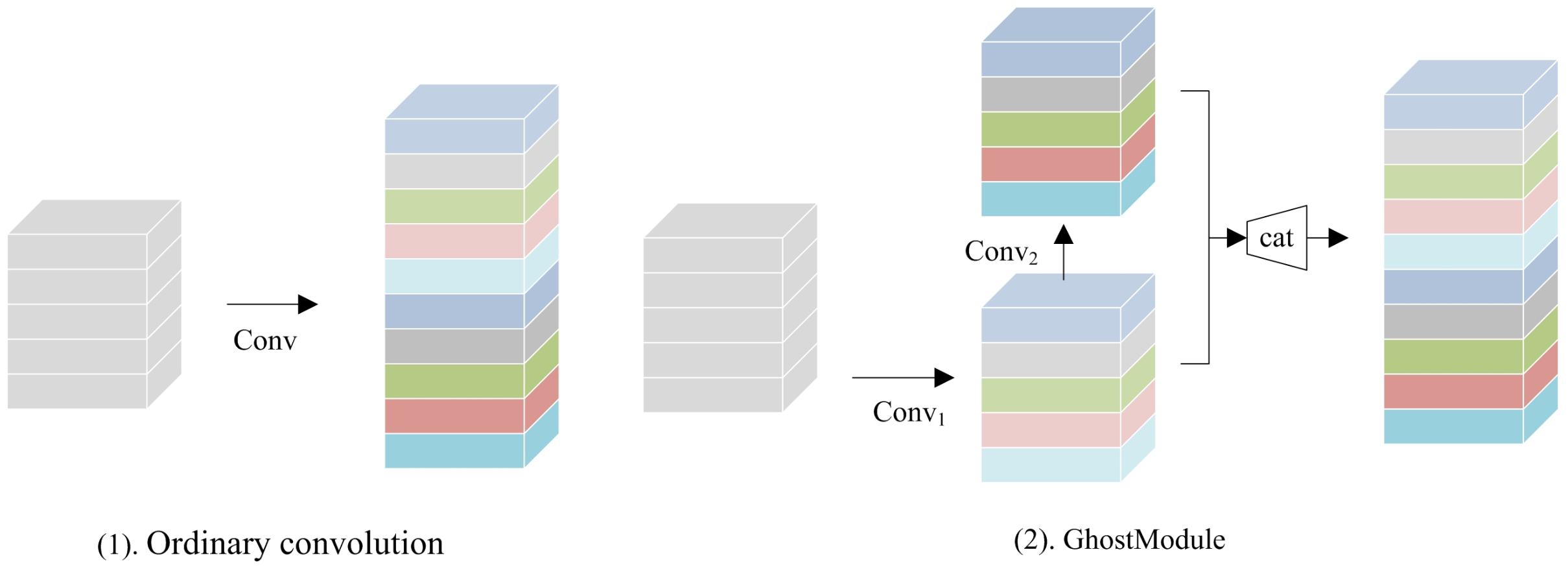
Through experiments, the Huawei team proved that a well-trained deep neural network usually contains rich or even redundant feature maps, and these redundant feature maps can be generated using the convolution operation with less computational cost. Based on this idea, Huawei’s GhostNet proposed in 2020 generates more feature maps using less computational cost; its core module is GhostModule. To obtain feature maps of the same dimension, for example, the ordinary convolution process and GhostModule in GhostNet are shown in Figure 1.

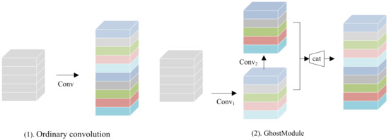
Figure 1. Ordinary convolution (1) and GhostModule (2).

In the ordinary convolution layer, there is the convolution process of the following Equation (1).

$$y=Conv\left(x\right).$$

(1)

In GhostModule, the convolution process is as shown in Equation (2).

$$y=Cat(Con{v}_1\left(x\right),Con{v}_2\left(Con{v}_1\left(x\right)\right)).$$

(2)

In the above equations [25], $xϵR^{C_{in}\times H_{in}\times W_{in}}$, $yϵR^{C_{out}\times H_{out}\times W_{out}}$, the $Conv$ in Equation (1) represents the ordinary convolution, that is, the filter number is the number of output channels $C_{out}$; each filter contains a number of kernels equal to the number of input channels $C_{in}$. In Equation (2), $Con{v}_1$ represents the normal convolution; the number of filters is $C_{out1}$. $Con{v}_2$ represents a cheaper convolution with fewer parameters; the number of filters is $C_{out2}$ and $C_{out2}=C_{out}-C_{out1}$.

3.2. Non-Local Neural Networks

In the convolution operation, the perceptual field size of the convolution is the convolution kernel size, which is generally selected as 3 × 3, 5 × 5, considering only the local area, making it a local operation. The fully connected neural network is a non-local global operation, but it introduces many parameters, which brings difficulties for optimization.

In the non-local neural networks proposed by Wang et al., the output of the designed non-local operation is the same size as the original image, and the calculation Equation (3) is as follows [30].

$$y_i=\frac{1}{C\left(x\right)}\sum _{\forall j}f(x_i,x_j)g\left(x_j\right).$$

(3)

x is the input feature, y is the output feature, and both are of the same dimension. $f(x_i,x_j)$ calculates the correlation between $x_i$ and $x_j$. When calculating the position correlation, the smaller $f(x_i,x_j)$ is, the more distant the two positions are, i.e., $x_j$ has a little influence on the position relationship of $x_i$. $g\left(x_j\right)$ is used to calculate the feature value of $x_i$ in $x_j$, and $C\left(x\right)$ is the normalization function to ensure that the overall information is unchanged before and after the transformation.

To simplifying the problem, consider g as the linear case, that is, $g\left(x_j\right)=W_g{x}_j$, where $W_g$ takes the 1 × 1 convolution of the spatial domain or the 1 × 1 × 1 convolution of the spatio-temporal domain. f can take a variety of different forms, including Gaussian, embedded Gaussian, etc., to calculate the correlation between the two points and finally, the overall Equation (4) of the nonlocal block is as follows [30]:

$$z_i=W_z{y}_i+x_i.$$

(4)

where $z_i$ is the final output with the same dimension as $x_i$. The nonlocal block can be implemented as a plug-and-play module for enhancing the extraction of global feature information.

4. Our Proposed Intelligent Weighted Object Detector

The task of object detection is to accomplish the identification and localization of objects in a specific scene. Generally, a simplified object detection process is shown in Figure 2 [43].

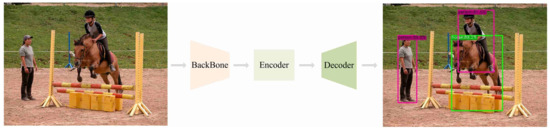
Figure 2. Object detection workflow diagram.

In Figure 2, there are three phases with different functions: BackBone, Encoder, and Decoder, where BackBone extracts features from the input image, Encoder fuses information from the feature map, and Decoder is responsible for decoding the fused features and outputting the category and localization information of the map. The improvements of YOLOX in this paper mainly focus on the BackBone and Encoder parts (YOLOXFPN). The specific improvements will be explained in detail in this section.

4.1. Overall Structure of the Model

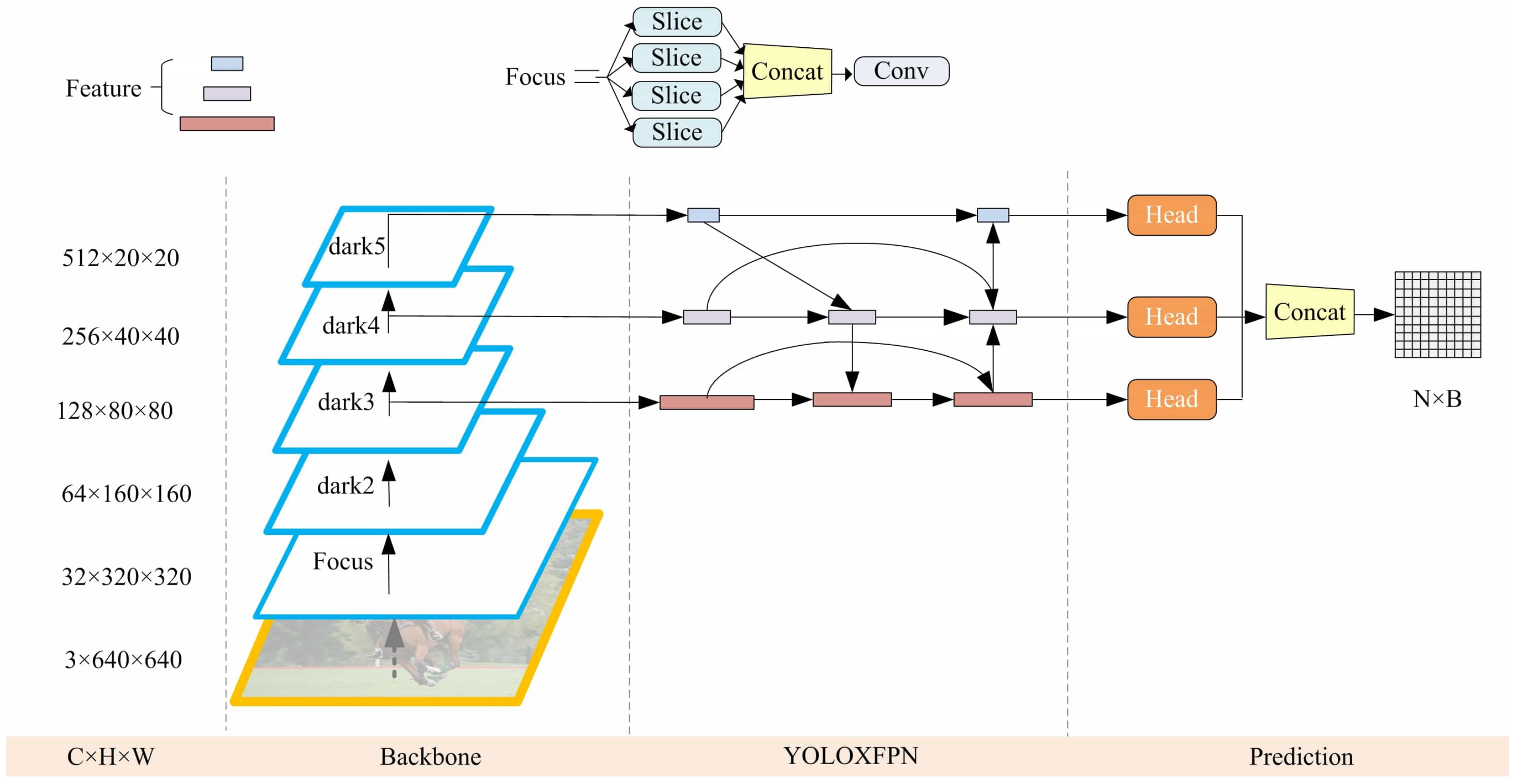
According to the depth, width, and backbone of the network, the advanced YOLOX model can be divided into seven models. The object detection model adopted in this paper is the YOLOX-S model, which follows the idea of label assignment and decoupling headers in YOLOX and adds a module for local image feature extraction and an extraction module for global features to the convolutional encoder. At the same time, the convolutional upscaling operation on the feature map is replaced with a less costly linear calculation, which reuses the feature maps in the network to avoid generating redundant features and adds weights to each layer in the final fusion to assist the network in learning to a better-weighted layer. The overall framework of the model is shown in Figure 3.

Figure 3. Overall framework diagram of our proposed intelligent weighted object detector, where $C\times H\times W$ are the number of channels, height, and width of the feature map, respectively. Focus, dark2, dark3, dark4, and dark5 denote the convolutional layers in the backbone network, Focus takes a value for every pixel in an image; the details of the structure of dark2, dark3, dark4 and dark5 are given in the following sections. The rectangular squares in YOLOXFPN are all output feature maps. In the prediction part, the head is the prediction head of the model, the structure is the same as in the YOLOX model, and the prediction result N × B is output after combining the results of all the detection heads, where N is the information of the prediction frame and B is the number of prediction frames.

4.2. Internal Structure of the Model

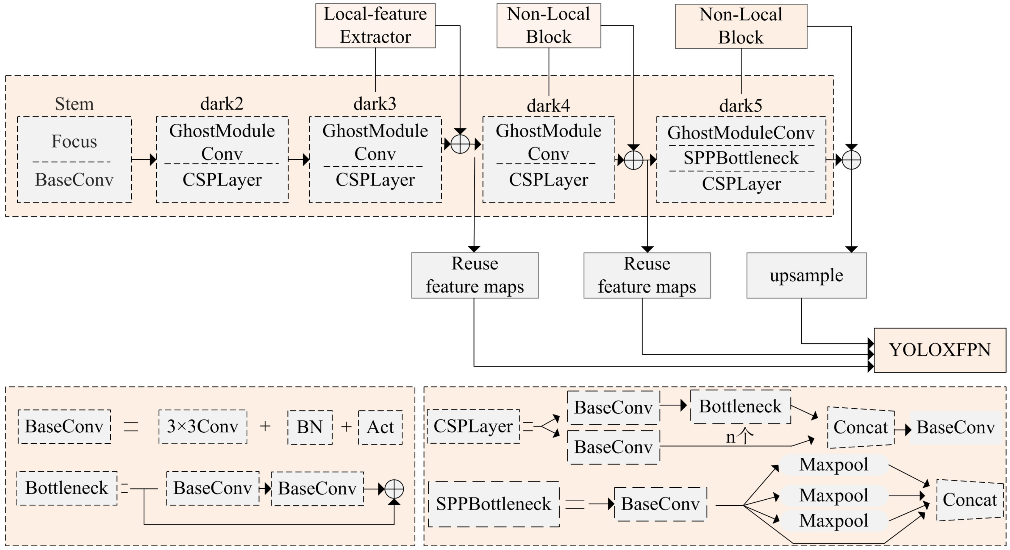
In the backbone network of the model, the shallow convolutional layer will obtain feature maps with richer detail information, so the feature extraction module of local images is placed in the lower layer so that the feature map of a single channel can receive more attention from the convolutional kernel. The deep feature map has rich semantic information, so the operation module of non-local operation is designed in the deep layer to enrich the semantic information of the feature map. Based on the backbone network of YOLOX-S, the internal structure of the improved YOLOX-S is shown in Figure 4.

Figure 4. Internal structure of our proposed intelligent weighted object detector.

• Local extraction feature module: local-feature extractor
  The local-feature extractor performs chunking and feature processing on the input feature maps; the specific structure is shown in Figure 5, where the 3 × 3 $DWConv$ is the deep convolution. The feature map of the lower layer is rich in detailed information, and considering that the feature map near the initial input end experiences fewer convolution layers, there will be too much noise, meaning that the detailed information of the deep feature map is lost, so the feature extraction module of the local image is added to the middle layer in the backbone network. In the local-feature extractor, the feature map $x_{in}ϵR^{C\times H\times W}$ is chopped to obtain four patches of the same size $x_iϵR^{C\times H/2\times W/2}$, where $i=1,2,3,4$, indicating four patches. After $x_i$ passes through the depthwise convolution, BN layer, and activation layer sequentially, it is returned to the size of $x_{in}$ according to the position of the original patch before chunking. In the local-feature extractor, the local image receives the attention of a single convolution, and the whole feature map no longer shares the same convolution kernel parameters, facilitating the extraction of detailed information in the image. This is be helpful for the detection of small objects;
  

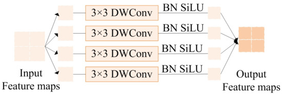  Figure 5. Local-feature extractor.
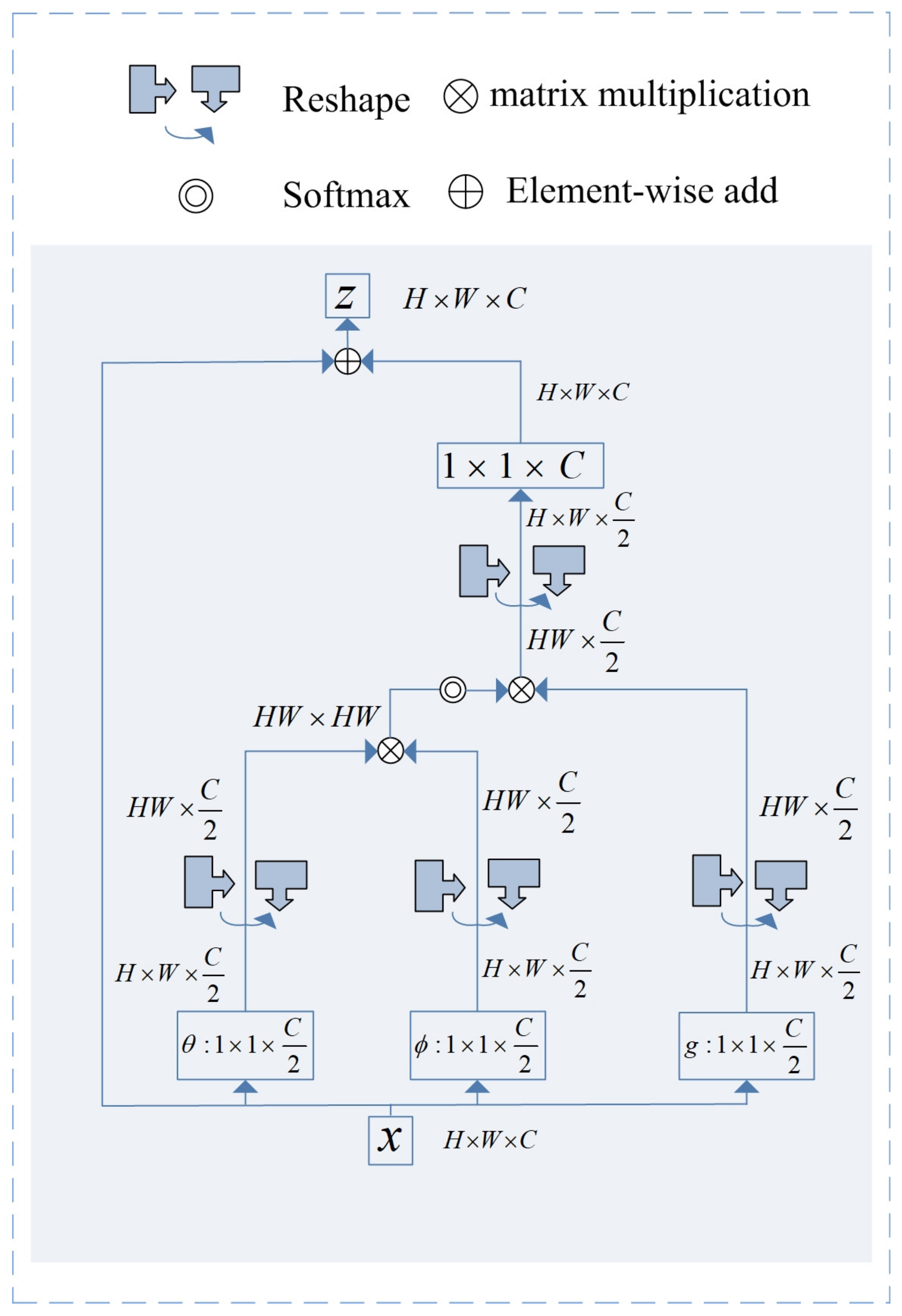
• Global feature extraction module: non-local block
  The specific structure of the non-local block is shown in Figure 6. In the non-local block, the input feature map first undergoes 1 × 1 convolution for channel adjustment and dimensional spreading; then, the correlation between any pixel point of the feature map and other pixel points is calculated. Finally, the features at each location are weighted using this correlation.
  

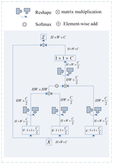  Figure 6. Non-local block.
  As shown in Figure 6, the exchange process in the global feature module is presented in Algorithm 1;
• GhostModuleConv
  In GhostModuleConv, the feature map $x_{in}ϵR^{C\times H\times W}$ passes through a filter of size 3 × 3, step size 2, and convolution number C to obtain $x_{dim1}ϵR^{C\times H/2\times W/2}$; then, $x_{dim1}$ is sent to depthwise convolution to obtain $x_{dim2}ϵR^{C\times H/2\times W/2}$ and the final $x_{out}ϵR^{2C\times H/2\times W/2}$ is obtained by concatenating the obtained $x_{dim1}$ and $x_{dim2}$;
• Reuse feature maps
  Inspired by GhostNet, which generates redundant feature maps when the feature maps go through multiple convolutional layers, and the fact that generating redundant maps causes the problem of computational redundancy, the idea of feature map reuse is proposed. The feature map reuse equation (5) is as follows.

  $$x_{out}=cat(x_{in1},x_{in2}).$$

  (5)

  where $x_{in2}$ is the feature map that has been generated in the network and has the same dimensions and size as the input feature map $x_{in1}$. When the number of channels of the output feature map is twice that of the input feature map, channel concatenation of the input feature map $x_{in1}$ with $x_{in2}$ can reduce the convolutional up-dimensioning operation for deeper feature maps with higher dimensionality. Thus, reusing feature maps can effectively avoid the dimensionality increase operation using 1 × 1 convolution and reduce a large number of convolution parameters.

  Algorithm 1 Transformation algorithm in the global feature extraction module

  Input: Feature map $xϵR^{batch\times H\times W\times C}$ Output: Global semantic information-rich feature maps $xϵR^{batch\times H\times W\times C}$

  1: According to $\theta \left(x_i\right)=W_{\theta }{x}_i$, $\varphi \left(x_j\right)=W_{\varphi }{x}_j$, use the embedding weights $W_{\theta }$ and $W_{\varphi }$ in $\theta \left(x_i\right)$ and $\varphi \left(x_j\right)$ to perform weight transformation on x to obtain $x_{\theta }ϵR^{batch\times H\times W\times C/2}$, $x_{\varphi }ϵR^{batch\times H\times W\times C/2}$, aiming to reduce the number of channels and computation. Use the linear embedding function $g\left(x_j\right)=W_g{x}_j$ for information exchange to obtain $x_gϵR^{batch\times H\times W\times C/2}$; 2: Reshape the output in Step 1 to obtain $x_{\theta }ϵR^{batch\times HW\times C/2}$, $x_{\varphi }ϵR^{batch\times HW\times C/2}$; 3: According to embedded Gaussian $f(x_i,x_j)=e^{{\theta \left(x_i\right)}^T\varphi \left(x_j\right)}$, after transposing $x_{\theta }$ in Step 2, the similarity is calculated by matrix multiplication with $x_{\varphi }$ to obtain $xϵR^{batch\times HW\times HW}$; 4: The output in Step 3 is softmax operated in the last dimension; then, perform the reshape operation with $x_g$ after matrix multiplication to obtain $xϵR^{batch\times H\times W\times C/2}$; 5: A convolutional kernel of size 1 × 1 and number C adjusts the output of Step 4 to the size of the channel when it enters the non-local block.

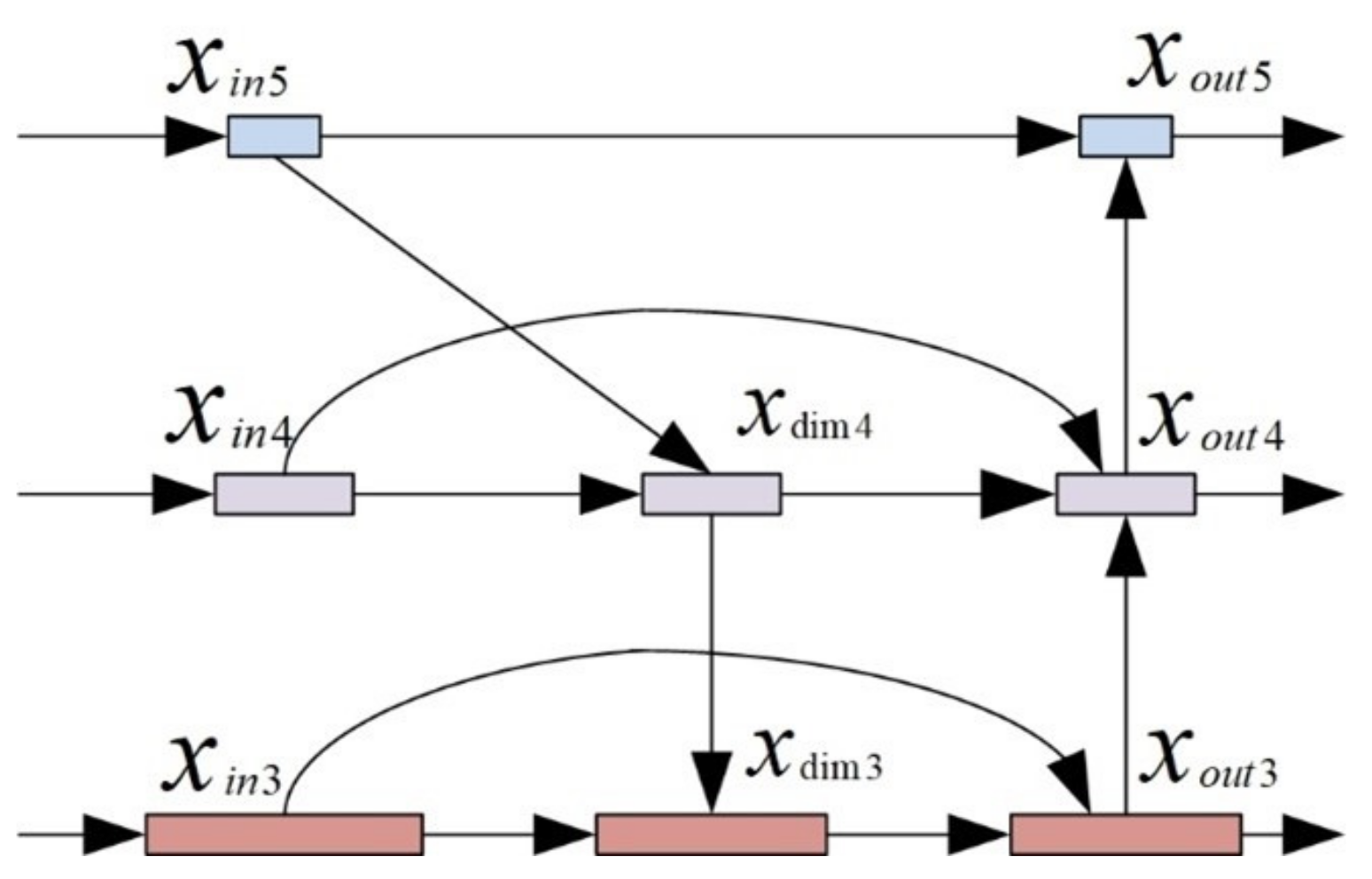
• YOLOXFPN
  The specific process of adding weights to the final output feature maps for dark3, dark4, and dark5 in YOLOXFPN is shown in Figure 7.
  

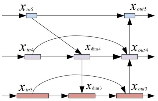  Figure 7. YOLOXFPN.
  Equation (6) for the output feature map with added weights is as follows [40]:

  $$\begin{array}{cc}\hfill & x_{out3}=Conv\left(\frac{w_{out3}^1\ast x_{in3}+w_{out3}^2\ast x_{dim3}}{w_{out3}^1+w_{out3}^2+\epsilon }\right),\hfill \\ \hfill & x_{out4}=Conv\left(\frac{w_{out4}^1\ast x_{in4}+w_{out4}^2\ast x_{dim4}+w_{out4}^3\ast Resize\left(x_{out3}\right)}{w_{out4}^1+w_{out4}^2+w_{out4}^3+\epsilon }\right),\hfill \\ \hfill & x_{out5}=Conv\left(\frac{w_{out5}^1\ast x_{in5}+w_{out5}^2\ast Resize\left(x_{out4}\right)}{w_{out5}^1+w_{out5}^2+\epsilon }\right).\hfill \end{array}$$

  (6)
  The calculation Equation (7) of the feature map generated in the middle is as follows [40]:

  $$\begin{array}{cc}\hfill & x_{dim4}=Conv\left(\frac{w_{dim4}^1\ast x_{in5}+w_{dim4}^2\ast Resize\left(x_{in4}\right)}{w_{dim4}^1+w_{dim4}^2+\epsilon }\right),\hfill \\ \hfill & x_{dim3}=Conv\left(\frac{w_{dim3}^1\ast Resize\left(x_{in3}\right)+w_{dim3}^2\ast x_{dim4}}{w_{dim3}^1+w_{dim3}^2+\epsilon }\right).\hfill \end{array}$$

  (7)
  To ensure that the divisor is not zero, $\epsilon =0.0001$. Before adding fusion, it is necessary to ensure that the fused feature maps have the same size. Therefore, is necessary to resize the feature maps, including adjusting the number of channels and the size of the feature maps.

5. Performance Analysis

5.1. Experimental Environment and Data Set

Table 1 shows the operating environment of the experiment.

Table 1. Experimental environment.

Category	Environmental Conditions
Operating System	CentOS 7.5
GPU	NVIDIA Tesla V100
Deep Learning Framework	PyTorch 1.7

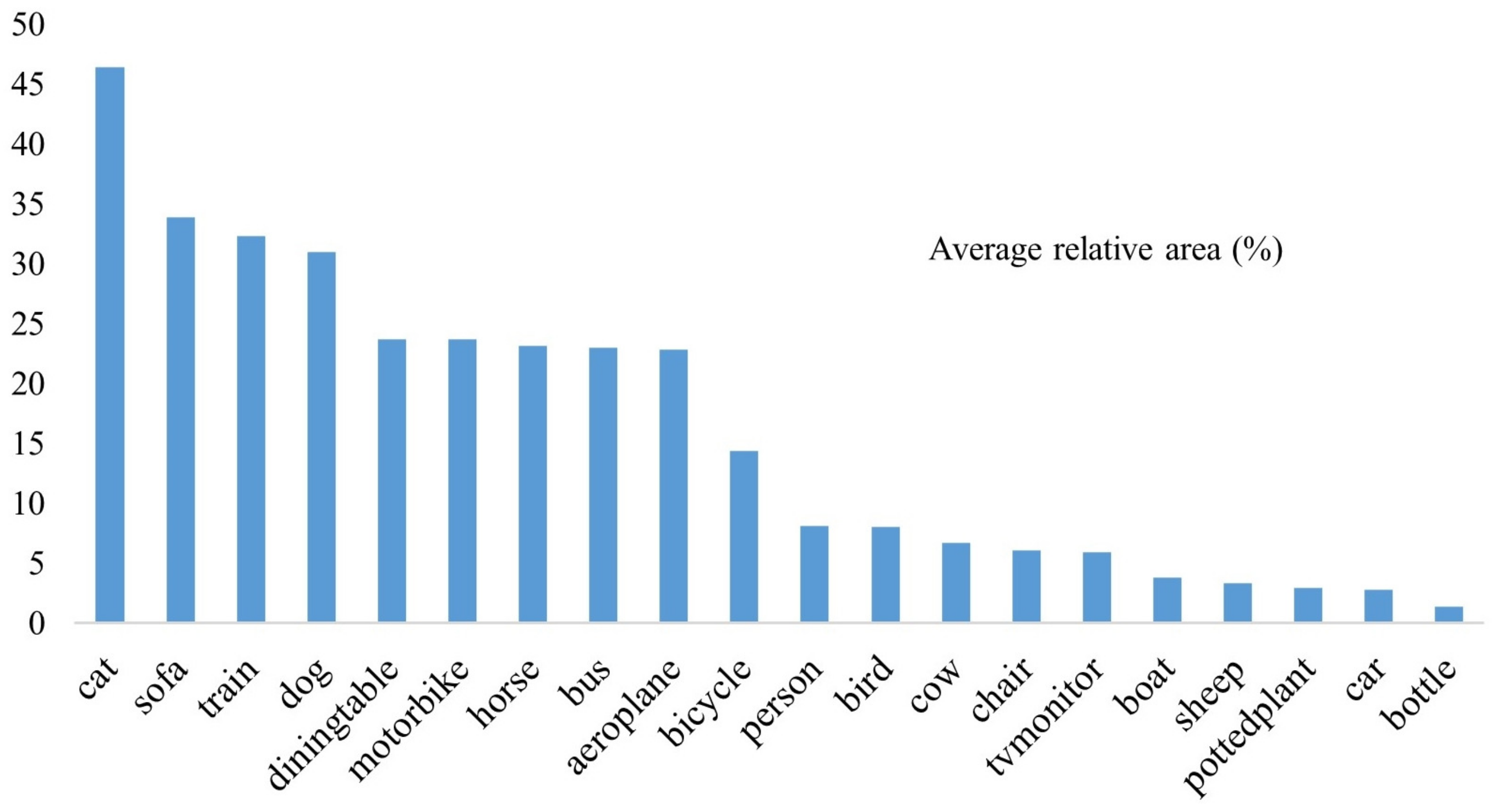
The experiments were conducted mainly on PASCAL VOC, a commonly used dataset for object detection. Combined, the PASCAL VOC 2007 and PASCAL VOC 2012 datasets have 16,551 images, of which the training and validation sets are allocated in at 9:1 ratio. The images in the test set are all from a total of 4952 images in PASCAL VOC 2007. The PASCAL VOC dataset contains 20 category labels: people, bird, cat, cow, dog, horse, sheep, airplane, bicycle, boat, bus, car, motorcycle, train, bottle, seat, dining table, potted plant, sofa, and TV. Referring to the percentage of each object category in the PASCAL VOC dataset in [44], the pixel percentage size of each category in the image is plotted as shown in Figure 8, where the average relative area is the median of the ratio of the area of the object’s bounding box to the area of the image.

Figure 8. Average relative area of object categories in the PASCAL VOC dataset.

By comparing the weight, size, and category accuracy of the YOLOX series models, the experiment selected the intermediate model YOLOX-S as the basis. Because the improved model structure did not conform to most of the pre-training model weights provided in baseline model YOLOX-S, the model was trained from scratch. After verifying the effectiveness of the improved model, comparative experiments were conducted on the same dataset with the well-established algorithm. In addition, the experiments were conducted on smaller-sized datasets in different scenarios, including the garbage dataset and the Steel Surface imperfections dataset, to verify the adaptability of the improved model to different situations. The TACO dataset is a growing spam dataset with woods, roads, and beaches as the shooting background, containing 1500 images, about 5000 annotations, and 60 categories. The Steel Surface NEU-CLS dataset was collected and published by Northeastern University. It includes 1800 images with six different categories of surface defects of hot-rolled steel strips, each of which contains 300 samples with the following defect categories: crazing, inclusion, patches, pitting surface, rolled in scale, and scratches. Similarly, the dataset assignment ratio is 9:1.

5.2. Experimental Evaluation Indicators

The experiment uses evaluation metrics commonly used in object detection [7].

• Average Precision: Abbreviated as AP, this is used to measure the detection effectiveness of the model on each object class and is calculated as follows:

  $$AP=\frac{1}{\sum r}\sum _{rϵ\{0,0.1,...,1\}}{\rho }_{interp\left(r\right)}{\rho }_{interp\left(r\right)}=\underset{\tilde{r}:\tilde{r}\ge r}{max}\rho \left(\tilde{r}\right).$$

  (8)
  Equation (8) represents the sum of the area enclosed between the PR curves and the horizontal coordinates of each category, where P is the accuracy of the object category $Precision$, and $Precision=TP/(TP+FP)$. R is the object category’s recall rate $Recall$, and $Recall=TP/(TP+FN)$, where $TP$ is the number of correctly predicted categories in a picture, $FP$ is the number of incorrectly predicted categories, and $FN$ is the number of categories not predicted. The average of the $AP$ values of each category obtained in Equation (8) is the final $mAP$. IOU (intersection over union) represents the ratio of intersection and merge between the prediction box and ground truth box, so $mA{P}_{50}$ represents the accuracy of the model when the IOU ratio threshold is 50;
• Frames per second: Abbreviated as FPS, this is used to measure the speed of model detection. The calculation in Equation (9) is shown below.

  $$\begin{array}{c}\hfill FPS=\frac{1}{Latency}.\end{array}$$

  (9)

  where $latency$ is the computation time of the model, i.e., the average time it takes for an image to be computed by the model;
• Model parameters and model computational complexity: This metric is found by inputting the same batch of images to the model and using the model weight calculation package profile in the Pytorch framework to calculate the parameter amount and calculation complexity of the model. The former unit is MB, and the larger the latter value, the more complex the model.

5.3. Experimental Results and Analysis

5.3.1. Ablation Experiments on the PASCAL VOC Dataset

In the experiments, considering that the reduction of the parameter amount in the backbone network affects the accuracy of the model, to verify the feasibility of cheap convolution, the feature map channel is boosted using cheap convolution in the YOLOX-S model and the feasibility of cheap convolution is verified by the accuracy comparison in Table 2. Meanwhile, to verify the feasibility of the local image feature extraction module, Table 2 also shows the variation of model accuracy, parameter size, and model computation on the validation set after adding the local feature extraction module. In addition, the size of the images in the ablation experiments were all 640 × 640.

Table 2. Comparison of model accuracy before and after adding GhostModuleConv.

Method	AP(%)	Parameters	GFLOPs
YOLOX-S [11]	76.75	9.0 M	26.8
+GhostModuleConv	77.88${}^{\uparrow 1.13}$	8.17 M	24.82
+Local-feature extractor	78.06${}^{\uparrow 1.13}$	8.17 M	24.83

In the encoder part of the model, as shown in Figure 4, the 3 × 3 convolution in the backbone network part in YOLOX-S is replaced with the cheap convolution GhostModuleConv in dark2, dark3, dark4, and dark5 for the upscaling operation on the feature maps. Take dark3 as an example where the input is $xϵR^{64\times 160\times 160}$, the output is $xϵR^{128\times 80\times 80}$; the filter taken in the YOLOX model has a convolution kernel of size 3 × 3, step size 2, and number 128; and the number of parameters needed is 64 × 128 × 3 × 3 = 73,728. After using GhostModuleConv, the number of parameters of convolution is (64 × 64 × 3 × 3) + (64 × 64 × 1 × 1) = 40,960; the parameters are reduced by nearly half. Table 2 shows that after replacing the convolution of raised channels used in the backbone network for feature extraction with a convolution method with fewer parameters, generating half of the desired input channels with 3 × 3 convolution, and generating the other half with depthwise convolution, there is no loss in the accuracy of the model based on a 0.83 M reduction in the convolution parameters but, on the contrary, the accuracy of the model is improved by 1.13%, while the complexity of the model is also reduced. The feasibility of using inexpensive convolution for feature extraction is verified. In the experiments, considering that the feature maps close to the input layer are noisy and significant detailed information of the feature maps in the deep layer is lost, the local-feature extractor module is added to dark3, as shown in Table 2. After adding the local-feature extractor module to the model, the accuracy of the model is further improved, and the feasibility of local image feature extraction after blocking the image is verified.

To verify the feasibility of the global feature extraction module non-local block, after using GhostModuleConv and the local-feature extractor in the backbone network, we add the non-local block to the model to verify the feasibility of the idea. If the non-local block is added to the lower network, it will introduce complicated computation due to the high resolution of the shallow feature map. On the contrary, if the non-local block is added to the deep network, it will not introduce too much computation and the deep feature map integrates the information of the lower feature map. Therefore, due to comprehensive consideration, the non-local block is added to layer 4 and layer 5 (dark4, dark5) of the backbone network in the experiment to enrich the global information of the deep feature maps. Table 3 shows the experimental results, where R.W represents the reuse and weighting operation of the feature maps, $A{P}_{@50:5:95}$ represents the result of averaging the values of IOU from 50% to 95% in 5% steps on the validation set, and $A{P}_{test}$ represents the effect of taking the values of IOU at 50% on the test set for each category of accuracy values.

Table 3. Comparison of model accuracy after adding the non-local block, reusing feature maps, and weighting feature maps.

Dark4	Dark5	Method	${\mathit{AP}}_{@50:5:95}$(%)	${\mathit{AP}}_{\mathit{test}}$(%)	Parameters
	✓	+Non-local block +R.W	77.86 77.98	- 82.5	8.75 M 8.49 M
✓		+Non-local block +R.W	78.35 78.33	- 82.6	8.44 M 7.70 M
✓	✓	+Non-local block +R.W	- 78.23	- 83.1	9.49 M 8.75 M

The idea of reusing the feature maps is to use the feature maps that have already been generated. Which layer to select the feature maps from and how to ensure that the existing information of the feature maps is not lost before using them are the key issues considered in the experiments. To follow the idea of not performing any convolution and pooling operations before reusing the feature map, the feature map that is generated should have the same number of channels as the feature map that needs to be raised. Considering that the feature map in the backbone network will have insufficient feature extraction when the feature map is not extracted by convolution in the deeper network, $x_{in2}$ in Equation (5) is adopted as $x_{in1}$, which means reusing its feature map. As seen from the data in Table 3, the accuracy of the model varies after adding the non-local block and R.W to different layers. After adding the non-local block to dark5, the accuracy of the model does not improve significantly, but it still performs better than the baseline model YOLOX-S; after adding R.W, the accuracy of the model improves, which verifies the effectiveness of reusing and weighting the feature maps. After adding the non-local b+9lock to dark4, the accuracy of the model improves significantly, which also confirms that the global information of the deep feature maps is the most abundant. Finally, after adding the non-local block to both dark4 and dark5 in the model and taking the feature map reuse and weighting operation for the feature map, the accuracy of the model is the best in the test set. The comprehensive experimental data verifies the feasibility of the idea.

5.3.2. Comparative Experiments on the PASCAL VOC Dataset

The experiment compares YOLOX-S, YOLOX-S${}^1$, and YOLOX-X${}^2$. YOLOX-S model is the baseline model and YOLOX-S${}^1$ is the model after improving it with the ideas proposed in this paper, using YOLOX-S as the base model. Meanwhile, in order to further verify the feasibility of reusing the feature maps, the difference between YOLOX-S${}^2$ and YOLOX-S${}^1$ is that before the final fusion, YOLOX-S${}^2$ takes a 1 × 1 convolution to adjust the number of channels of convolution and YOLOX-S${}^1$ takes the method in Equation (5) to adjust the number of channels. The accuracy values of each model in the experiments for each category in the PASCAL VOC 2007 test dataset are given in Table 4.

Table 4. Precision values for all classes on the PASCAL VOC 2007 test set for each model.

VOC 2007 Test	YOLOX-S	YOLOX-S${}^1$	YOLOX-S${}^2$
aeroplane	89.2	89.7	89.5
bicycle	89.1	89.8	88.5
bird	79.0	82.3	82.1
boat	75.9	77.7	77.4
bottle	73.0	73.5	72.2
bus	87.3	87.8	86.6
car	89.5	89.5	89.7
cat	86.6	87.3	87.9
chair	67.1	67.9	69.8
cow	87.0	88.9	87.5
diningtable	78.9	79.2	80.6
dog	84.9	86.1	85.2
horse	88.3	90.0	89.2
motorbike	88.0	89.0	87.8
person	86.6	86.7	86.8
pottedplant	62.0	61.1	61.6
sheep	81.9	85.1	85.3
sofa	78.4	79.6	79.7
train	84.7	86.3	86.9
tvmonitor	81.4	83.7	83.4

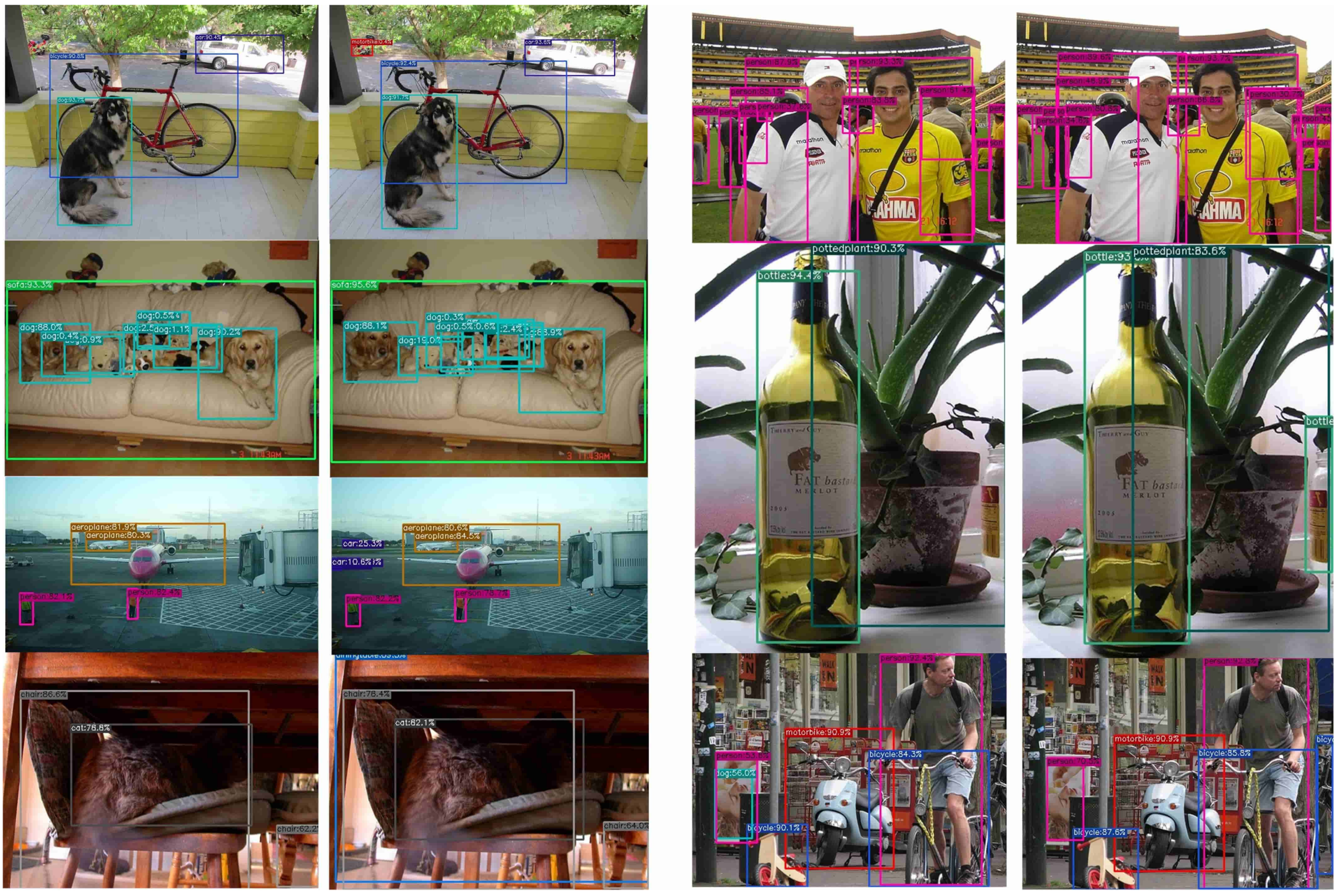
Analyzing Table 4, compared with Baseline YOLOX-S, the accuracy values of model YOLOX-S${}^2$ in all categories have different degrees of improvement. As can be seen from Figure 8, the pixel sizes of boat, sheep, potted plant, car, and bottle in the images are smaller compared to other categories, and the average relative area does not exceed 5%, while the accuracy of the categories is better on YOLO-S${}^1$, except for the category potted plant, which has slightly lower accuracy. In summary, the effectiveness of the feature extraction method for local images is verified; i.e., after the chopping operation of the feature map, the same feature map no longer shares the same convolutional kernel, but uses more convolutional kernels to do feature extraction for different parts of the same feature map, so that each small piece of the divided feature map can obtain the focus of independent convolution, thereby facilitating the network to extract more detailed information and improving the detection performance of the object. Analyzing the data in Table 4, the detection accuracy of all three models for the category potted plant is not high. From the images in the dataset, it can be observed that the category potted plant has more shapes; meanwhile, the number of the related image is low, and this affects the detection performance of the model. In the future, how to handle and detect categories of objects with variable and irregular shapes will also be a significant focus of research. Combining the data in Figure 8 and Table 4, among the classes with an average relative area between 5% and 10%, the categories person, bird, cow, chair, and tv monitor all have considerable point increases, notably, 3.3% for the category bird and 2.3% for tv monitor, further verifying the effectiveness of the algorithm in this paper. Comparing YOLOX-S${}^1$ and YOLOX-S${}^2$, the category detection results do not differ much and the performance of each object category accuracy is better in YOLOX-S${}^1$, thus proving that when fusing the network of the output layer, the output feature map does not need to use more convolutional kernels for feature extraction because it has already experienced many layers of convolutional layers. If using 1 × 1 convolution for channel dimensionality to achieve dimensionally consistent fusion prerequisites, more parameters will be produced, and reusing the already generated feature maps reduces the use of convolutional parameters. Comparing the results of YOLOX-S${}^1$ and YOLOX-S${}^2$, the feasibility of feature reuse in YOLOX-S${}^1$ is further proven, which also conforms to the verification in GhostNet; as the network becomes deeper, it generates more redundant feature maps that can be reused. In addition to the smaller percentage of categories that have improved in accuracy, others have also increased in points. Figure 9 shows the visualization results of YOLOX-S and YOLOX-S${}^1$. It can be seen that there are false detections, missed detections, and inaccurate localizations in YOLOX-S. Therefore, the visualization results further indicate that YOLOX-S${}^1$ performs better.

Figure 9. Visualization results of YOLOX-S and YOLOX-S${}^1$. Of the two sets of identical images, the left image is the detection output image of YOLOX-S and the right image is the detection output image of YOLOX-S${}^1$.

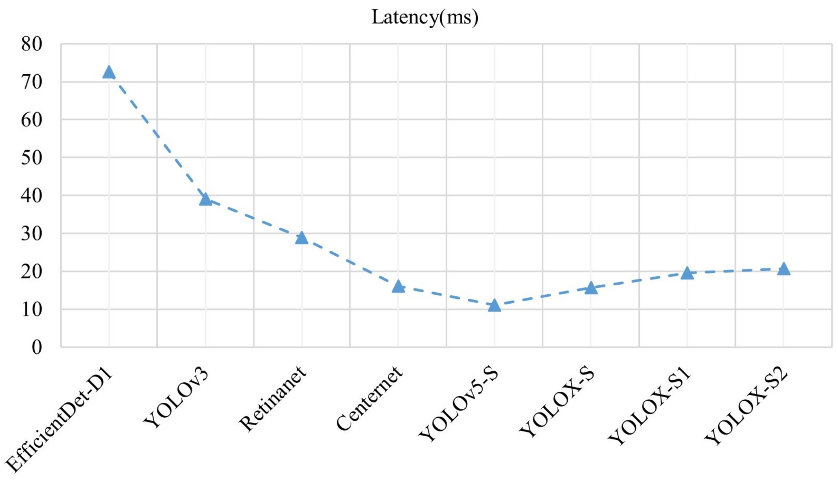
In recent years, many excellent models have emerged in the field of object detection. To verify the advantages of the algorithm in this paper, Table 5 shows the comparison between this algorithm and the advanced algorithm with the same metrics. The experiments were performed on the same data set with the same batch size (batch size = 1) and the same test environment. Figure 10 shows the inference time of each model in the same environment for the comparison, including the forward inference time of the model and excluding the NMS (1 ms/img) processing time of the model.

Table 5. Experimental results of each algorithm on the PASCAL VOC 2007 test dataset.

Model	Backbone	Size	Params. (M)	FPS	mAP${}_{50}$	mAP${}_{@50:5:95}$
EfficientDet-D1 [40]	Efficient-B1	640	6.56	13	72.7	51.3
YOLOv3 [45]	Efficient-B1	416	41.1	25	78.0	44.5
Retinanet [46]	ResNet50	600	37.97	34	78.9	51.5
Centernet [47]	ResNet50	512	32.67	62	76.5	48.7
YOLOv5-S [13]	CSPDarknet53	640	7.3	90	80.9	57.7
YOLOX-S [11]	CSPDarknet53	640	9.0	63	81.9	60.4
YOLOX-S${}^1$	Improved CSPDarknet53	640	8.75	51	83.1	61.6
YOLOX-S${}^2$	Improved CSPDarknet53	640	8.92	48	82.9	61.6

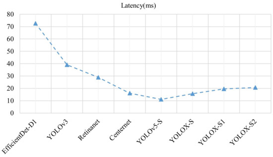
Figure 10. Speed comparison of each algorithm on the PASCAL VOC 2007 test dataset.

The sizes of the images in the experiments are all the image sizes used in training. Because there are seven models proposed in EfficientDet, the input image size of each model is not consistent, and the weight size of the models also varies greatly, the EfficientDet-D1 model with Efficient-B1 as the backbone network was selected to achieve fairness in comparison experiments. The backbone network darknet53 in the YOLOv3 model has been improved and has better performance in YOLOv4, so the original Darknet53 network in YOLOv3 is replaced with the Efficient-B1 network. ResNet is the most commonly used backbone network; the deeper the ResNet, the better the performance of the network will be, but this is also an exchange made at the expense of the weight size of the model as well as the detection speed. Selecting networks with lower networks, such as ResNet18 and ResNet34, results in poor model performance, so the intermediate network ResNet50 was selected as the backbone network for both the model Retinanet and Centernet. The detection performance of YOLOv5 is excellent and no changes are made in this paper. Similarly, to achieve fairness in comparison experiments, the YOLOv5-S model proposed in YOLOv5 is selected for comparison experiments. Observing the data in Table 5, the model YOLOv5-S performs optimally in terms of model size and detection speed, but its detection accuracy is inferior to that of YOLOX-S${}^1$ proposed in this paper. Analysis of the data shows that after improving on the baseline YOLOX-S model, the detection accuracy of the model is improved by 2.2% compared to YOLOv5-S, which further verifies the feasibility of the proposed improvement idea. According to the baseline model YOLOX-S and the improved YOLOX-S${}^1$ model, although the detection speed is slightly reduced, the weight size of the model is reduced compared with the original model and the detection accuracy is improved by one percentage point. Combined with the data in Table 4, the improved algorithm in this paper has more advantages in the object category with a smaller pixel share. Although the difference between YOLOX-S${}^1$ and YOLOX-S${}^2$ is not significant in each index, the comprehensive comparison shows that YOLOX-S${}^1$ performs better, thus proving the effectiveness of the idea of feature map reuse proposed in this paper from the aspect. The detection speed of the Centernet model is faster, but its weight size is too large to meet the storage requirements of mobile devices, and it is more limited in usage requirements for migration to embedded devices. Combining the data in the table and observing the line graph in Figure 7 shows that the improved YOLOX-S${}^1$ model does not have a substantial change in model speed compared to the original model, and the detection accuracy of the YOLOX-S${}^1$ model is higher.

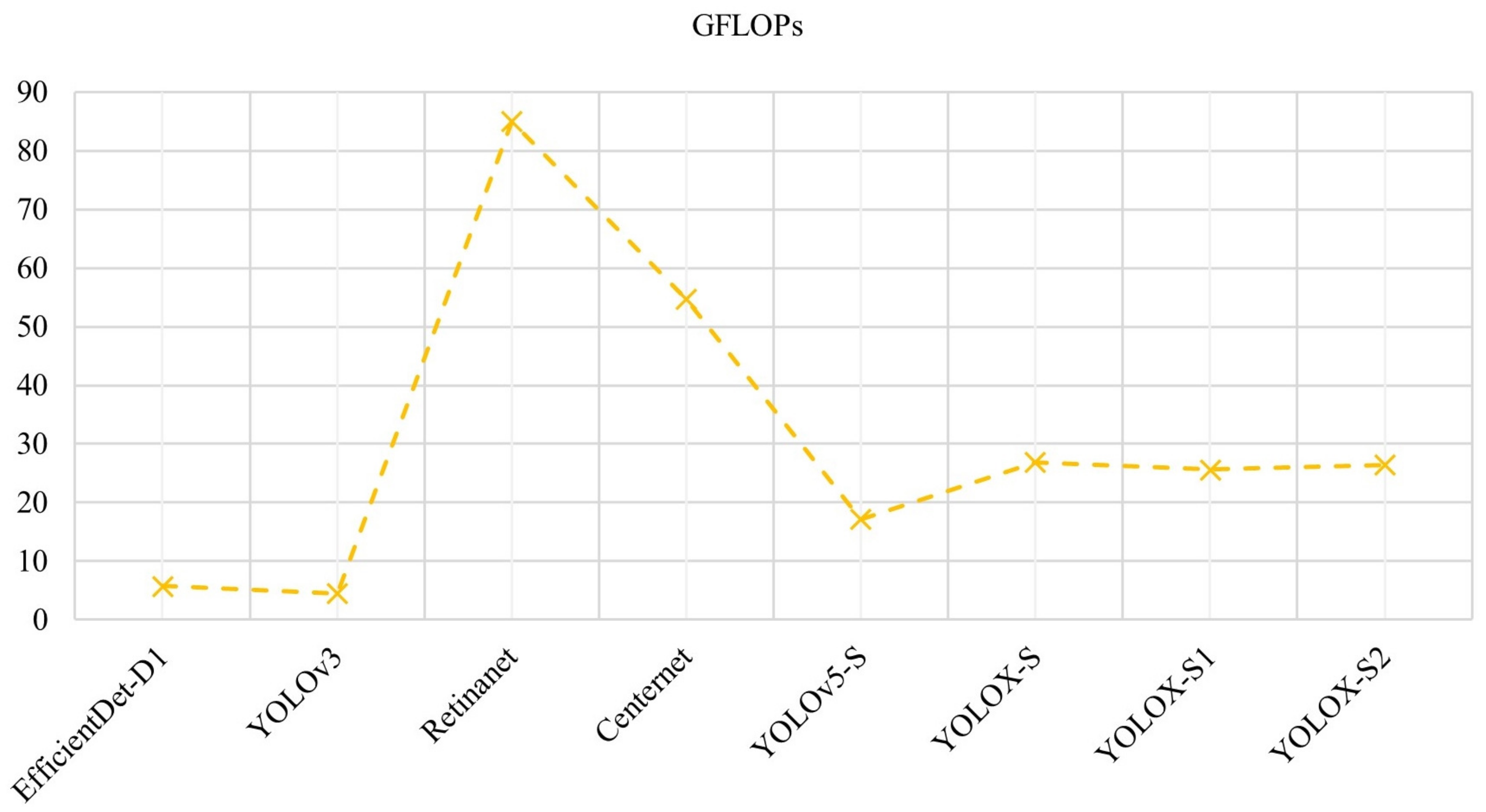
The number of floating-point operations (FLOPs) can be used to measure the computational complexity of the model. Since the computation of FLOPs is related to the input image size, the same image size is taken for each model in the experiments to compare the complexity of the model. Figure 11 shows the computational complexity of the model at an image size of 640 × 640.

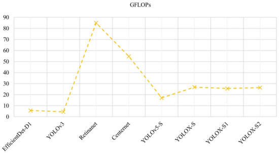
Figure 11. Computational complexity of the model.

As shown in Figure 11, the computational complexity of YOLOX-S${}^1$ remains equal to the original model, and although the model with lower model complexity is simpler, the accuracy of detection is lower. Combining the above experimental results, it is proven that after the improvement based on the original model YOLOX-S, YOLOX-S${}^1$ improves the accuracy of the model without adding any model weights or increasing the model complexity, so the YOLOX-S${}^1$ model proposed in this paper is more effective than the existing advanced models.

5.3.3. Experimental Results on TACO Dataset and NEU-CLS Dataset

In order to verify the generalization ability of the improved model YOLOX-S${}^1$, the base model YOLOX-S and the model YOLOX-S${}^1$ were trained on datasets in two different scenarios. Table 6 and Table 7 respectively show the experimental results of the two models on different data sets. Considering the uneven distribution of objects in the TACO dataset, only the garbage objects with a sample size greater than 200 are selected for the experiments. In the experiment, considering the problem of uneven object distribution in the TACO dataset, only garbage objects with a sample number of more than 200 were selected for the experiment, with a total of eight categories and 1086 images, including clear plastic bottle, plastic bottle cap, drink can, other plastic, plastic film, other plastic wrapper, unlabeled litter, and cigarette. The TACO dataset was divided into a training set and a verification set at a 9:1 ratio with no test set, and the experimental image size was 640 × 640. The NEU-CLS dataset was divided into a training set and a test set according to a 9:1 ratio; the separated training set was divided at a 9:1 ratio into a training set and a validation set, and the experimental image size was 320 × 320.

Table 6. Model detection results on the TACO dataset.

TACO	YOLOX-S	YOLOX-S${}^1$
clear plastic bottle	77.0	87.0
plastic bottle cap	60.4	72.0
drink can	75.9	79.6
other plastic	34.0	35.4
plastic film	46.3	55.1
other plastic wrapper	62.6	63.9
unlabeled litter	16.7	20.2
cigarette	15.4	26.4
$mA{P}_{50}$	48.5	54.9
$mA{P}_{@50:5:95}$	32.2	37.0

Table 7. Model detection results on the NEU-CLS dataset.

NEU-CLS	YOLOX-S	YOLOX-S${}^1$
crazing	34.4	40.0
inclusion	71.3	74.0
patches	82.7	89.4
pitted surface	58.9	64.0
rolled in scale	56.7	52.6
scratches	84.8	85.5
$mA{P}_{50}$	64.8	67.6
$mA{P}_{@50:5:95}$	31.1	33.6

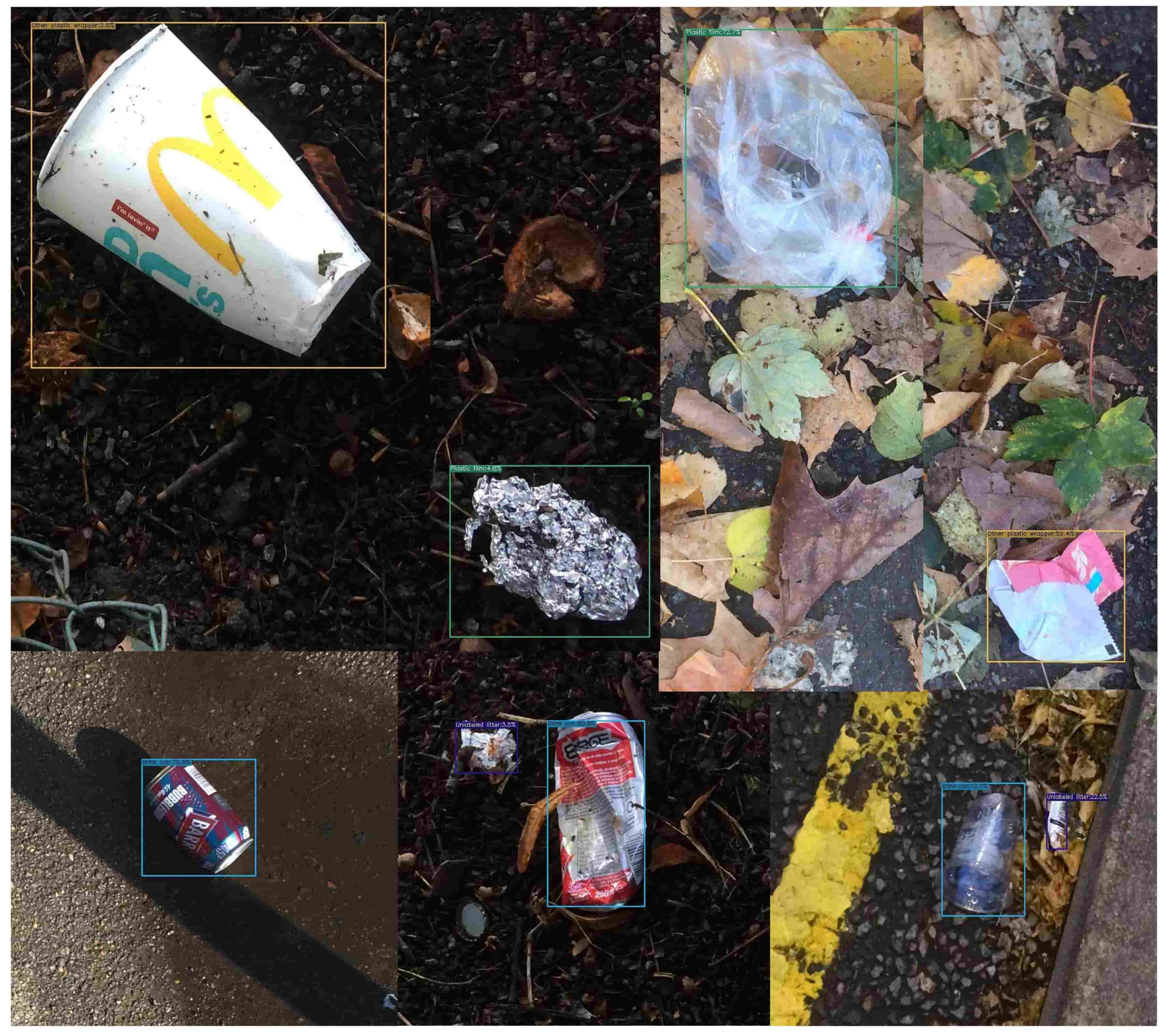
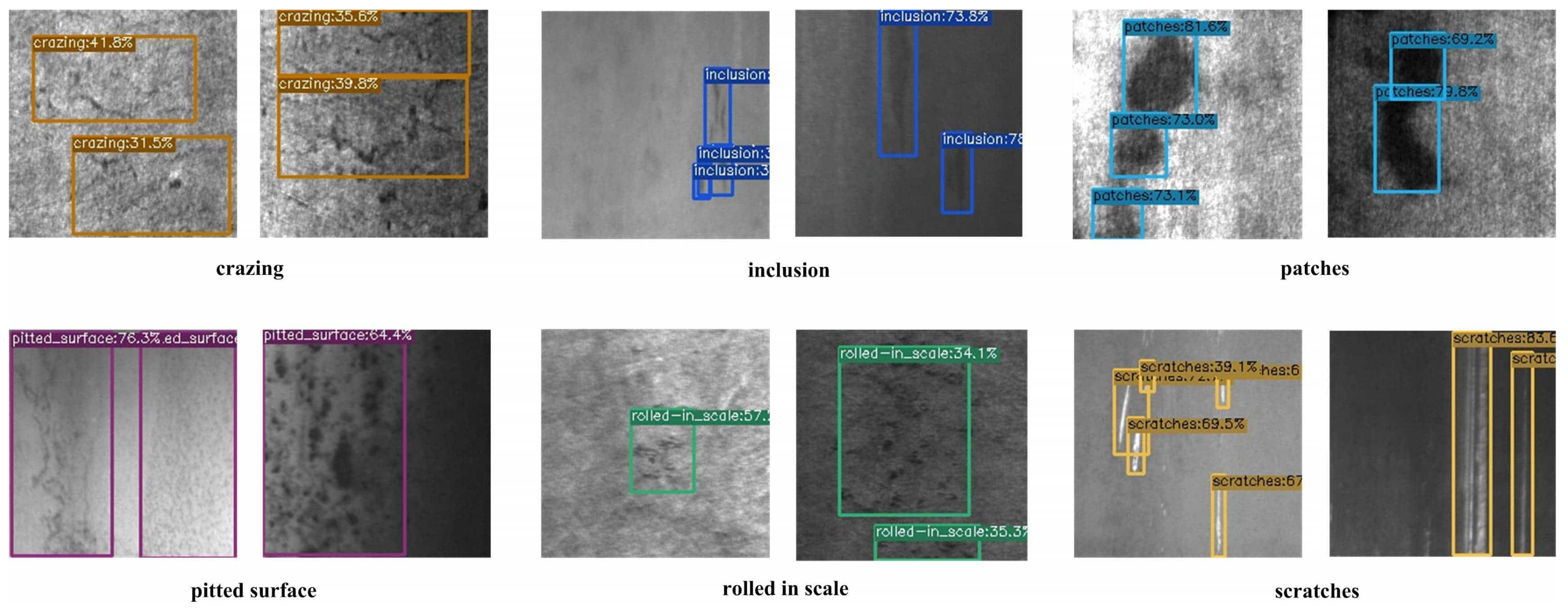
In the garbage dataset, due to the complex field environment and the irregular shapes and highly disturbed background interference of the object classes, while in the NEU-CLS dataset, the background is dim and category recognition is low, which leads to difficulties in the detection of the model. Combining the data in Table 6 and Table 7, it can be seen that YOLOX-S${}^1$ has the highest model detection accuracy both on the TACO dataset with stronger background interference and in the NEU-CLS dataset with grayscale images. Observing the category accuracies in Table 6, although the individual category results are not high, they all have accuracy improvements. For example, the accuracy of the categories unlabeled litter, and cigarette are improved by 3.5% and 11% in YOLOX-S${}^1$, respectively. In addition, in the final accuracy results, YOLOX-S${}^1$ improves by 6.4 percentage points over the baseline YOLOX-S, proving that YOLOX-S${}^1$ is more adaptable to more complex scenarios. Combined with the visualization in Figure 12, it can be seen that although the TACO dataset has a dark background and some object categories are not easily distinguished, YOLOX-S${}^1$ still performs well on the TACO dataset. Analyzing Table 7, YOLOX-S${}^1$ improved the average accuracy over YOLOX-S on the NEU-CLS dataset by 2.8%. Although YOLOX-S${}^1$ did not perform as well as YOLOX-S in the category rolled in scale, it performed better in the remaining five categories, especially in the categories crazing and pitted surface, where accuracy improved by 5.6% and 5.1%, respectively. In the future, the characteristics of rolled in scale will be deeply analyzed and YOLOX-S${}^1$ will be further studied to enrich the texture information of YOLOX-S${}^1$ and improve its accuracy when detecting similar rolled in scale categories. Figure 13 shows the detection effect of YOLOX-S${}^1$ for the same defect when the background dimness is inconsistent, further verifying that the improved YOLOX-S${}^1$ model is more adaptable to different scenes.

Figure 12. Visualization results of YOLOX-S${}^1$ on the TACO dataset.

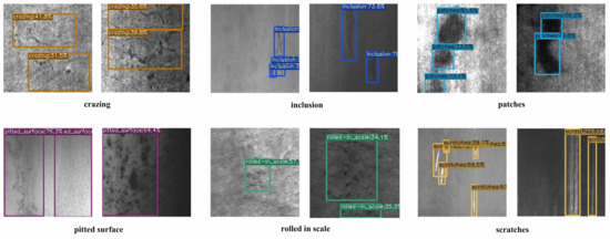
Figure 13. Visualization results of YOLOX-S${}^1$ on the NEU-CLS dataset.

5.4. Engineering Applications

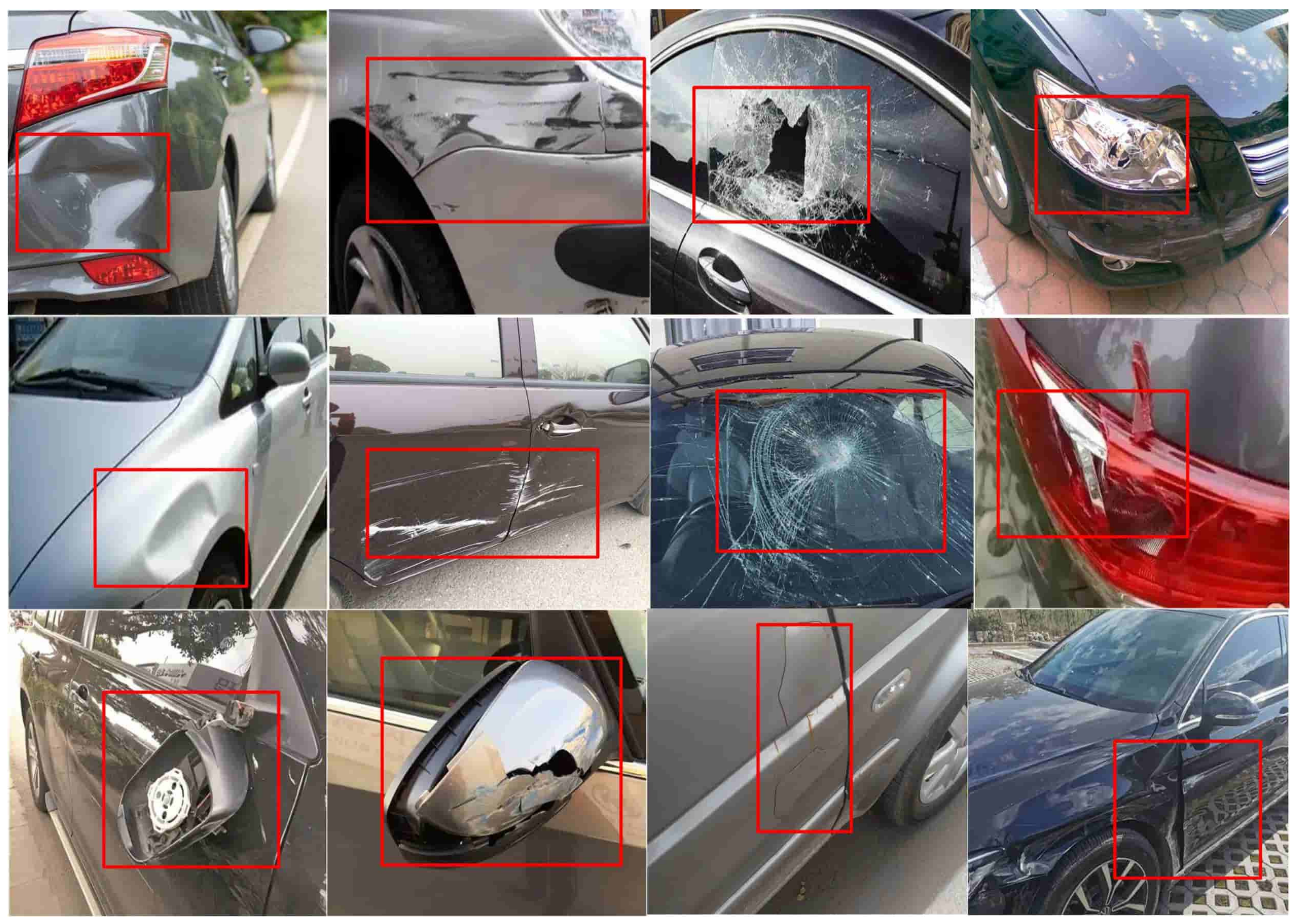
In the field of intelligent transportation, the detection and tracking of traffic violations is an important application scenario for object detection, that is, using object detection to find illegal motor vehicles in the motorway, vehicles privately occupying the emergency lane, toll station evasion phenomena, suspicious vehicles, and other traffic phenomena to assist public security and traffic control departments. Using the appearance of damaged suspicious vehicles for real-time detection will effectively improve the efficiency of public security while reducing the probability of security accidents. Figure 14 shows types of vehicle damage, including scratching, denting, cracking, creasing, piercing, broken lights, broken windows, and other damaging situations; the pictures are downloaded from the network.

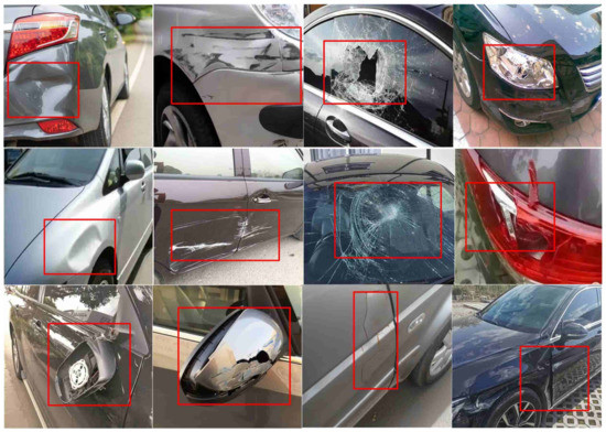
Figure 14. Vehicle exterior damage partial pictures.

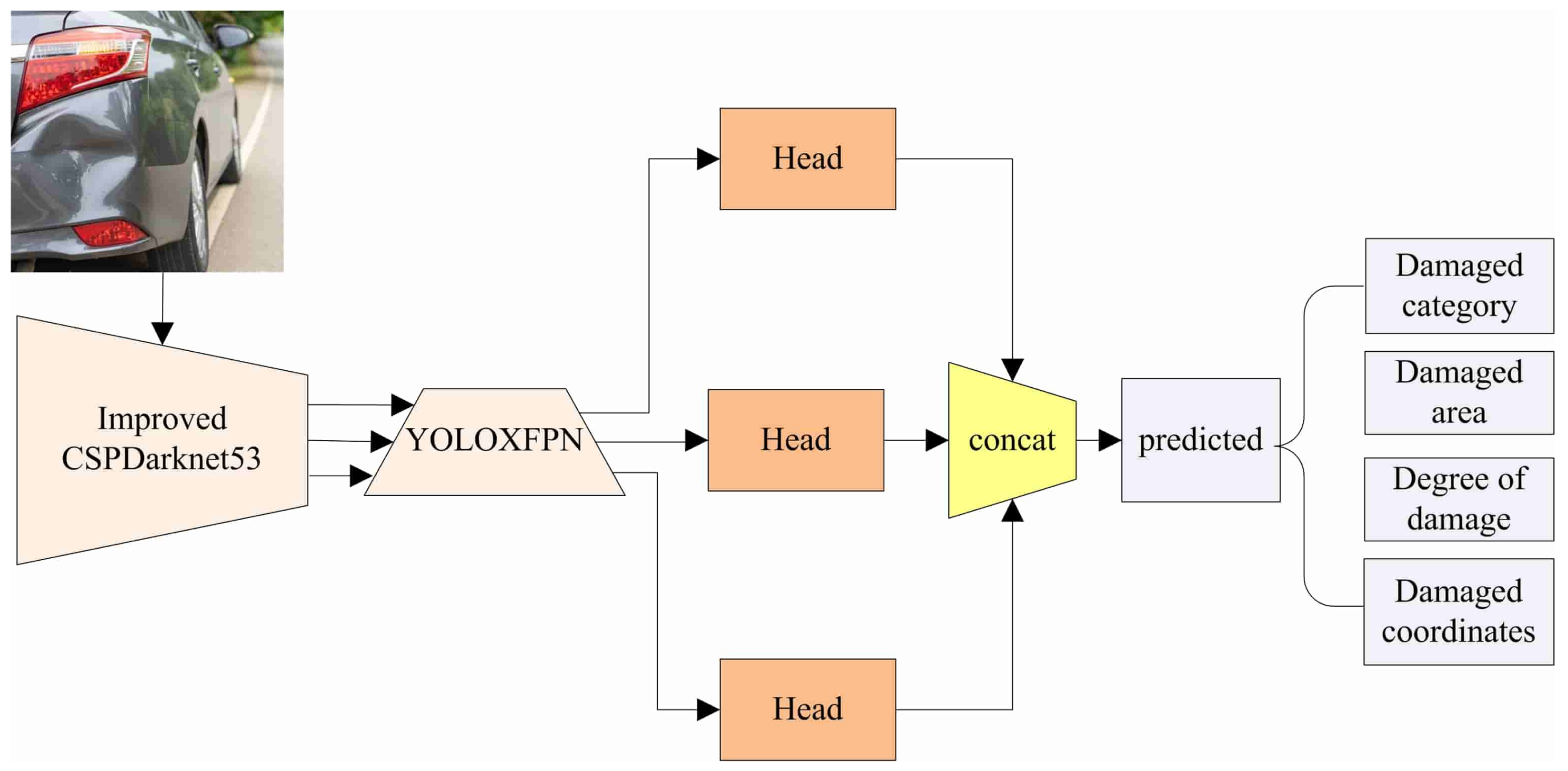
However, in practice, the same type of damage is complex and the damage range cannot be predicted in advance, so it is not realistic to use an anchor-based target detector for detection; therefore, as shown in Figure 15, localized damaged vehicle images are collected and used as the training set, and the model in this paper is used for training to pre-determine the vehicle damage category, in addition to predicting the damaged bounding box coordinates and the location of the damaged parts in the body of the output (front, rear, left, right). It then sets the damage threshold according to the degree of vehicle dent, scratch range, broken area and other preliminary judgment of the degree of damage, while according to the set threshold, the degree of damage is classified as light damage, moderate damage, or heavy damage. In addition, the positioned damage area map is saved.

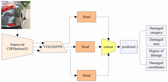
Figure 15. Damaged area inspection process.

In practice, the damage to vehicle parts is complex and varied, and there is a “coexistence” situation, i.e., the same area can be scratched and dented, which makes detection difficult. This problem is similar to object overlap in the object detection. Therefore, in the future, methods to solve object overlap can be investigated to improve the detection accuracy of this model in scenes with complex shapes and overlapping objects.

6. Conclusions and Future Work

In this paper, we take YOLOX-S as the baseline model, add a local image feature extraction operation to chunk the feature map to increase the detailed information of features, and introduce a global feature extraction module to calculate the correlation of feature points to enrich the semantic information of the feature map. To make the model focus on the feature layers that contribute more to the final detection result, we add weights to the feature layers involved in prediction. In addition, this paper also introduces an inexpensive convolution operation to reduce the convolution parameters in the backbone network and proposes the idea that feature maps can be reused. Experimental results show the effectiveness of the above improvements, which achieve improvement of the detection accuracy of the model without increasing the model weights. Finally, according to analysis of the experimental data and concrete reflections on engineering applications, in the future work, we will focus on improving the detection accuracy of complex categories and design detection heads specifically for complex tasks, so that the model can adapt to scenes with overlapping and complex objects.

References

- Wang, X.; Li, Q.; Xiong, N.; Pan, Y. Ant Colony Optimization-Based Location-Aware Routing for Wireless Sensor Networks. Int. Conf. Wirel. Algorithms 2008, 5258, 109–120. [Google Scholar]
- Wan, R.; Xiong, N.; Loc, N. An energy-efficient sleep scheduling mechanism with similarity measure for wireless sensor networks. Hum.-Centric Comput. Inf. Sci. 2018, 8, 18. [Google Scholar] [CrossRef] [Green Version]
- Lu, Y.; Wu, S.; Fang, Z.; Xiong, N.; Yoon, S.; Park, D.S. Exploring finger vein based personal authentication for secure IoT. Future Gener. Comput. Syst. 2017, 77, 149–160. [Google Scholar] [CrossRef]
- Gao, K.; Han, F. Connected Vehicle as a Mobile Sensor for Real Time Queue Length at Signalized Intersections. Sensors 2019, 19, 2059. [Google Scholar] [CrossRef] [Green Version]
- Jiang, Y.; Tong, G.; Yin, H.; Xiong, N. A Pedestrian Detection Method Based on Genetic Algorithm for Optimize XGBoost Training Parameters. IEEE Access 2019, 7, 118310–118321. [Google Scholar] [CrossRef]
- Yan, L.; Sheng, M.; Wang, C.; Gao, R.; Yu, H. Hybrid neural networks based facial expression recognition for smart city. Multimed. Tools Appl. 2022, 81, 319–342. [Google Scholar] [CrossRef]
- Xiao, Y.; Tian, Z.; Yu, J.; Zhang, Y. A review of object detection based on deep learning. Multimed. Tools Appl. 2020, 79, 23729–23791. [Google Scholar] [CrossRef]
- Selukar, M.; Jain, P.; Kumar, T. A device for effective weed removal for smart agriculture using convolutional neural network. Int. J. Syst. Assur. Eng. Manag. 2022, 13, 397–404. [Google Scholar] [CrossRef]
- Zhang, H.; Wang, Y.; Dayoub, F.; Sünderhauf, N. VarifocalNet: An IoU-aware Dense Object Detector. In Proceedings of the 2021 IEEE/CVF Conference on Computer Vision and Pattern Recognition, Nashville, TN, USA, 20–25 June 2021; pp. 8510–8519. [Google Scholar]
- Zhou, X.; Koltun, V.; Krähenbühl, P. Probabilistic Two-Stage Detection. arXiv 2021, arXiv:2103.07461. [Google Scholar]
- Ge, Z.; Liu, S.; Wang, F.; Li, Z. YOLOX: Exceeding YOLO Series in 2021. arXiv 2021, arXiv:2107.08430. [Google Scholar]
- Zhu, X.; Su, W.; Lu, L.; Li, B. Deformable DETR: Deformable Transformers for End-to-End Object Detection. arXiv 2021, arXiv:2010.04159. [Google Scholar]
- Zhu, X.; Lyu, S.; Wang, X.; Zhao, Q. TPH-YOLOv5: Improved YOLOv5 Based on Transformer Prediction Head for Object Detection on Drone-captured Scenarios. In Proceedings of the 2021 IEEE/CVF International Conference on Computer Vision Workshops (ICCVW), Montreal, BC, Canada, 11–17 October 2021; pp. 2778–2788. [Google Scholar]
- Yang, Z.; Liu, S.; Hu, H.; Wang, L.; Lin, S. RepPoints: Point Set Representation for Object Detection. In Proceedings of the 2019 IEEE/CVF International Conference on Computer Vision, Seoul, Korea, 27 October–2 November 2019; pp. 9656–9665. [Google Scholar]
- Mittal, P.; Singh, R.; Sharma, A. Deep learning-based object detection in low-altitude UAV datasets: A survey. Image Vis. Comput. 2020, 104, 104046. [Google Scholar] [CrossRef]
- Yan, L.; Fu, J.; Wang, C.; Ye, Z.; Chen, H.; Ling, H. Enhanced network optimized generative adversarial network for image enhancement. Multimed. Tools Appl. 2021, 80, 14363–14381. [Google Scholar] [CrossRef]
- Huang, G.; Liu, S.; Van der Maaten, L.; Weinberger, K.Q. CondenseNet: An Efficient DenseNet Using Learned Group Convolutions. In Proceedings of the 2018 IEEE/CVF Conference on Computer Vision and Pattern Recognition, Salt Lake City, UT, USA, 18–23 June 2018; pp. 2752–2761. [Google Scholar]
- Sandler, M.; Howard, A.; Zhu, M.; Zhmoginov, A. MobileNetV2: Inverted Residuals and Linear Bottlenecks. In Proceedings of the 2018 IEEE/CVF Conference on Computer Vision and Pattern Recognition (CVPR), Salt Lake City, UT, USA, 18–23 June 2018; pp. 4510–4520. [Google Scholar]
- Howard, A.; Sandler, M.; Chen, B.; Wang, W. Searching for MobileNetV3. In Proceedings of the 2019 IEEE/CVF International Conference on Computer Vision (ICCV), Seoul, Korea, 27 October–2 November 2019; pp. 1314–1324. [Google Scholar]
- Zhang, X.; Zhou, X.; Lin, M.; Sun, J. ShuffleNet: An Extremely Efficient Convolutional Neural Network for Mobile Devices. In Proceedings of the 2018 IEEE/CVF Conference on Computer Vision and Pattern Recognition, Salt Lake City, UT, USA, 18–23 June 2018; pp. 6848–6856. [Google Scholar]
- Ma, N.; Zhang, X.; Zheng, H.; Sun, J. ShuffleNet V2: Practical Guidelines for Efficient CNN Architecture Design. In Proceedings of the European Conference on Computer Vision 2018, Munich, Germany, 9 October 2018; pp. 122–138. [Google Scholar]
- Tan, M.; Le, Q.V. EfficientNet: Rethinking Model Scaling for Convolutional Neural Networks. arXiv 2019, arXiv:1905.11946. [Google Scholar]
- Tan, M.; Le, Q.V. EfficientNetV2: Smaller Models and Faster Training. arXiv 2021, arXiv:2104.00298. [Google Scholar]
- Zhang, H.; Wu, C.; Zhang, Z. ResNeSt: Split-Attention Networks. arXiv 2020, arXiv:2004.08955. [Google Scholar]
- Han, K.; Wang, Y.; Tian, Q.; Guo, J. GhostNet: More Features From Cheap Operations. In Proceedings of the 2020 IEEE/CVF Conference on Computer Vision and Pattern Recognition (CVPR), Seattle, WA, USA, 13–19 June 2020; pp. 1577–1586. [Google Scholar]
- Yang, L.; Jiang, H.; Cai, R.; Wang, Y.; Song, S.; Huang, G.; Tian, Q. CondenseNet V2: Sparse Feature Reactivation for Deep Networks. In Proceedings of the 2021 IEEE/CVF Conference on Computer Vision and Pattern Recognition (CVPR), Nashville, TN, USA, 20–25 June 2021; pp. 3568–3577. [Google Scholar]
- Han, D.; Yun, S.; Heo, B.; Yoo, Y. Rethinking Channel Dimensions for Efficient Model Design. arXiv 2020, arXiv:2007.00992. [Google Scholar]
- Wang, G.; Yuan, Y.; Chen, X.; Li, J. Learning Discriminative Features with Multiple Granularities for Person Re-Identification. In Proceedings of the 26th ACM International Conference on Multimedia, New York, NY, USA, 15 October 2018; pp. 274–282. [Google Scholar]
- Hu, H.; Zhang, Z.; Xie, Z.; Lin, S. Local Relation Networks for Image Recognition. In Proceedings of the 2019 IEEE/CVF International Conference on Computer Vision (ICCV), Seoul, Korea, 27 October–2 November 2019; pp. 3463–3472. [Google Scholar]
- Wang, X.; Girshick, R.; Gupta, A.; He, K. Non-local Neural Networks. In Proceedings of the 2018 IEEE/CVF Conference on Computer Vision and Pattern Recognition, Salt Lake City, UT, USA, 18–23 June 2018; pp. 7794–7803. [Google Scholar]
- Carion, N.; Massa, F.; Synnaeve, G. End-to-End Object Detection with Transformers. arXiv 2020, arXiv:2005.12872. [Google Scholar]
- Chen, Y.; Dai, X.; Chen, D.; Liu, M.; Dong, X.; Yuan, L.; Liu, Z. Mobile-Former: Bridging MobileNet and Transformer. arXiv 2021, arXiv:2108.05895. [Google Scholar]
- Yang, Z.; Li, Z.; Jiang, X.; Gong, Y.; Yuan, Z.; Zhao, D.; Yuan, C. Focal and Global Knowledge Distillation for Detectors. arXiv 2022, arXiv:2111.11837. [Google Scholar]
- Sun, J.; Shen, Z.; Wang, Y.; Bao, H.; Zhou, X. LoFTR: Detector-Free Local Feature Matching with Transformers. arXiv 2021, arXiv:2104.00680. [Google Scholar]
- Sun, P.; Zhang, R.; Jiang, Y.; Kong, T.; Xu, C.; Zhan, W.; Tomizuka, M.; Li, L.; Yuan, Z.; Wang, C.; et al. Sparse R-CNN: End-to-End Object Detection with Learnable Proposals. In Proceedings of the 2021 IEEE/CVF Conference on Computer Vision and Pattern Recognition (CVPR), Nashville, TN, USA, 20–25 June 2021; pp. 14449–14458. [Google Scholar]
- Lin, T.-Y.; Dollár, P.; Girshick, R.; He, K. Feature Pyramid Networks for Object Detection. In Proceedings of the 2017 IEEE Conference on Computer Vision and Pattern Recognition, Honolulu, HI, USA, 21–26 July 2017; pp. 936–944. [Google Scholar]
- Liu, S.; Qi, L.; Qin, H.; Shi, J. Path Aggregation Network for Instance Segmentation. In Proceedings of the 2018 IEEE/CVF Conference on Computer Vision and Pattern Recognition (CVPR), Salt Lake City, UT, USA, 18–23 June 2018; pp. 8759–8768. [Google Scholar]
- Zhao, Q.; Sheng, T.; Wang, Y.; Tang, Z. M2Det: A Single-Shot Object Detector Based on Multi-Level Feature Pyramid Network. In Proceedings of the AAAI Conference on Artificial Intelligence, Honolulu, HI, USA, 27 January 2019; pp. 9259–9266. [Google Scholar]
- Liu, S.; Huang, D.; Wang, Y. Learning Spatial Fusion for Single-Shot Object Detection. arXiv 2019, arXiv:1911.09516. [Google Scholar]
- Tan, M.; Pang, R.; Le, Q.V. EfficientDet: Scalable and Efficient Object Detection. In Proceedings of the 2020 IEEE/CVF Conference on Computer Vision and Pattern Recognition (CVPR), Seattle, WA, USA, 13–19 June 2020; pp. 10778–10787. [Google Scholar]
- Guo, C.; Fan, B.; Zhang, Q.; Xiang, S.; Pan, C. AugFPN: Improving Multi-scale Feature Learning for Object Detection. In Proceedings of the 2020 IEEE/CVF Conference on Computer Vision and Pattern Recognition (CVPR), Seattle, WA, USA, 13–19 June 2020; pp. 2592–12601. [Google Scholar]
- Zhang, D.; Zhang, H.; Tang, J.; Wang, M.; Hua, X.; Sun, Q. Feature Pyramid Transformer. In Proceedings of the 16th European Conference on Computer Vision(ECCV), Glasgow, UK, 23–28 August 2020; pp. 323–339. [Google Scholar]
- Chen, Q.; Wang, Y.; Yang, T.; Zhang, X.; Cheng, J.; Sun, J. You Only Look One-level Feature. arXiv 2021, arXiv:2103.09460. [Google Scholar]
- Krishna, H.; Jawahar, C.V. Improving Small Object Detection. In Proceedings of the 2017 4th IAPR Asian Conference on Pattern Recognition (ACPR), Nanjing, China, 26–29 November 2017; pp. 340–345. [Google Scholar]
- Redmon, J.; Farhadi, A. YOLOv3: An Incremental Improvement. arXiv 2018, arXiv:1804.02767. [Google Scholar]
- Lin, T.-Y.; Goyal, P.; Girshick, R.; He, K.; Dollár, P. Focal Loss for Dense Object Detection. In Proceedings of the 2017 IEEE International Conference on Computer Vision (ICCV), Venice, Italy, 22–29 October 2017; pp. 2999–3007. [Google Scholar]
- Zhou, X.; Wang, D.; Krähenbühl, P. Objects as Points. arXiv 2019, arXiv:1904.07850. [Google Scholar]
Publisher’s Note: MDPI stays neutral with regard to jurisdictional claims in published maps and institutional affiliations. |
© 2022 by the authors. Licensee MDPI, Basel, Switzerland. This article is an open access article distributed under the terms and conditions of the Creative Commons Attribution (CC BY) license (https://creativecommons.org/licenses/by/4.0/).