Abstract
By solving a Marchenko equation, Green’s functions at an arbitrary (inner) depth level inside an unknown elastic layered medium can be retrieved from single-sided reflection data, which are collected at the top of the medium. To date, it has only been possible to obtain an exact solution if the medium obeyed stringent monotonicity conditions and if all forward-scattered (non-converted and converted) transmissions between the acquisition level and the inner depth level were known a priori. We introduce an alternative Marchenko equation by revising the window operators that are applied in its derivation. We also introduce an auxiliary equation for transmission data, which are collected at the bottom of the medium, and a coupled equation, which is based on both reflection and transmission data. We show that the joint system of the Marchenko equation, the auxiliary equation and the coupled equation can be succesfully inverted when broadband reflection and transmission data are available. This results in a novel methodology for elastodynamic Green’s function retrieval from two-sided data. Apart from these data, our approach requires P- and S-wave transmission times between the inner depth level and the top of the medium, as well as two angle-dependent amplitude scaling factors, which can be estimated from the data by enforcing energy conservation.
1. Introduction
Inversion of the Marchenko equation has proven to be an effective tool for the retrieval of Green’s functions in an unknown acoustic medium from single-sided reflection data [1,2]. For an introduction to this subject, the numerical implementation of the Marchenko equation, field data applications and recent developments, see [3,4,5,6,7,8,9,10,11], respectively. An equivalent (Marchenko) equation has also been derived for wave propagation in elastic media [12,13,14]. Inversion of this equation requires a priori knowledge of all forward-scattered (non-converted and converted) waveforms [15]. Moreover, a unique solution can only be obtained if the medium obeys stringent monotonicity conditions [16], which are often not met in realistic scenarios. Once a solution to the Marchenko equation is found, it can be used for various purposes, such as wavefield retrieval inside an unknown medium [17], the imaging of elastic medium properties [18] or the suppression of multiple undesired reflections in reflection data [19].
In this paper, we show that the conditions for elastodynamic Green’s function retrieval are significantly better when an elastic volume can be accessed from two sides, as is the case in particular laboratory experiments [20], non-destructive testing [21,22], brain imaging [23,24], transcranial ultrasound focusing [25,26], transcranial photoacoustics [27,28] and when using auxiliary downhole receivers in seismic data acquisition [29,30]. Although the underlying representations of our work could be extended to account for lateral variations [19], the presence of a free surface [31,32] and intrinsic attenuation [33,34], we restrict ourselves to a layered lossless medium for simplicity.
In Section 2, we derive a system of forward equations that relate the (multi-component) focusing function at a specified focal depth to observed reflection and transmission data, which are to be acquired at depths of and . In Section 3, we show how the system can be inverted for the focusing function and two unknown amplitude scaling factors, and , which are related to transmission losses of (non-converted) P- and S-waves, respectively, between depth levels and . Apart from the recorded (reflection and transmission) data, our scheme requires two direct arrivals, which are represented by pulses of unit amplitude, delayed with the (non-converted) P- and S-wave travel times from to . In this way, we can apply exact (data-driven) Marchenko redatuming of two-sided data in a layered elastic medium, which is the main contribution of this paper. The retrieved focusing functions can be transformed into Green’s functions as if there were virtual P- or S-wave sources at , which could eventually be used for imaging and inversion of the elastic medium’s properties. We close the paper with a discussion in Section 4.
2. Forward Equations
After providing some preliminaries in Section 2.1, we discuss the causality cones of multi-component Green’s functions and focusing functions in Section 2.2. We propose novel window operators for Green’s functions (based on non-converted P-wave travel times) and focusing functions (based on non-converted S-wave travel times). With the help of these operators, we derive (reflection-based) Marchenko equations in Section 2.3, (transmission-based) auxiliary equations in Section 2.4 and (transmission- and reflection-based) coupled equations in Section 2.5. In Section 2.6, we take these equations together, leading to a joint system. Finally, we present a relation to convert focusing functions into Green’s functions in Section 2.7.
2.1. Preliminaries
Let be an Euclidean coordinate system with the z-axis pointing downwards, whereas t denotes time. We consider a layered lossless isotropic elastic medium, which is characterized by P-wave velocity , S-wave velocity and mass density . Let and be two depth levels, which are located above and below all heterogeneties in the medium, respectively (hence, constant medium properties are assumed above and below ). Elastodynamic wave propagation is considered in the -plane, where wavefields are assumed to be constant in the y-direction. All wavefields are decomposed into flux-normalized up- and downgoing P-, - and -components in the -domain [35,36,37], where p is the rayparameter and is the intercept time. The -components are decoupled from the P- and -components and will not be considered in this paper (for notational convenience, component will be referred to as S).
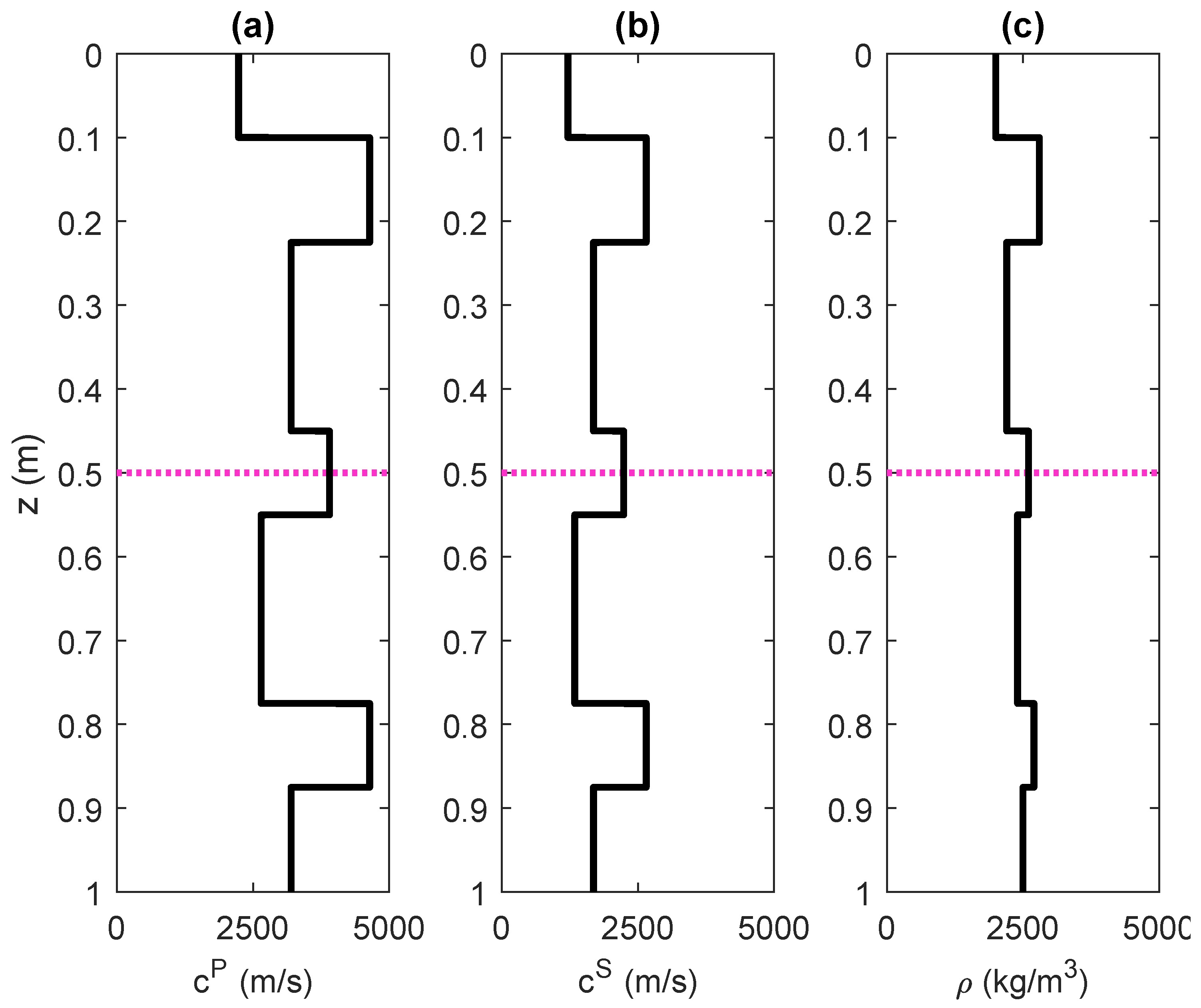
In Figure 1, we show a layered elastic medium, which will be used throughout our paper as a running example. For convenience, we have chosen the vertical dimension of the model to be 1 m. However, all quantities can be rescaled to fit a particular application in, e.g., ultrasound or seismology applications.More information on the design of the medium and the parameters that are used for modeling are provided in Appendix A. Our objective is to retrieve the Green’s responses at and to a Green’s source at a specified depth level (see the dashed magenta line in Figure 1) from recorded (reflection and transmission) data. These Green’s functions are represented by the following matrix:
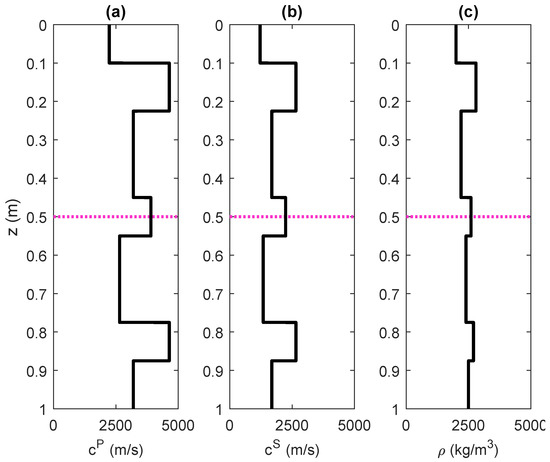
Figure 1.
Example of a layered elastic medium with (a) P-wave velocity (in m·s), (b) S-wave velocity (in m·s) and (c) density (in kg·m) as a function of depth z (in m). Above = 0 m and below = 1 m, the medium is homogeneous. The dashed magenta line indicates the focusing depth = 0.5 m, where a virtual source is to be constructed.
Here, and are the upgoing (indicated by the first superscript −) Green’s functions at from a down- and upwards radiating (indicated by the second superscript + or −) virtual source at , respectively. These quantities contain distinguished -, -, - and -components and are organized as
Here, subscripts and indicate the P- and S-wave responses to a P-wave source, whereas subscripts and indicate the P- and S-wave responses to an S-wave source. Matrices and in Equation (1) represent the downgoing Green’s functions at from an up- and downwards-radiatingvirtual source at , and are organized akin to Equation (2).
For the representations of Green’s functions, we make use of so-called focusing functions [13], which are represented by the matrix
Here, and are the up- and downgoing focusing functions (organized akin to Equation (2) at . These functions are defined in a fictitious medium where the halfspace below is homogeneous. They focus ‘from above’ at and continue as a downgoing wavefield below this depth level (see [15] for details). Similarly, and are the down- and upgoing focusing functions at . These functions are defined in a medium where the halfspace above is homogeneous. These functions focus `from below’ at and continue as an upgoing wavefield above this depth level. Finally, is an operator that reverses the signs of p and . For example, applying this operator to yields
Our objective is to retrieve the focusing functions and Green’s functions from reflection and transmission data, to be acquired at and . Let , , and be the -, -, - and -reflection responses at (for their definitions, see Appendix B.1). Based on these recordings, we can construct an operator that convolves a wavefield with the reflection response. When applied to , this multidimensional convolution is defined as
Similar operators , and can be constructed for convolution with the reflection response at , the transmission response from to and the transmission response from to , respectively. Apart from , , , and , we make use of two window operators that will be defined in the following section.
2.2. Causality Cones of Green’s Functions and Focusing Functions
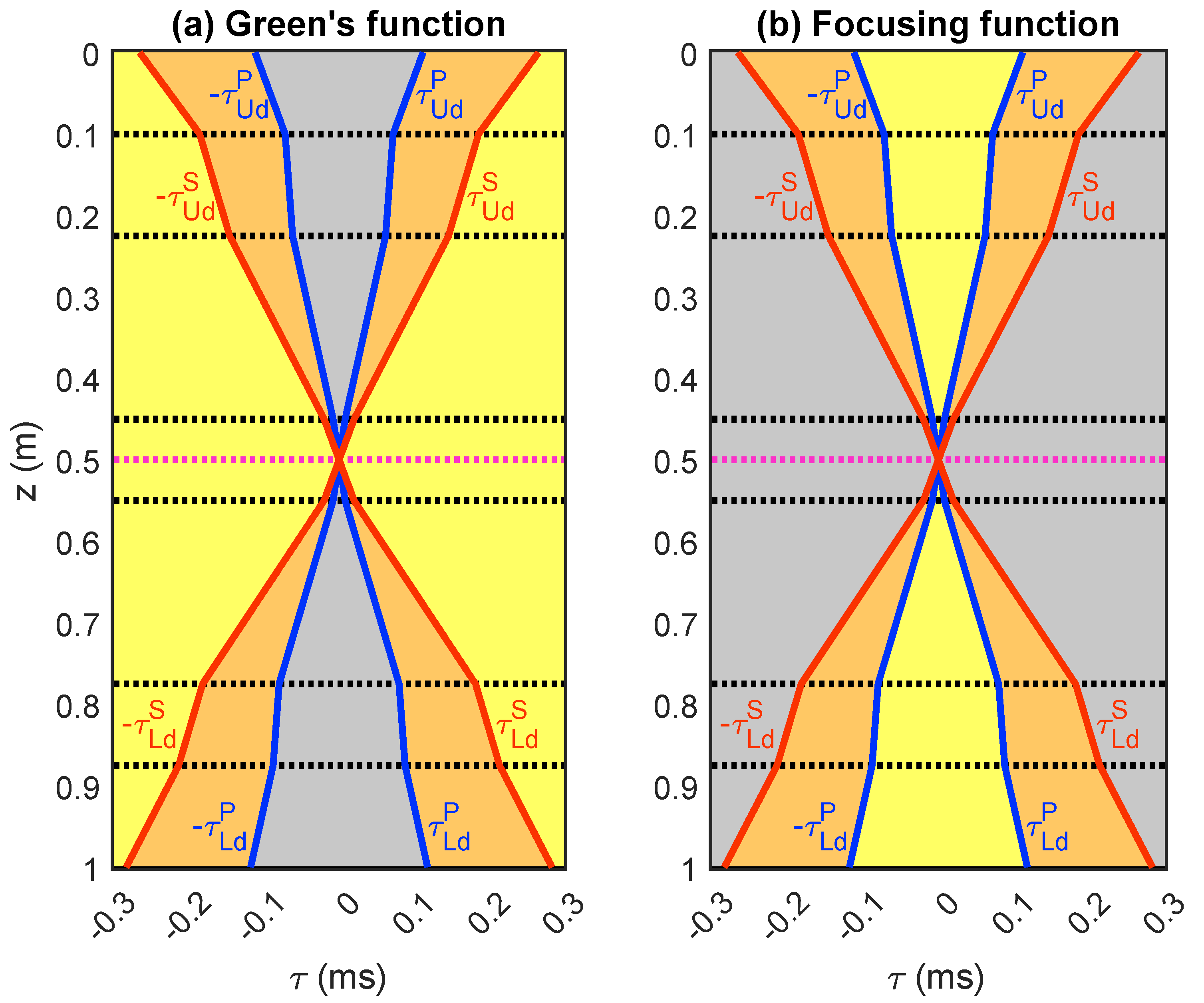
In moderately inhomogeneous acoustic media, the Green’s function and the focusing function are separated in time, except for a single overlapping event, which is commonly referred to as the direct wave. In the derivation of the acoustic Marchenko equation, this observation is exploited by truncating wavefields either before [2,11] or after [38,39] the direct wave. In elastic media, there can be a multitude of overlapping events, making the situation significantly more cumbersome [16]. To illustrate this problem, we show the (symmetrized) causality cones of multi-component Green’s functions and focusing functions in Figure 2. In particular, we refer the reader to the orange areas, where the Green’s functions and focusing functions may overlap. Because of this potential overlap, we have designed two distinct time window operators: one for Green’s functions, which is based on the (non-converted) direct P-wave travel time and one for focusing functions, which is based on the (non-converted) direct S-wave travel time .
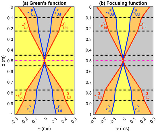
Figure 2.
Symmetrized causality cone of (a) a Green’s function ( or ) and (b) a focusing function for the medium in Figure 1 at p = 0.2 ms·m, with the source/focal depth at = 0.5 m (indicated by the magenta dashed line; the black dashed lines indicate layer boundaries). The blue lines denote the travel times and of the direct (non-converted) P-wave transmissions. The red lines denote the travel times and of the direct (non-converted) S-wave transmissions. All wavefields are stricly zero in the gray areas (whereas they may be non-zero in the yellow and orange areas). The areas where the Green’s functions and focusing functions can overlap are indicated in orange.
First, we discuss the window operator for Green’s functions, which is based on the travel time of the (non-converted) P-wave, propagating from outwards. In Figure 2a, we can see that the Green’s function and its time-reversed counterpart vanish in the interval . Let and be the components of and that reside at the boundary of the interval (corresponding to the direct non-converted P-wave transmissions). Now, we can partition the Green’s function that we defined earlier in Equation (1) as
where and are referred to as the Green’s function codasand is a zero matrix. We design a window matrix that removes all data outside the interval . When we apply this matrix to the Green’s function in Equation (6), it follows that
In this formulation, and are operators that remove all data outside the intervals and , respectively. Here, and are the direct P-wave travel times for propagation from to and , respectively.
We proceed with the window operator for focusing functions, which is based on the travel time of the (non-converted) direct S-wave, propagating from outwards. As illustrated in Figure 2b, the focusing functions and their time-reversed counterparts vanish outside . Let and be the components of and that reside at the boundary of the interval (corresponding to the direct non-converted S-wave transmissions). Now, we may partition the focusing function that we defined earlier in Equation (3) as
where and are referred to as the focusing function codas. We design a window matrix that removes all data outside the interval . During the inversion that will be applied later in this paper, we wish to restrict to the interval . To enforce this in practice, we replace in Equation (8) with , leading to
In this formulation, and are operators that remove all data outside the intervals and , respectively. Here, and are the direct S-wave travel times for propagation from to and , respectively.
2.3. Marchenko Equations
In Appendix B.1, we derive the following system of Green’s function representations that are based on reflection data:
where is a identity matrix. When we apply the operator to both sides of this equation, it follows, with the help of Equation (7), that
Next, we may substitute Equation (9) and rewrite the result as
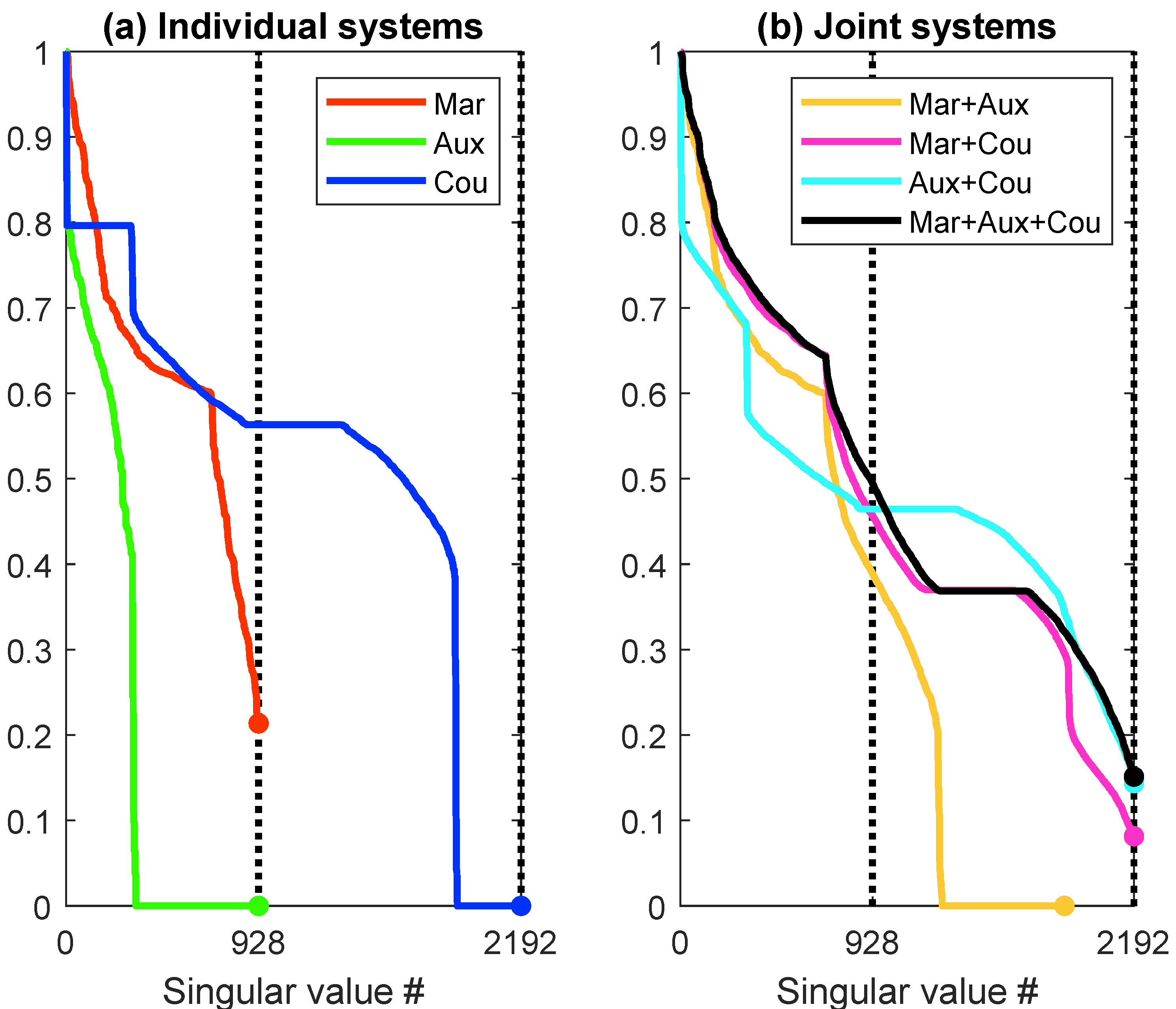
Here, we have used the fact that , such that and . We refer to Equation (12) as a system of reflection-based Marchenko equations, which could be inverted for the unknown components of the focusing function . The block-diagonal structure of this system reveals that the Marchenko equations at and are decoupled. Operator restricts the unknown focusing function to the interval . Matrix projects to the interval . As , this leads to an underdetermined system of equations, which cannot be unconditionally inverted. We illustrate this by plotting the singular values of in Figure 3a (red curve) for data from the model that we presented above in Figure 1. In this case, contains 2192 columns but only 928 independent rows. To increase the rank of this matrix, we propose to use auxiliary transmission data, for which we derive a similar system of equations in the following section.
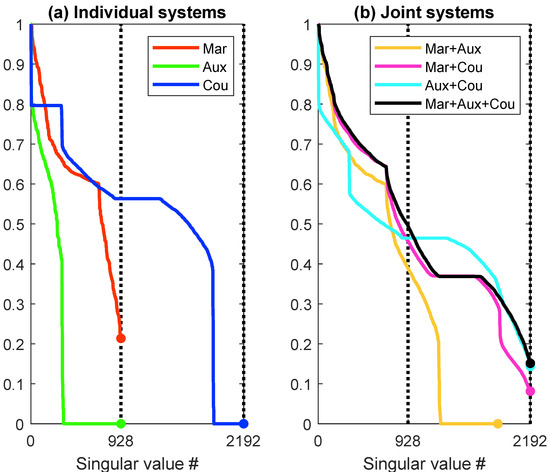
Figure 3.
(a) Singular values of the matrices (size: ), (size: ) and (size: 16,384 ) for the model in Figure 1 at p = 0.2 ms · m. (b) Singular values after concatenating various combinations of the matrices in (a). All curves have been normalized with respect to the highest singular value. The dots indicate the lowest singular values in the matrices.
2.4. Auxiliary Equations
In Appendix B.2, we derive the following system of Green’s function representations that are based on transmission data:
When we apply operator to both sides of this equation, it follows, with the help of Equation (7), that
When we substitute Equation (9), we find eventually that
We refer to 15 as a system of auxiliary equations, which can be interpreted as a transmission-based inverse problem for . In Figure 3a (green curve), we show that the governing matrix of this problem is rank-deficient (at least for the medium in Figure 1). Nevertheless, this matrix can provide complementary information to , as illustrated in Figure 3b (orange curve). In this case, we have concatenated the rows of and , leading to a matrix of rank . However, the rank is still far below 2192, which is the number of unknowns for this problem. In the next section, we show how we can improve on this by coupling reflection and transmission data, leading to yet another system of equations.
2.5. Coupled Equations
It is observed that the Green’s function matrix can be eliminated from the reflection- and transmission-based representations by subtracting Equation (13) from Equation (10). This leads to
Here, we divided by a factor 2 to achieve a better amplitude balance with the matrices that were derived in the previous sections. After the substitution of Equation (9), we obtain
We refer to 17 as a system of coupled equations, which can be interpreted as another inverse problem for . Although we have increased the number of rows signficantly (up to 16,384 in our running example) by not applying the window operator , the matrix is still rank-deficient, as shown in Figure 3a (blue curve). However, adding the rows of either or to the rows of results in a full-rank matrix, as illustrated by the magenta and cyan curves in Figure 3b. An intuitive understanding of this observation is that the subtraction of Equation (13) from Equation (10) (which was required for the construction of ) has reduced the row space of our system matrix, which can be compensated for by adding complementary rows from either the Marchenko or auxiliary system.
2.6. Joint System of Equations
Although the concatenation of matrix and either or seems sufficient by itself to construct a full-rank matrix, we choose to merge all three matrices, leading to the overall system
As indicated by the black curve in Figure 3b, matrix has full rank, and hence can be inverted. When we apply singular-value decomposition and define the pseudo-inverse as (where contains the reciprocals of all non-zero singular values), we may now write . Akin to the acoustic Marchenko problem, a range of alternative solvers can be used to compute the pseudo-inverse [40,41].
2.7. Construction of Green’s Functions from Focusing Functions
Either (the reflection-based) Equation (10) or (the transmission-based) Equation (13) can be used to convert focusing functions into Green’s functions. Alternatively, we may take the average of both approaches, leading to
We use this result later in this paper to construct Green’s functions from (retrieved) focusing functions.
3. Inversion
In order to construct matrix in Equation (18), we require a priori knowledge of four direct arrivals: , , and . In Section 3.1, we show that these arrivals can be expressed in terms of two travel times, (for P-wave transmission from to ) and (for S-wave transmission from to ), as well as two amplitude scaling factors, and . In Section 3.2, we present a procedure to estimate these scaling factors. In Section 3.3, we apply this procedure to retrieve focusing functions and Green’s functions from numerical data.
3.1. Initialization
The direct arrival that is required for the construction of can be expressed in terms of a delayed unit pulse and an amplitude scaling factor, which we parameterize strategically as for some (yet-unknown) . This leads us to obtain
The direct arrival, , that is required for the construction of can be related to by the convolutional model . Here, is the first event of the -component of the recorded transmission response from to . We assume that this event can be isolated from the transmission data by means of a time gate. Next, we define operator for the convolution of any signal with . The direct Green’s function at the lower level may now be obtained by applying to the inverse of , which can be expressed in our notation as (with as defined in Equation (20). This leads to
Similarly, the direct wave that is required for the construction of can be expressed in terms of a time-advanced unit pulse and an amplitude scaling factor, which we parameterize strategically as for some (yet-unknown) . This leads to
The direct arrival that is required for the construction of can be related to by the convolutional model . Here, is the first event of the -component of the inverse transmission response from to , which can be obtained via the inversion of , where is the autocorrelation of the source signal , as defined in Appendix A. We assume that can be isolated from by means of a time gate. Next, we define an operator for convolution with . The direct part of the focusing function at the lower level may now be obtained by applying this operator to the inverse of , which can be expressed in our notation as (with as defined in Equation (22). This leads to
We assume that the travel times and are known. The amplitude scaling factors and can be estimated from the data, as we discuss in the following section.
3.2. Estimation of Amplitude Scaling Factors and
In Appendix C, we show that the focusing function matrix can be written as an explicit function of , and , according to
In this formulation, and represent vectors, which can be explicitly computed for each value of from the recorded data (see Appendix C for details). To estimate the amplitude scaling factors and , we make use of a relation for energy conservation [42,43], which has been used earlier for the estimation of amplitude scaling factors in acoustic media [44]. This criterion can be written as
When we substitute the expressions for from (24) into (25), subtract on both sides and evaluate the result at , we find four expressions for and (i.e., the four entries of the matrix equation). The first of these expressions (corresponding to the first diagonal entry of the matrix) is independent of . We multiply this expression by and define the left-hand side of the result as . We find that
In a similar way, the last of our four expressions (corresponding to the last diagonal entry of the matrix) is independent of . We multiply this expression by and define the left-hand side of the result as . This leads to
Two more expressions can be obtained by enforcing the energy conservation of the focusing function . We find, akin to Equation (25), that
When we substitute the expressions for from Equation (24) into this result and repeat the abovementioned steps, we arrive at expressions for and (which are equivalent to Equations (26) and (27) with the subscript U replaced by L). The scaling factors and could be found by evaluating the roots of , , and . However, we have chosen an alternative approach based on minimizing the cost functions
and
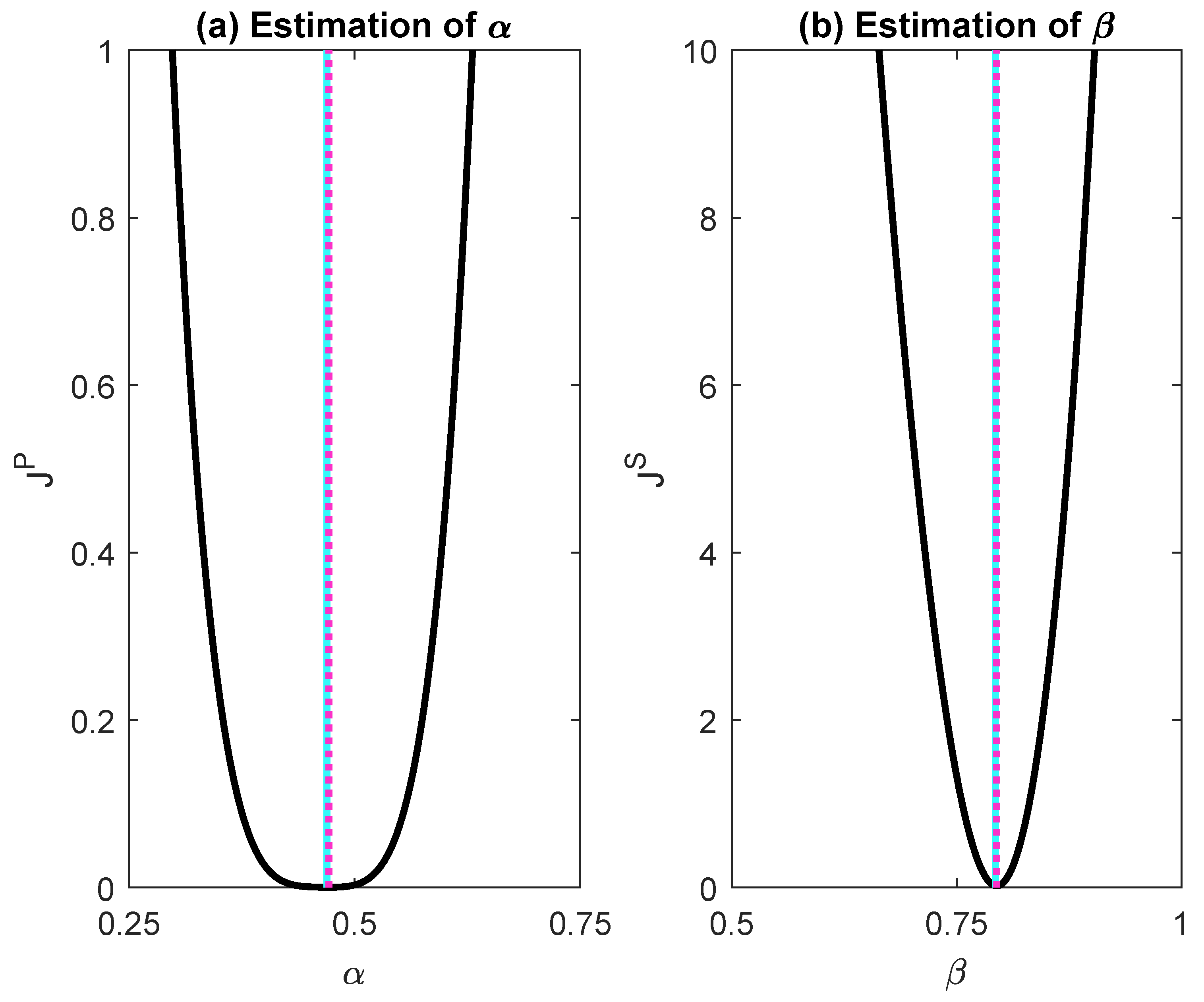
In Figure 4, we show both cost functions as computed from the numerical data of our running example. We can use Matlab’s routine to minimize these functions, yielding the estimates and (their true values being and , respectively).
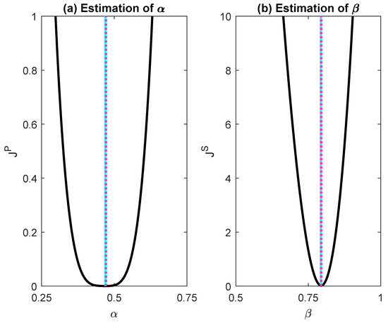
Figure 4.
Cost functions (a) and (b) for our numerical data. The dashed magenta lines denote the minima, (for ) and (for ), that were found using Matlab’s routine. The solid cyan lines denote the exact values (for ) and (for ), as extracted from the reference data.
3.3. Results
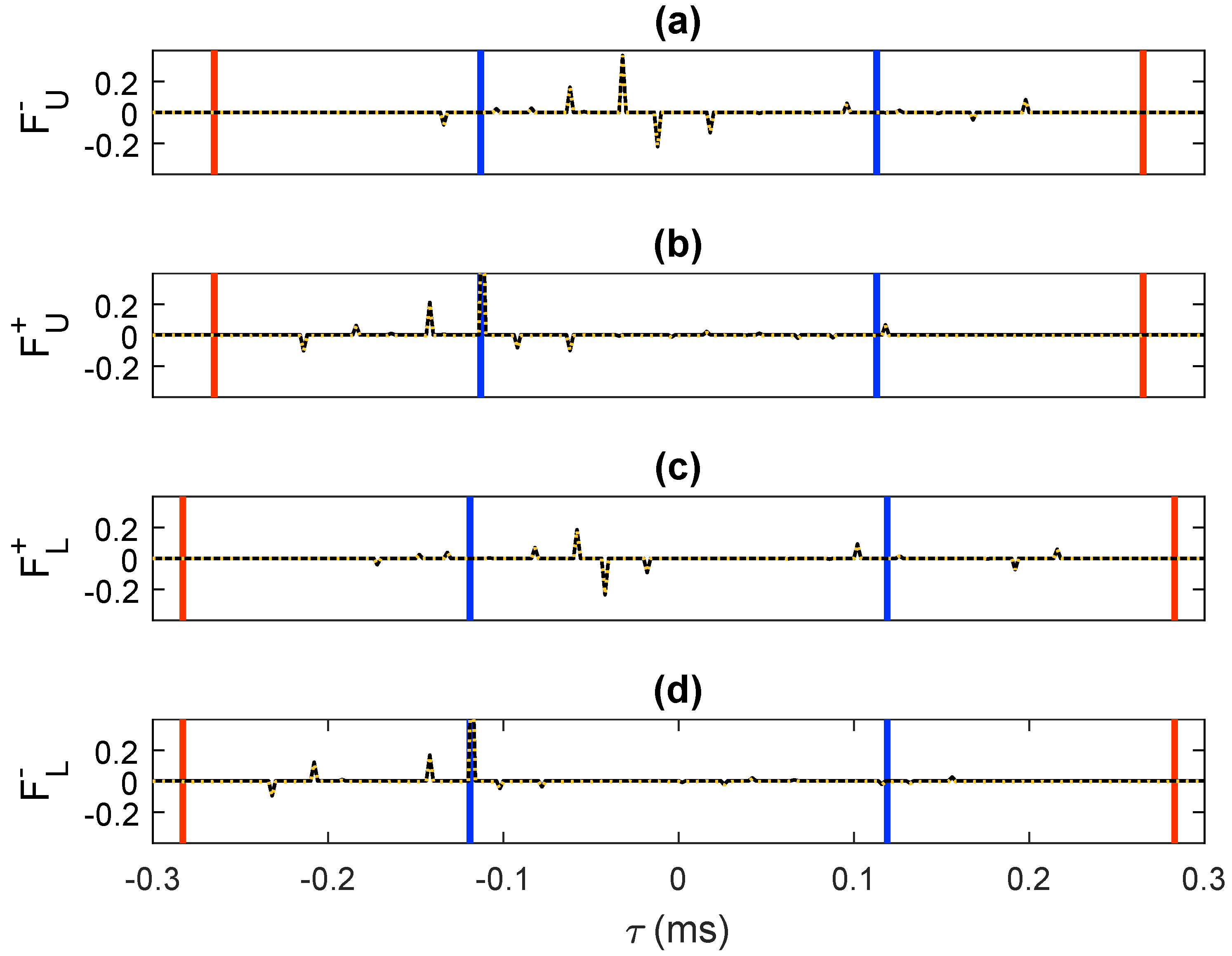
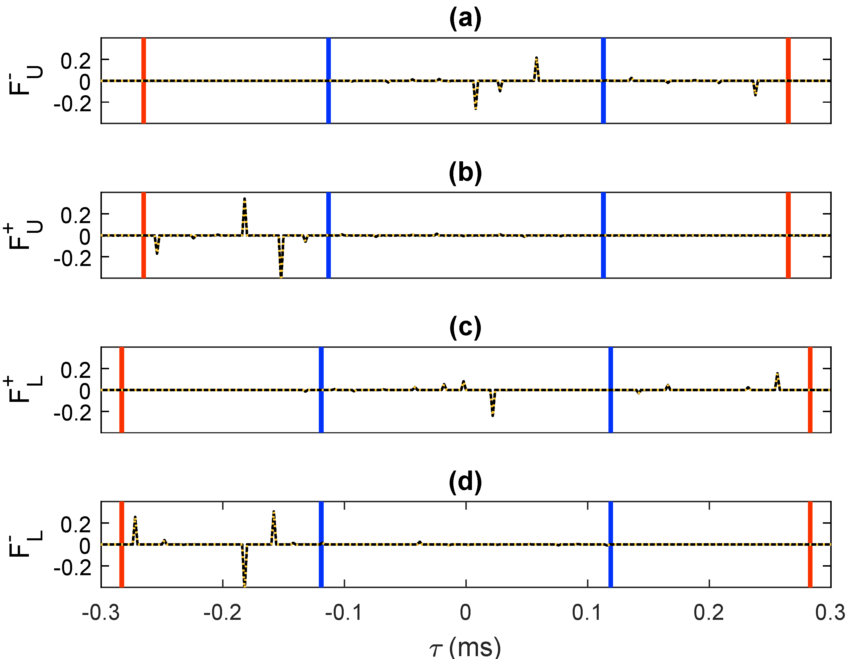
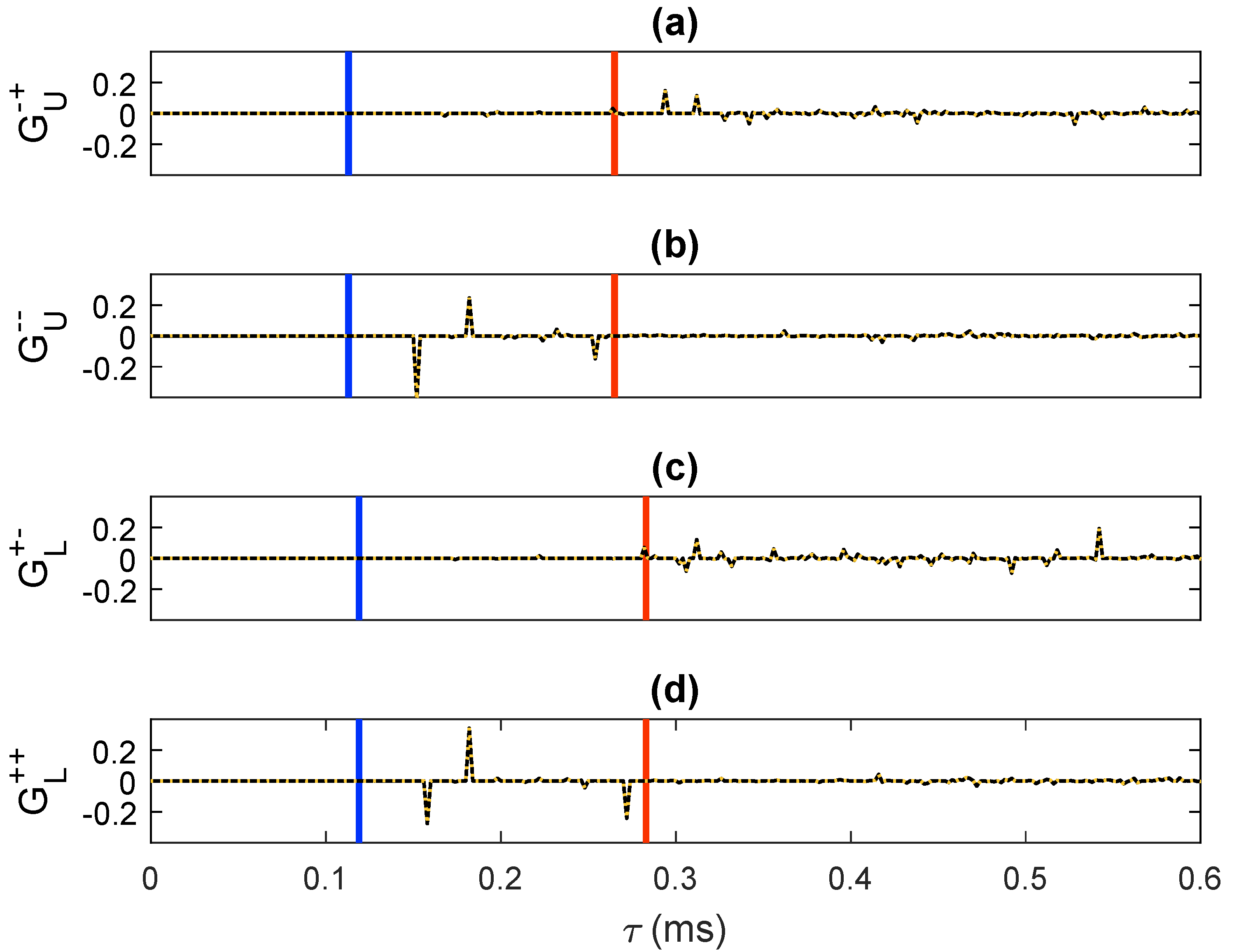
Now that and are resolved, the focusing function can be computed for our running example with the help of Equation (24). In Figure 5, Figure 6, Figure 7 and Figure 8 we compare the -, -, - and -components of the retrieved focusing functions with the results of direct modeling. We observe that all events have been recovered well, where the most significant differences (which can hardly be observed in the figure) can be attributed to the (small) errors in our estimates of and . Next, we compute the Green’s functions from the retrieved focusing functions with the help of Equation (19). In Figure 9, Figure 10, Figure 11 and Figure 12, we compare the -, -, - and -components of the retrieved Green’s functions with the results of direct modeling. Once more, we report an acceptable match, where the main differences (which can hardly be observed in the figures) can be attributed to errors in our estimates of and .
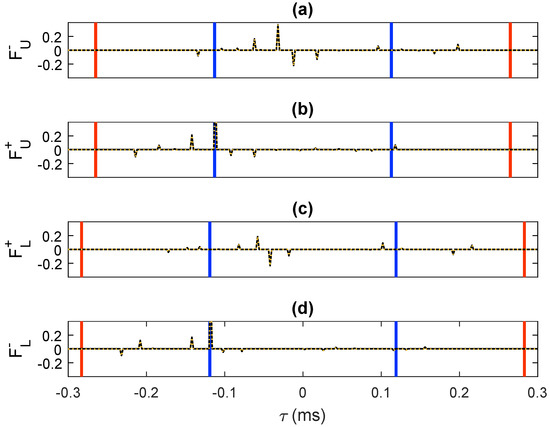
Figure 5.
-component of the retrieved focusing functions: (a) , (b) , (c) and (d) . The solid black traces were computed via direct modeling. The dashed orange traces were retrieved by means of our methodology. The blue lines have been drawn at (where s denotes the intercept time sampling) to visualize the interval . The red lines have been drawn at to visualize the interval .
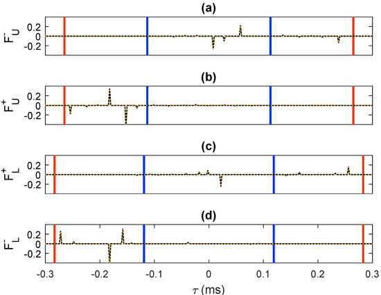
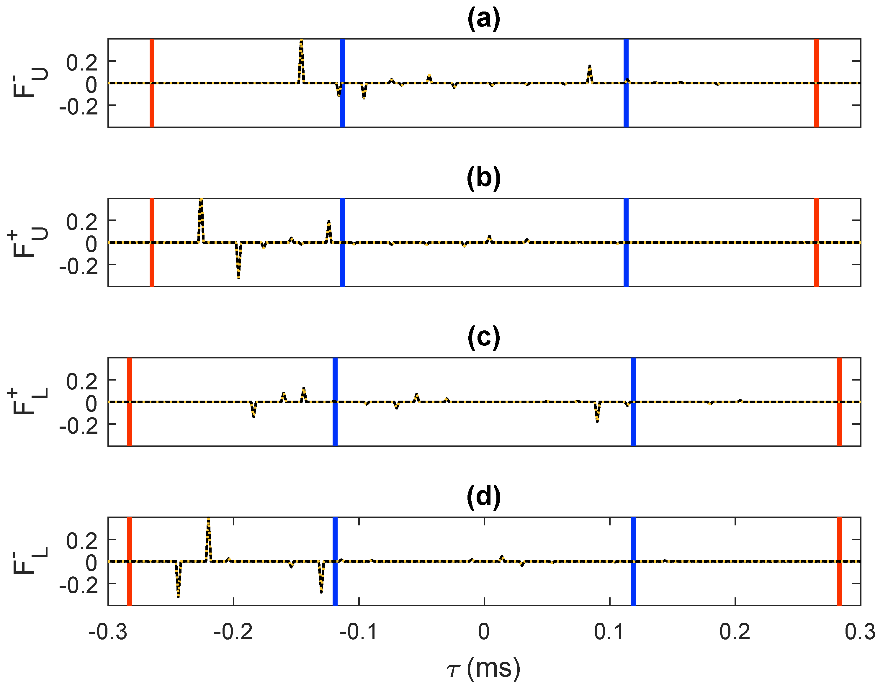
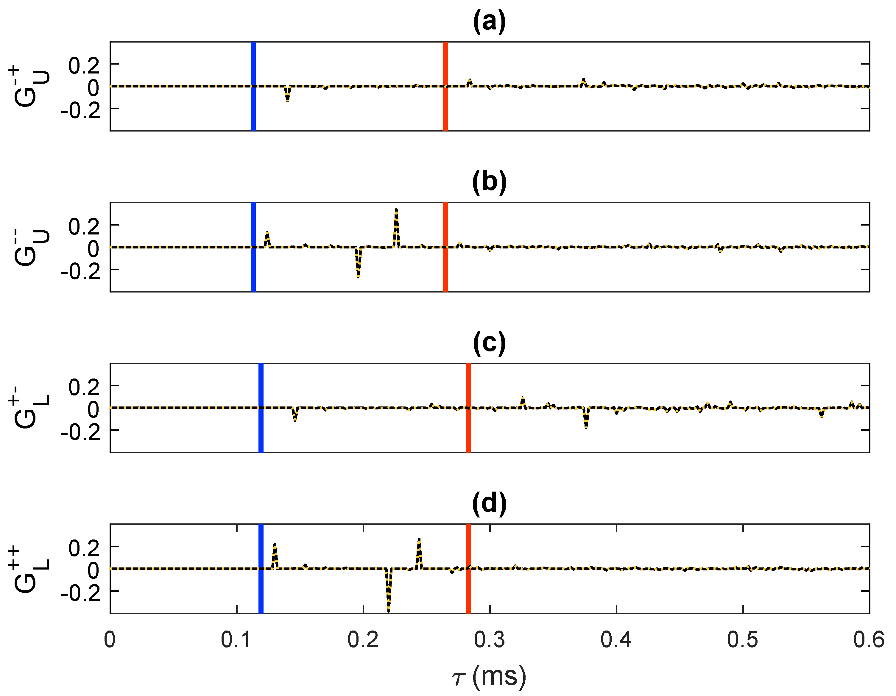
Figure 6.
-component of the retrieved focusing functions (organized as in Figure 5).
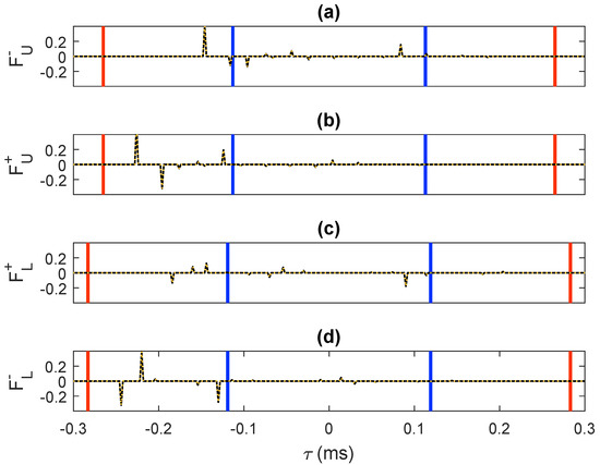
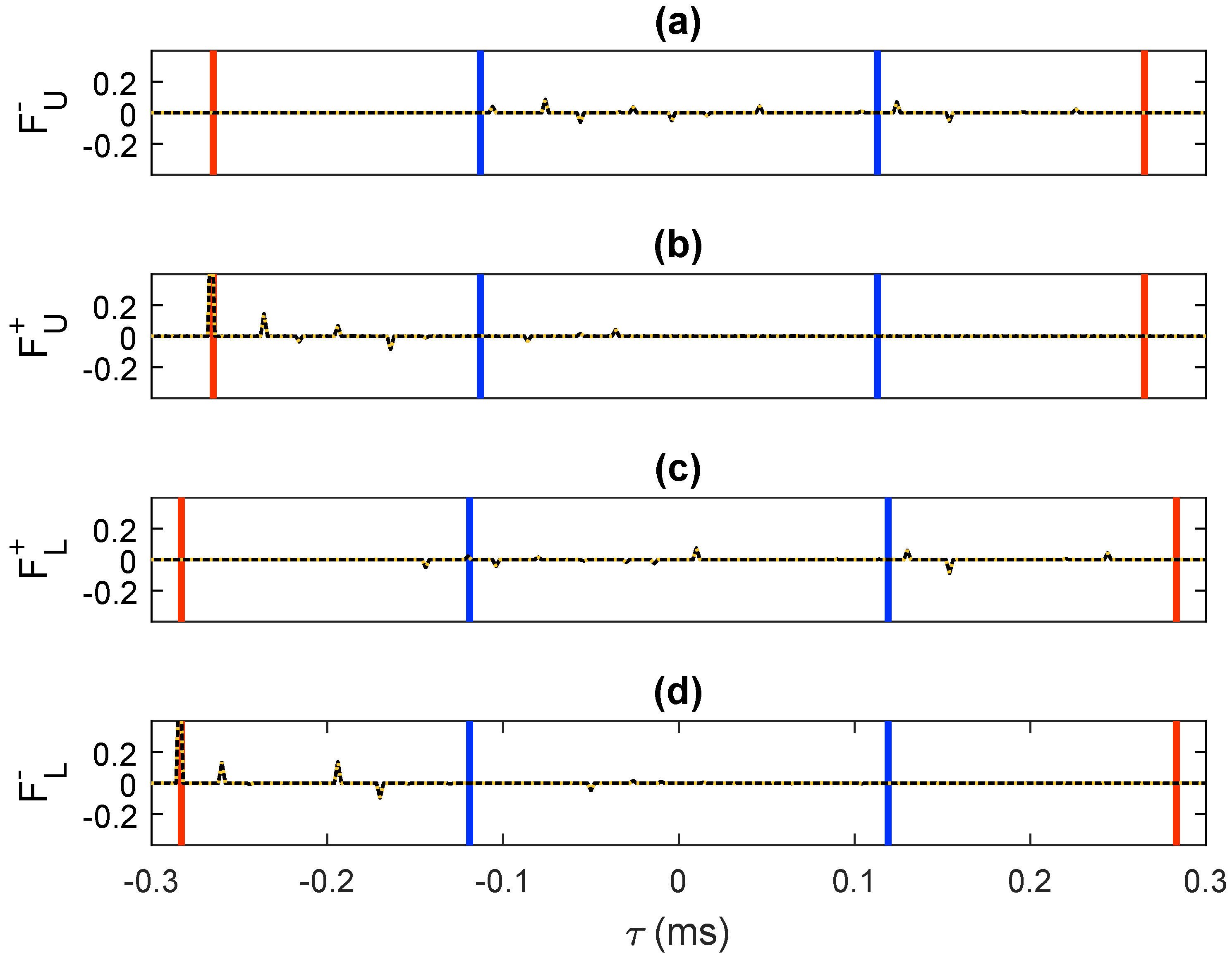
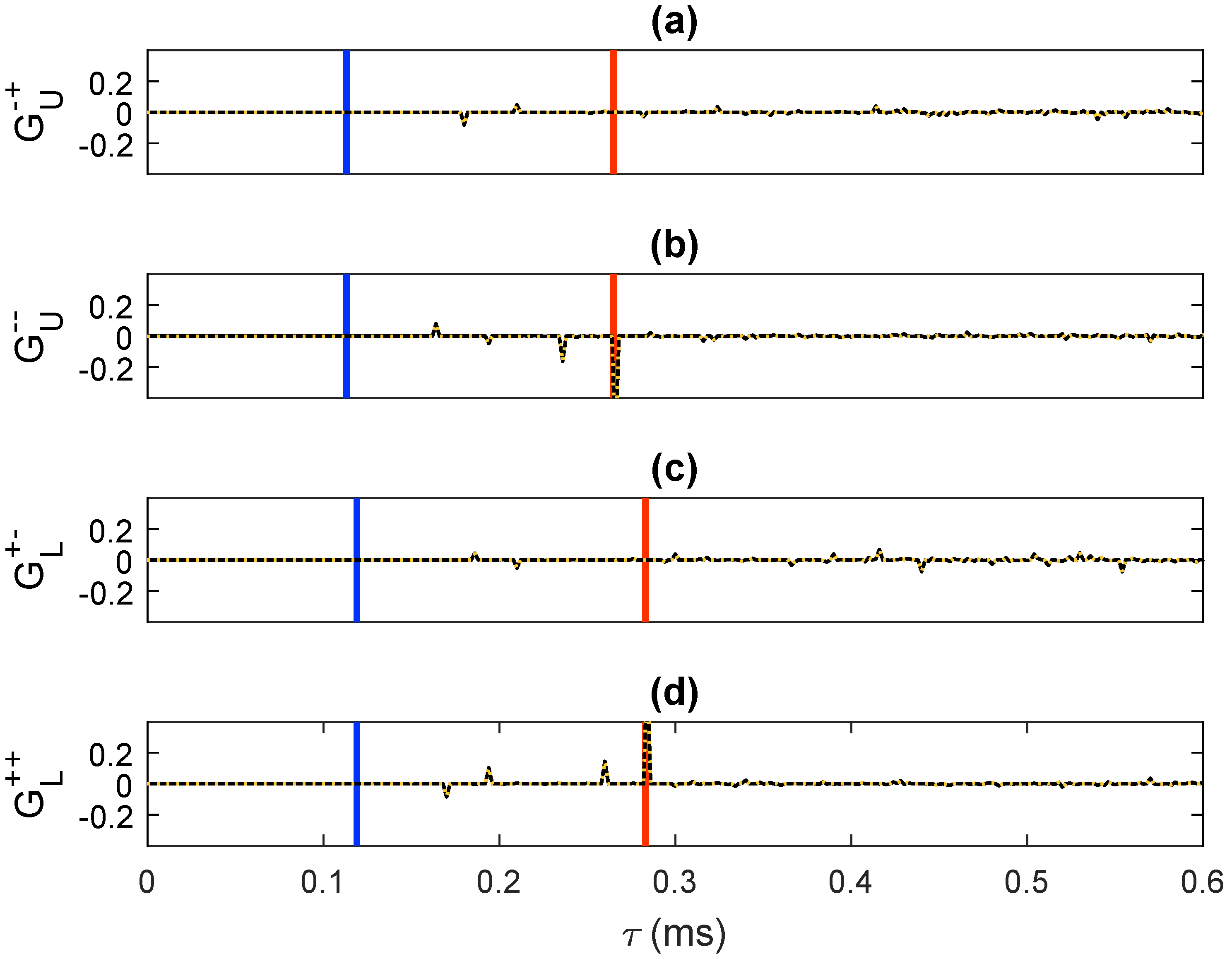
Figure 7.
-component of the retrieved focusing functions (organized as in Figure 5).
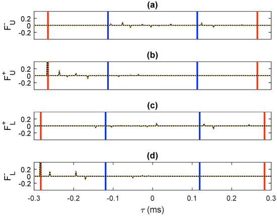
Figure 8.
-component of the retrieved focusing functions (organized as in Figure 5).
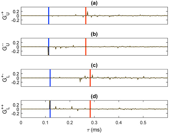
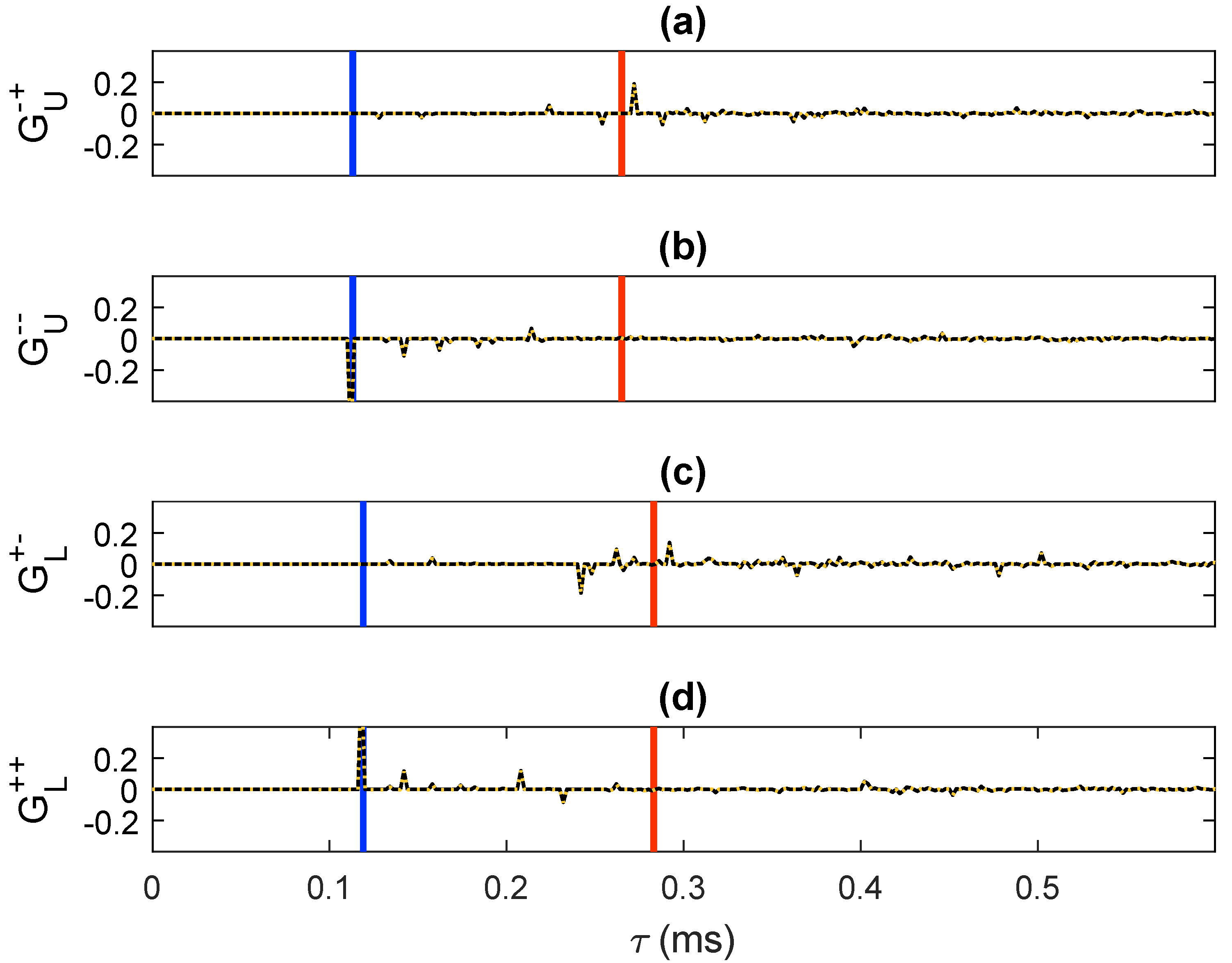
Figure 9.
-component of the retrieved Green’s functions: (a) , (b) , (c) and (d) . The solid black traces were computed via direct modeling. The dashed orange traces were retrieved using our methodology. The blue and red lines have been drawn at and , respectively.

Figure 10.
-component of the retrieved Green’s functions (organized as in Figure 9).
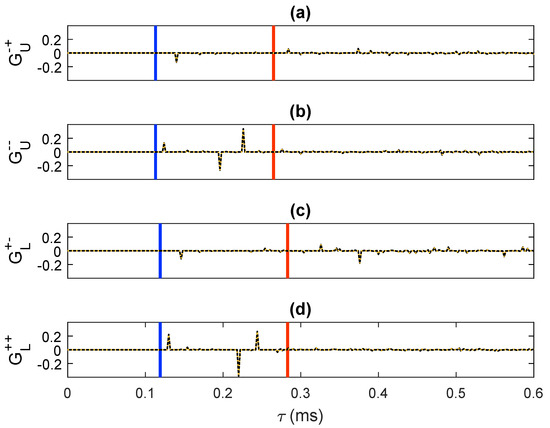
Figure 11.
-component of the retrieved Green’s functions (organized as in Figure 9).
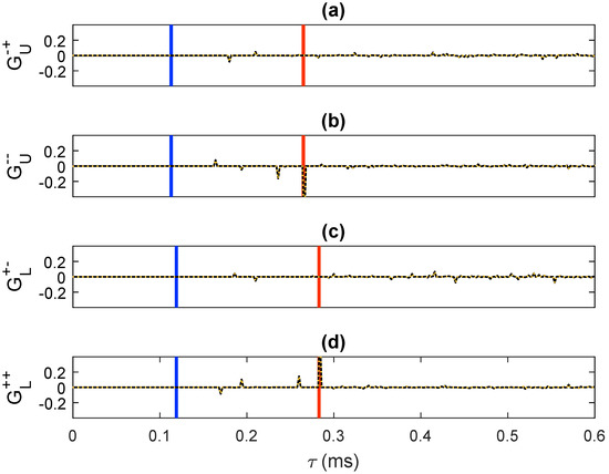
Figure 12.
-component of the retrieved Green’s functions (organized as in Figure 9).
4. Discussion
Our methodology requires knowledge of the intercept times and , whereas the focal depth may be unknown. Hence, we can effectively retrieve Green’s functions at a desired (intercept) time, even in the absence of velocity information [2]. A velocity model is only required to convert intercept times into depths, akin to acoustic Marchenko imaging [45]. An important observation in this context is that the construction of a virtual P-wave source is intrinsically decoupled from the construction of a virtual S-wave source in our formalism and both tasks may even be processed independently. Consequently, we may choose and at mutually different focal depths without affecting the accuracy of our results. Hence, we may conclude that neither and , nor the ratio , is intrinsically required for the application of our methodology.
For our numerical simulations, we have designed a medium such that the arrival times of all waveforms coincide with exact time samples (see Appendix A). In this way, we could avoid problems related to discretization. In practical applications, data are recorded within a finite frequency band only, posing limitations to our resolution, especially in the presence of thin layers [2]. It has been shown previously that some of these limitations can be overcome by enforcing energy conservation and minimum-phase conditions in the single-sided Marchenko equation [16,42,43]. Similar strategies may be applied to the system of equations that we presented in this paper.
Although our methodology has been derived for a layered lossless medium with homogeneous halfspaces above and below , it could potentially be applied to a broader range of problems. Mild lateral variations of the medium’s properties may be tolerable, akin to elastodynamic Marchenko imaging of single-sided data [12,18]. The effects of dissipation might be incorporated by computing all correlation-based reflection and transmission operators in an effectual medium, akin to the equivalent two-sided acoustic problem [33,34]. Heterogeneities above might be accounted for by convolving our representations with areal sources that take interactions with this part of the medium into account, akin to Rayleigh–Marchenko redatuming [46,47]. A similar strategy may allow us to account for heterogeneities below .
The invertibility of matrix in our formalism is likely to depend on the medium’s properties, the available bandwidth and the wavefield components that can be emitted and recorded in practice. For transcranial applications, we may modify the theory [48] or apply redatuming [49] to account for spherical arrays. Moreover, it might be necessary to place our transducers in a water layer, which is impenetrable for S-waves. In terms of matrix algebra, such a configuration induces a projection of our multi-component wavefields to a reduced domain of P-waves only [50]. It seems plausible that such a projection would affect the invertibility of , but this remains to be investigated.
5. Conclusions
We have revised the window operators in the elastodynamic Marchenko equation. This leads to a system of equations that is intrinsically rank-deficient and hence cannot be solved without additional constraints. To overcome this issue, we have introduced an auxiliary equation (based on transmission data) and a coupled equation (based on reflection and transmission data). By concatenating these equations, we can construct a joint system for two-sided data that is invertible. Apart from the reflection and transmission data, this approach requires the direct (non-converted) P- and S-wave transmission times from the focal level to the upper acquisition array and two amplitude scaling factors, which can be retrieved by enforcing energy conservation. This leads to a methodology for velocity-independent true-amplitude Green’s function retrieval in a lossless layered isotropic elastic medium from two-sided data. The methodology could potentially be extended to account for mild lateral variations, dissipation, anisotropy and heterogeneities above the upper acquisition array, as well as below the lower acquisition array.
Author Contributions
Conceptualization, J.V.d.N., J.B., G.A.M., E.S. and K.W.; Investigation, J.V.d.N.; Methodology, J.V.d.N., J.B., G.A.M., E.S. and K.W.; Supervision, E.S. and K.W.; Validation, J.V.d.N.; Visualization, J.V.d.N.; Writing—original draft, J.V.d.N.; Writing—review & editing, J.V.d.N. All authors have read and agreed to the published version of the manuscript.
Funding
This research has received funding from the European Research Council (grant no. 742703).
Institutional Review Board Statement
Not applicable.
Informed Consent Statement
Not applicable.
Data Availability Statement
Not applicable.
Conflicts of Interest
The authors declare no conflict of interest.
Appendix A. Numerical Settings
In this Appendix, we provide more information on the layered elastic medium depicted in Figure 1. We also provide the parameters that were used to generate numerical data for the running example that is discussed in the main text. Our model consisted of 41 depth samples with spacing = 25 mm. Data records were generated by modeling at a single ray parameter p = 0.2 ms·m [36]. Our traces consisted of 2048 (intercept) time samples, which were sampled with = 2 s. For the source signal , we used a discretized delta function, where the sample at equaled one and all remaining samples were zero. Inspired by [16], we chose model parameters that generated on-sample data at p = 0.2 ms·m. This was achieved by choosing velocity values as elements of the set
In Table A1, we show the specific integers and that were used for each layer k of our model, to compute the velocities and as elements of . This procedure ensured that all (primary and multiple) reflections and transmissions arrived at exact sample values in our records. We also indicate the layer thicknesses , densities , as well as the travel times and that were required for P- and S-waves to traverse each layer when p = 0.2 ms·m. We note that the medium broke the separability conditions of [16] at both and = 1 m, given the focal depth = 0.5 m (which is in layer in the model). This was due to the fact that s exceeded both s and s, whereas s exceeded both s and s.

Table A1.
Parameters used for the model shown in Figure 1.
Table A1.
Parameters used for the model shown in Figure 1.
| k | (mm) | (kg · m) | (s) | (s) | ||
|---|---|---|---|---|---|---|
| 0 | 5 | 10 | 100 | 2000 | 40 | 80 |
| 1 | 1 | 4 | 125 | 2800 | 10 | 40 |
| 2 | 3 | 7 | 225 | 2200 | 54 | 126 |
| 3 | 2 | 5 | 100 | 2600 | 16 | 40 |
| 4 | 4 | 9 | 225 | 2400 | 72 | 162 |
| 5 | 1 | 4 | 100 | 2700 | 8 | 32 |
| 6 | 3 | 7 | 125 | 2500 | 30 | 70 |
Appendix B. Derivations
In this Appendix, we derive several representations that were used in the main text. We conduct these derivations in the -domain (which is indicated by a hat), where denotes the angular frequency. We define the Fourier transform of an arbitrary (down- or upgoing) wavefield as
whereas the associated inverse Fourier transform is given by
Here, it is assumed that the signals are real-valued in the -domain and ℜ denotes the real part. Our derivations are based on two reciprocity theorems for flux-normalized wave fields, which we present for a source-free volume that is enclosed by depth levels (at the top) and (at the bottom). First, we have the reciprocity theorem of the convolution type [15]
Here, and are down- and upgoing wavefields in state A, whereas and are equivalent wavefields in state B. Furthermore, denotes matrix transposition. We have an equivalent reciprocity theorem of the correlation type [15]
where denotes the adjoint. In the following, we use Equations (A4) and (A5) to derive representations that are based on reflection and transmission data.
Appendix B.1. Reflection-Based Representations
First, we derive a convolution-based representation for reflection data at . For this purpose, we set and in Equation (A4). In state A, we use the properties of the actual medium and we place a unit source just above , such that (a identity matrix), (the reflection response `from above’ at ), (the downwgoing Green’s function at due to a downgoing source at ) and (the upgoing Green’s function at due to a downgoing source at ). In state B, we truncate the medium at and choose a homogeneous halfspace below this level. For the wavefield in this state, we choose a focusing function with a focal point at , which is purely downgoing below this level [15]. This leads to (the downgoing focusing function at ), (the upgoing focusing function at ), (the focused field at ) and . Substitution of these quantities into Equation (A4) yields
where we have used and [51]. We can derive an equivalent correlation-based representation by substituting the same quantities into Equation (A5), leading to
where we have used and [51]. Two more representation can be derived for reflection data at by choosing and in Equations (A4) and (A5) and placing a source just below . Once again, we choose the actual medium properties in state A, such that (the downgoing Green’s function at due to an upgoing source at ), (the upgoing Green’s function at due to an upgoing source at ), (the reflection response `from below’ at ) and (a identity matrix). In state B, we truncate the medium at and choose a homogeneous halfspace above this level. For the wavefield in this state, we choose a focusing function with a focal point at , which is purely upgoing above this level. This leads to , (the focused field at ), (the downgoing focusing function at ) and (the upgoing focusing function at ). Substitution of these quantities into Equation (A4) yields
where we have used and [51]. Alternatively, we may substitute the quantities into Equation (A5), leading to
where we have used and [51]. The system of Equations (A6)–(A9) can be rewritten as
where we have dropped subscript I (denoting the focal depth) for notational convenience. After taking the inverse Fourier transform (as defined in Equation (A3) and applying operator to the second and fourth rows, we obtain Equation (10), presented in the main text.
Appendix B.2. Transmission-Based Representations
We can derive a system of equivalent equations that are based on transmission data. First, we set and . We choose the actual medium in state A and place a source just below , leading to , (the transmission response from to ), and . In state B, we truncate the medium at and choose a homogeneous halfspace below this level. For the wavefield in this state, we choose a focusing function that focuses at and is purely downgoing below this level. This leads to , , and . Substituting these quantities into Equation (A4) yields
where we have used and [51]. We may substitute the same quantities into Equation (A5), leading to
where we have used and [51]. We can derive two more representations by setting and , and placing a source just above . In state A, we use the actual medium properties, leading to: , , (the transmission response from to ) and . In state B, we truncate the medium at and choose a homogeneous halfspace above this level. For the wavefield in this state, we choose a focusing function that focuses at and is purely upgoing above this level. This leads to , , and . Substituting these quantities into Equation (A4) yields
where we have used and [15]. Alternatively, the quantities can be substituted into Equation (A5), leading to
where we have used and [51]. The system of Equations (A11)–(A14) can be rewritten as
where we have dropped the subscript I once again for notational convenience. After taking the inverse Fourier transform (as defined in Equation (A3) and applying operator to the first and third row, we obtain Equation (13), presented in the main text.
Appendix C. Expression for F as a Function of τ, α and β
In this Appendix, we write explicitly as a function of , and . We start with the substitution of Equations (20)–(23) into the definition of , which is given in the left-hand side of Equation (12). We write the result as
where and have been used to identify the constructed matrices. In a similar way, we can substitute Equations (20)–(23) into the definition of , which is given in the left-hand side of Equation (15). This leads to
where and have been used to identify the constructed matrices. Finally, we may substitute Equations (22) and (23) into the definition of , which is given in the left-hand side of Equation (17). This yields
where and have been used to identify the constructed matrices. Next, we substitute Equations (A16)–(A18) into (18) and apply the pseudo-inverse of to both sides of the result. This eventually leads to
The direct focusing function matrix can be written in a similar form. This is achieved by substituting Equations (22) and (23) into the definition of , which is given in the right-hand side of Equation (8). The result can strategically be written as
Here, we have indicated the arguments of all matrices for convenience to emphasize that we have expressed explicitly as a function of , and . Note that and are independent ofthe scaling factors and hence can be computed from the recorded data, and . Finally, we can express our result as Equation (24), presented in the main text, by renaming the quantities that constitute matrices and .
References
- Broggini, F.; Snieder, R. Connection of scattering principles: A visual and mathematical tour. Eur. J. Phys. 2012, 33, 593–613. [Google Scholar]
- Slob, E.; Wapenaar, K.; Broggini, F.; Snieder, R. Seismic reflector imaging using internal multiples with Marchenko-type equations. Geophysics 2014, 79, S63–S76. [Google Scholar]
- Cui, T.; Vasconcelos, I.; van Manen, D.-J.; Wapenaar, K. A tour of Marchenko redatuming: Focusing the subsurface wavefield. Lead. Edge 2018, 37, 67a1–67a6. [Google Scholar]
- Lomas, A.; Curtis, A. An introduction to Marchenko methods for imaging. Geophysics 2019, 84, F35–F45. [Google Scholar]
- Thorbecke, J.; Slob, E.; Brackenhoff, J.; van der Neut, J.; Wapenaar, K. Implementation of the Marchenko method. Geophysics 2017, 82, WB29–WB45. [Google Scholar]
- Ravasi, M.; Vasconcelos, I. An open-source framework for the implementation of large-scale integral operators with flexible, modern HPC solutions - enabling 3D Marchenko imaging by least squares inversion. Geophysics 2021, 86, WC177–WC194. [Google Scholar]
- Brackenhoff, J.; Thorbecke, J.; Meles, G.; Koehne, V.; Barrera, D.; Wapenaar, K. 3D Marchenko applications: Implementation and examples. Geophys. Prospect. 2022, 70, 35–56. [Google Scholar]
- Staring, M.; Pereira, R.; Douma, H.; van der Neut, J.; Wapenaar, K. Source-receiver Marchenko redatuming on field data using an adaptive double-focusing method. Geophysics 2018, 83, S579–S590. [Google Scholar]
- Zhang, L.; Slob, E. A field data example of Marchenko multiple elimination. Geophysics 2020, 85, S65–S70. [Google Scholar]
- Jia, X.; Baumstein, A.; Jing, C.; Neumann, E.; Snieder, R. Subsalt Marchenko imaging with offshore Brazil field data. Geophysics 2021, 86, WC31–WC40. [Google Scholar]
- Wapenaar, K.; Brackenhoff, J.; Dukalski, M.; Meles, G.; Reinicke, C.; Slob, E.; Staring, M.; Thorbecke, J.; van der Neut, J.; Zhang, L. Marchenko redatuming, imaging, and multiple elimination and their mutual relations. Geophysics 2021, 86, WC117–WC140. [Google Scholar]
- da Costa Filo, C.A.; Ravasi, M.; Curtis, A.; Meles, G.A. Elastodynamic Green’s function retrieval through single-sided Marchenko inverse scattering. Phys. Rev. E 2014, 90, 063201. [Google Scholar]
- Wapenaar, K. Single-sided Marchenko focusing of compressional and shear waves. Phys. Rev. E 2014, 90, 063202. [Google Scholar]
- Wapenaar, K.; Snieder, R.; de Ridder, S.; Slob, E. Green’s function representation for Marchenko imaging without up/down decomposition. Geophys. J. Int. 2021, 227, 184–203. [Google Scholar]
- Wapenaar, K.; Slob, E. On the Marchenko equation for multicomponent single-sided reflection data. Geophys. J. Int. 2014, 199, 1367–1371. [Google Scholar]
- Reinicke, C.; Dukalski, M.; Wapenaar, K. Comparison of monotonicity challenges encountered by the inverse scattering series and the Marchenko demultiple method for elastic waves. Geophysics 2020, 85, Q11–Q26. [Google Scholar]
- Reinicke, C.; Wapenaar, K. Elastodynamic single-sided homogeneous Green’s function representation: Theory and numerical examples. Wave Motion 2019, 89, 245–264. [Google Scholar]
- da Costa Filho, C.; Ravasi, M.; Curtis, C. Elastic P- and S-wave autofocus imaging with primaries and internal multiples. Geophysics 2015, 80, S187–S202. [Google Scholar]
- da Costa Filho, C.; Meles, G.A.; Curtis, C. Elastic internal multiple analysis and attenuation using Marchenko and interferometric medhods. Geophysics 2017, 82, Q1–Q12. [Google Scholar]
- Thomsen, H.R.; Molerón, M.; Haag, T.; van Manen, D.-J.; Robertsson, J.O.A. Elastic immersive wave experimentation: Theory and physical implementation. J. Phys. Rev. Res. 2019, 1, 033203. [Google Scholar]
- Niederleithinger, E.; Wolf, J.; Mielentz, F.; Wiggenhauser, H.; Pirskawetz, S. Embedded ultrasonic transducers for active and passive concrete monitoring. Sensors 2015, 15, 9756–9772. [Google Scholar]
- Bazulin, E.; Goncharsky, A.; Romanov, S.; Seryozhnikov, S. Ultrasound transmission and reflection tomography for nondestructive testing using experimental data. Ultrasonics 2022, 124, 106765. [Google Scholar]
- Taskin, U.; Eikrem, K.S.; Nævdal, G.; Jakobsen, M.; Verschuur, D.J.; van Dongen, K.W.A. Ultrasound imaging of the brain using full-waveform inversion. In Proceedings of the 2020 IEEE International Ultrasonics Symposium (IUS), Las Vegas, NV, USA, 7–11 September 2020. [Google Scholar]
- Marty, P.; Boehm, C.; Fichtner, A. Acoustoelastic full-waveform inversion for transcranial ultrasound computed tomography. In Proceedings of the SPIE Medical Imaging 2021, Online, 15–20 February 2021. [Google Scholar]
- Meles, G.A.; van der Neut, J.; van Dongen, K.W.A.; Wapenaar, K. Wavefield finite time focusing with reduced spatial exposure. J. Acoust. Soc. Am. 2019, 145, 3521–3530. [Google Scholar]
- Brackenhoff, J.; van der Neut, J.; Meles, G.; Marty, P.; Boehm, C. Virtual ultrasound transducers in the human brain. In Proceedings of the SPIE Medical Imaging 2022, San Diego, CA, USA, 20 February–28 March 2022. [Google Scholar]
- Na, S.; Yuan, X.; Lin, L.; Isla, J.; Garrett, D.; Wang, L.V. Transcranial photoacoustic computed tomography based on a layered back-projection method. Photoacoustics 2020, 20, 100213. [Google Scholar]
- Poudel, J.; Na, S.; Wang, L.V.; Anastasio, M.A. Iterative image reconstruction in transcranial photoacoustic tomography based on the elastic wave equation. Phys. Med. Biol. 2020, 65, 055009. [Google Scholar]
- Liu, Y.; van der Neut, J.; Arntsen, B.; Wapenaar, K. Combination of surface and borehole seismic data for robust target-oriented imaging. Geoph. J. Int. 2016, 205, 758–775. [Google Scholar]
- Lomas, A.; Singh, S.; Curtis, A. Imaging vertical structures using Marchenko methods with vertical seismic-profile data. Geophysics 2020, 85, S103–S113. [Google Scholar]
- Singh, S.; Snieder, R.; van der Neut, J.; Thorbecke, J.; Slob, E.; Wapenaar, K. Accounting for free-surface multiples in Marchenko imaging. Geophysics 2017, 82, R19–R30. [Google Scholar]
- Dukalski, M.; de Vos, K. Marchenko inversion in a strong scattering regime including surface-related multiples. Geophys. J. Int. 2018, 212, 760–776. [Google Scholar]
- Slob, E. Green’s function retrieval and Marchenko imaging in a dissipative acoustic medium. Phys. Rev. Lett. 2016, 116, 164301. [Google Scholar]
- Cui, T.; Becker, T.S.; van Manen, D.J.; Rickett, J.E.; Vasconcelos, I. Marchenko redatuming in a dissipative medium: Numerical and experimental implementation. Phys. Rev. Appl. 2018, 19, 044022. [Google Scholar]
- Frasier, C.W. Discrete time solution of plane P-SV waves in a plane layered medium. Geophysics 1970, 35, 197–219. [Google Scholar]
- Kennett, B.L.N. Seismic Wave Propagation in Stratified Media; Cambridge University Press: Cambridge, UK, 1983. [Google Scholar]
- Schalkwijk, K.M.; Wapenaar, C.P.A.; Verschuur, D.J. Adaptive decomposition of multicomponent ocean-bottom seismic data into downgoing and upgoing P- and S-waves. Geophysics 2003, 68, 1091–1102. [Google Scholar]
- Zhang, L.; Slob, E.; van der Neut, J.; Wapenaar, K. Artifact-free reverse time migration. Geophysics 2018, 83, A65–A68. [Google Scholar]
- Diekmann, L.; Vasconcelos, I. Focusing and Green’s function retrieval in three-dimensional inverse scattering revisited: A single-sided Marchenko integral for the full wave field. Phys. Rev. Res. 2021, 3, 013206. [Google Scholar]
- Slob, E.; Zhang, L. Unified elimination of 1D acoustic multiple reflection. Geophys. Prospect. 2021, 69, 327–348. [Google Scholar]
- Santos, R.S.; Revelo, D.E.; Pestana, R.C.; Koehne, V.; Barrera, D.F.; Souza, M.S. An application of the Marchenko internal multiple elimination scheme formulated as a least-squares problem. Geophysics 2021, 86, WC105–WC116. [Google Scholar]
- Dukalski, M.; Mariani, E.; de Vos, K. Handling short-period scattering using augmented Marchenko autofocusing. Geophys. J. Int. 2019, 216, 2129–2133. [Google Scholar]
- Elison, P.; Dukalski, M.S.; de Vos, K.; van Manen, D.J.; Robertsson, J.O.A. Data-driven control over short-period internal multiples in media with a horizontally layered overburden. Geophys. J. Int. 2020, 221, 769–787. [Google Scholar]
- Mildner, C.; Dukalski, M.; Elison, P.; de Vos, K.; Broggini, F.; Robertsson, J.O.A. True-amplitude-versus-offset Green’s function retrieval using augmented Marchenko focusing. In Proceedings of the 81st EAGE Conference & Exhibition 2019, London, UK, 3–6 June 2019. [Google Scholar]
- Sripanich, Y.; Vasconcelos, I.; Wapenaar, K. Velocity-independent Marchenko focusing in time- and depth-imaging domains for media with mild lateral heterogeneity. Geophysics 2019, 84, Q57–Q72. [Google Scholar]
- Ravasi, M. Rayleigh-Marchenko redatuming for target-oriented, true-amplitude imaging. Geophysics 2017, 82, S439–S452. [Google Scholar]
- Vargas, D.; Vasconcelos, I.; Sripanich, Y.; Ravasi, M. Scattering-based focusing for imaging in highly complex media from band-limited, multicomponent data. Geophysics 2021, 86, WC141–WC157. [Google Scholar]
- Brackenhoff, J.; van der Neut, J.; Marty, P. Creating virtual measurements inside a medium using spherical recording arrays. In Proceedings of the AGU Fall Meeting 2021, New Orleans, LA, USA, 13–17 December 2021. [Google Scholar]
- Taskin, U.; van der Neut, J.; Gemmeke, H.; van Dongen, K.W.A. Redatuming of 2-D wavefields measured on an arbitrary-shaped closed aperture. IEEE Trans. Ultrason. Ferroelectr. Freq. Control 2019, 67, 173–179. [Google Scholar]
- Reinicke, C.; Dukalski, M.; Wapenaar, K. Internal multiple elimination: Can we trust an acoustic approximation? Geophysics 2021, 86, WC41–WC54. [Google Scholar]
- Wapenaar, C.P.A. One-way representations of seismic data. Geophys. J. Int. 1996, 127, 178–188. [Google Scholar]
Publisher’s Note: MDPI stays neutral with regard to jurisdictional claims in published maps and institutional affiliations. |
© 2022 by the authors. Licensee MDPI, Basel, Switzerland. This article is an open access article distributed under the terms and conditions of the Creative Commons Attribution (CC BY) license (https://creativecommons.org/licenses/by/4.0/).