Novel Unbiased Optimal Receding-Horizon Fixed-Lag Smoothers for Linear Discrete Time-Varying Systems

Abstract

This paper proposes novel unbiased minimum-variance receding-horizon fixed-lag (UMVRHF) smoothers in batch and recursive forms for linear discrete time-varying state space models in order to improve the computational efficiency and the estimation performance of receding-horizon fixed-lag (RHF) smoothers. First, an UMVRHF smoother in batch form is proposed by combining independent receding-horizon local estimators for two separated sub-horizons. The local estimates and their error covariance matrices are obtained based on an optimal receding horizon filter and the smoother in terms of the unbiased minimum variance; they are then optimally combined using Millman’s theorem. Next, the recursive form of the proposed UMVRHF smoother is derived to improve its computational efficiency and extendibility. Additionally, we introduce a method for extending the proposed recursive smoothing algorithm to a posteriori state estimations and propose the Rauch–Tung–Striebel receding-horizon fixed-lag smoother in recursive form. Furthermore, a computational complexity reduction technique that periodically switches the two proposed recursive smoothing algorithms is proposed. The performance and effectiveness of the proposed smoothers are demonstrated by comparing their estimation results with those of previous algorithms for Kalman and receding-horizon fixed-lag smoothers via numerical experiments.

1. Introduction

Fixed-lag smoothers have been widely investigated because they provide optimal estimates, unlike filters and predictors [1,2,3,4]. In practice, smoothers are often used to improve the performance of filters, provided delays can be tolerated. In smoothing problems, the objective is to estimate past or delayed states using past measurements up to the current time. Three types of smoothers exist: fixed-point, fixed-lag, and fixed-interval smoothers. The fixed-lag smoother is the most useful type because it offers more accurate and general solutions than filters. Thus, smoothers have been considered as a suitable choice in many applications where a short time delay is acceptable, such as denoising ECG signals [5], image processing [6], target tracking [7,8,9], system-on-chip testing [10], structural dynamics estimation [11,12], and vibration analysis [13].

The structures of fixed-lag smoothers can be categorized as infinite impulse response (IIR) and finite impulse response (FIR) structures, based on the duration of the impulse responses. Owing to the IIR structure, the fixed-lag Kalman (FK) smoother has been widely used considering its optimality [1,4,14,15]. However, certain potential problems may arise due to this IIR structure. Because the FK smoother is designed under the assumption of an accurate system model, optimality cannot be guaranteed when there exists a model mismatch. Moreover, because it uses all the information from initiation to the current time, undesirable errors can accumulate in the state due to modeling and numerical errors, such that the estimates might oscillate or diverge. To overcome the shortcomings of the IIR structure, receding-horizon fixed-lag (RHF) smoothers have been proposed for linear systems [5,16,17,18,19,20,21] and non-linear systems [22] as alternatives to FK smoothers. Because RHF smoothers estimate the state by using the most recent finite measurements, they exhibit good properties such as bounded-input bounded-output (BIBO) stability, fast tracking ability, and robustness against modeling uncertainties and numerical errors.

However, previous RHF smoothers require vast amounts of computational power and memory, thereby preventing efficient implementations in real-time applications. Moreover, their complicated batch-form derivation is difficult to understand, and thus prevents further developments. Because these disadvantages are mainly caused by the high-dimensional matrix multiplications involved in batch calculations, one possible approach to solving this problem is to consider the RHF smoother. In [17], a guideline for choosing the appropriate horizon length of an RHF smoother is introduced for linear time-invariant systems; however, the structure of the proposed smoothing algorithm has a complicated batch form, making it difficult for application to large dimensional systems. In fact, the adjustment of horizon length is not a fundamental solution to the problem of reducing the computational cost because the horizon length is an important design parameter of RHF smoothers that can significantly affect the estimation performance.

An alternative approach to reducing computational complexity and memory size involves separating the estimation horizon by changing the high-dimensional matrix multiplication into the sum of reduced-dimensional matrix multiplications. If the estimates are obtained from two separated and independent estimators, the computational cost can be reduced by parallel computing. Because RHF smoothers estimate the state at a fixed lag time, finite measurements on the overall horizon can be partitioned into two independent subsets of measurements based on the estimation time. For the separated two subsets of measurements, different receding horizon estimators can be implemented independently, and their estimates can be combined in an optimal manner using Millman’s theorem [1]. A recursive RHF smoothing algorithm can provide a method for overcoming the disadvantages of computational complexity and memory size.

To the best of the authors’ knowledge, there are few results on the recursive RHF smoothing problem. In [19], an unbiased recursive RHF smoother based on receding horizon filtering was proposed for discrete time-invariant systems. Because the proposed unbiased RHF smoother is designed to ignore the statistical information of processes and measurement noise, it affords a more robust estimate than the FK smoother when the horizon length is selected appropriately. However, the proposed recursive unbiased RHF smoother requires a heavy computational load to find the optimal horizon length, in addition to obtaining the initial conditions and smoothed estimates from the filtering results via batch calculations. Moreover, because the inverse of the state transition matrix is required to establish the estimator gain matrix, it cannot be applied to systems with a singular state transition matrix, making the estimation problem unfeasible.

A different type of recursive RHF smoother, finite-memory structure (FMS) smoother, was proposed in [21]. In the derivation of the RHF smoother, smoothed estimates are obtained from a one-step-ahead estimate, which affords a fast estimation ability. Although the structure of recursive estimation seems appropriate, the performance might be degraded by the system and measurement noises because the noise information is not considered in the derivation. Owing to its IIR iteration structure, the estimation stability cannot be guaranteed, resulting in the divergence of the estimation result due to accumulated errors such as estimation and numerical errors in the processing. Furthermore, a batch calculation is required during the estimate update and it also makes the matrix assumption of an invertible state transition matrix. Additionally, although the recursive RHF smoothing algorithm provides computational efficiency for time-varying systems, the previous recursive RHF smoothing algorithms were solely proposed for time-invariant systems.

Therefore, in this study, we propose a UMVRHF smoother in batch and recursive forms involving separated sub-horizons for time-varying systems. The proposed UMVRHF smoother is designed by combining two independent receding-horizon local estimators for separated sub-horizons. The local estimates are obtained based on optimal receding horizon filtering and smoothing in terms of the unbiased minimum variance; they are then optimally combined using Millman’s theorem to obtain an overall unbiased optimal estimate. We also propose a recursive algorithm for the proposed UMVRHF smoother based on the one-step predicted finite horizon Kalman filter. The proposed UMVRHF smoothers provide unbiased optimal estimates of the state on the finite estimation horizon. In addition, the proposed smoothers do not require any assumptions about the a priori information of the horizon initial conditions and inverse of the state transition matrix. Moreover, because the recursive form of the proposed UMVRHF smoother is derived using the Kalman filtering algorithm, it is easy to understand and extend. Thus, as extensions of the proposed recursive UMVRHF (RUMVRHF) smoother, we introduce a method for a posteriori state estimation. We also propose an additional recursive RHF smoother based on the Rauch–Tung–Striebel smoothing algorithm and computational complexity reduction strategy.

The main contributions of this study are as follows:

• Novel optimal unbiased RHF smoothers are proposed in batch and recursive forms for linear discrete time-varying state-space models.
• The proposed RHF smoothers are obtained by optimally combining two local optimal receding horizon filters for the separated sub-horizons.
• The Rauch–Tung–Striebel-type RHF smoother and reduced computational complexity RHF smoother are proposed to improve the computational efficiency.
• The proposed RHF smoothers exhibit good properties, such as computational efficiency, optimality, unbiasedness, robustness against temporary modeling uncertainty, bounded-input and bounded-output stability, and fast convergence speed.
• The proposed RHF smoothers do not require any a priori information of the initial state or any assumption of the invertible state transition matrix.
• Through the numerical experiments, it is shown that the proposed RHF smoothers have advantages over the existing RHF smoothers and fixed-lag Kalman smoother and are applicable for practical application.

The remainder of this paper is organized as follows. In Section 2 and Section 3, UMVRHF smoothers in the batch and recursive forms are proposed, based on two independent optimal estimators for separated sub-horizons and Millman’s theorem. Thereafter, the extension method to estimate a posteriori states is introduced. The Rauch–Tung–Striebel RHF smoother and the computational complexity reduction method based on the smoothing algorithm are presented in Section 4. In Section 5, the performance and effectiveness of the proposed RHF smoothers are demonstrated via numerical experiments. Finally, the conclusions of this study are presented in Section 6.

2. Unbiased Minimum Variance Receding-Horizon Fixed-Lag Smoother in Batch Form

Consider the discrete time-varying state-space model as

$$\begin{array}{ccc}\hfill x_{k+1}& =& A_k{x}_k+G_k{w}_k,\hfill \end{array}$$

(1)

$$\begin{array}{ccc}\hfill y_k& =& C_k{x}_k+v_k,\hfill \end{array}$$

(2)

where $x_k$ and $y_k$ are the state vector and output vector, respectively. The process noise vector $w_k$ and output noise vector $v_k$ are assumed as zero-mean white Gaussian noises, where the covariance matrices are denoted as $Q_k$ and $R_k$, respectively. It is assumed that the process and output noises are mutually uncorrelated with each other and are also uncorrelated with the initial state $x_{k_0}$. The pair $(A_k,C_k)$ is also assumed to be observable. For the system model (1) and (2), the conventional RHF smoother for estimating the h lag state $x_{k-h}$ is expressed as a linear function of the finite measurements on the overall horizon $[k-Nk-1]$ as follows [20]:

$$\begin{array}{c}\hfill {\widehat{x}}_{k-h\mid k-1}=\sum _{i=k-N}^{k-1}{H}_i{y}_i=H_{k-h}{Y}_{k-N,k1},\end{array}$$

(3)

where ${\widehat{x}}_{k-h\mid k-1}$ is the overall estimate, N is receding horizon length, $H_{k-h}$ and $H_i$ are the gain matrix and its i-th row vector of RHF smoother, and $Y_{k-N,k-1}$ is the finite number of measurements expressed as follows:

$$\begin{array}{ccc}\hfill Y_{k-i,k-j}& =& {\left[\begin{array}{ccccc}{y}_{k-i}^T& y_{ki+1}^T& \cdots & y_{k-j-1}^T& y_{k-j}^T\end{array}\right]}^T,\hfill \end{array}$$

(4)

respectively.

To reduce the computational complexity and memory size, the proposed UMVRHF smoother in this study is designed to be a weighted linear combination of two optimal and independent local RH estimators as

$$\begin{array}{ccc}\hfill {\widehat{x}}_{k-h\mid k-1}& =& U_{1,k-h}{\widehat{x}}_{1,k-h\mid k-1}+U_{2,k-h}{\widehat{x}}_{2,k-h\mid k-1},\hfill \end{array}$$

(5)

where ${\widehat{x}}_{1,k-h\mid k-1}$ and ${\widehat{x}}_{2,k-h\mid k1}$ are defined as the local unbiased minimum variance estimates on the sub-horizons $[k-Nk-h-1]$ and $[k-hk-1]$, and $U_{1,k-h}$ and $U_{2,k-h}$ are constant weighting matrices for each local estimate, respectively.

Because two local RH estimators are implemented independently for the two separated subsets of measurements, their estimates can be combined in an optimal manner using Millman’s theorem. By using Millman’s theorem, constant weighting matrices $U_1$ and $U_2$ can be determined from the following mean-squared criterion [23]:

$$\begin{array}{c}\hfill \underset{U_{1,k-h},U_{2,k-h}}{min}\mathrm{E}\left[\left(x_{k-h}-{\widehat{x}}_{k-h}\right){\left(x_{k-h}-{\widehat{x}}_{k-h}\right)}^T\right],\end{array}$$

(6)

with unbiased constraints

$$\begin{array}{c}\hfill U_{1,k-h}+U_{2,k-h}=I.\end{array}$$

(7)

From (7), the overall estimate (5) can be rewritten as

$$\begin{array}{ccc}\hfill {\widehat{x}}_{k-h\mid k-1}& =& U_{1,k-h}{\widehat{x}}_{1,k-h\mid k-1}+\left(I-U_{1,k-h}\right){\widehat{x}}_{2,k-h\mid k-1}.\hfill \end{array}$$

(8)

Then, the overall state error covariance matrix $P_{k-h}$ can be represented as

$$\begin{array}{ccc}\hfill P_{k-h}& =& \mathrm{E}\left[\left(x_{k-h}-{\widehat{x}}_{k-h}\right){\left(x_{k-h}-{\widehat{x}}_{k-h}\right)}^T\right]\hfill \\ & =& U_{1,k-h}\left(P_{1,k-h}+P_{2,k-h}\right)U_{1,k-h}^T+P_{2,k-h}-U_{1,k-h}{P}_{2,k-h}-P_{2,k-h}{U}_{1,k-h}^T,\hfill \end{array}$$

(9)

where $P_{1,k-h}$ and $P_{2,k-h}$ are local error covariance matrices of ${\widehat{x}}_{1,k-h\mid k-1}$ and ${\widehat{x}}_{2,k-h\mid k-1}$, respectively.

By differentiating $P_{k-h}$ with respect to $U_{1,k-h}$ as

$$\begin{array}{c}\hfill \frac{\partial P_{k-h}}{\partial U_{1,k-h}}=2\left\{U_{1,k-h}\left(P_{1,k-h}+P_{2,k-h}\right)-P_{2,k-h}\right\}=0,\end{array}$$

(10)

we obtain the solution of the optimal problem (6) as follows:

$$\begin{array}{ccc}\hfill U_{1,k-h}& =& P_{2,k-h}{\left(P_{1,k-h}+P_{2,k-h}\right)}^{-1},\hfill \end{array}$$

(11)

$$\begin{array}{ccc}\hfill U_{2,k-h}& =& P_{1,k-h}{\left(P_{1,k-h}+P_{2,k-h}\right)}^{-1},\hfill \end{array}$$

(12)

where the inverse of $(P_{1,k-h}+P_{2,k-h})$ always exists, since $P_{1,k-h}$ and $P_{2,k-h}$ are positive definite.

By substituting (11) into (9), we can find the overall error covariance matrix as follows:

$$\begin{array}{ccc}\hfill P_{k-h}& =& P_{2,k-h}{\left(P_{1,k-h}+P_{2,k-h}\right)}^{-1}\left(P_{1,k-h}+P_{2,k-h}\right){\left(P_{1,k-h}+P_{2,k-h}\right)}^{-1}{P}_{2,k-h}+P_{2,k-h}\hfill \\ & & -P_{2,k-h}{\left(P_{1,k-h}+P_{2,k-h}\right)}^{-1}{P}_{2,k-h}-P_{2,k-h}{\left(P_{1,k-h}+P_{2,k-h}\right)}^{-1}{P}_{2,k-h}\hfill \\ & =& {\left(P_{1,k-h}{P}_{2,k-h}^{-1}+I\right)}^{-1}\left(P_{1,k-h}+P_{2,k-h}\right){\left(P_{2,k-h}^{-1}{P}_{1,k-h}+I\right)}^{-1}+P_{2,k-h}\hfill \\ & & -2{\left(P_{1,k-h}{P}_{2,k-h}^{-1}+I\right)}^{-1}{P}_{2,k-h}\hfill \\ & =& P_{2,k-h}{\left(P_{1,k-h}{P}_{2,k-h}^{-1}+I\right)}^{-1}-P_{2,k-h}+2{\left(P_{1,k-h}^{-1}+P_{2,k-h}^{-1}\right)}^{-1}\hfill \\ & =& {\left(P_{1,k-h}^{-1}+P_{2,k-h}^{-1}\right)}^{-1},\hfill \end{array}$$

(13)

If we assume that unbiased minimum variance estimators for each sub-horizon are expressed as linear functions of the finite measurements, that is

$$\begin{array}{ccc}\hfill {\widehat{x}}_{1,k-h\mid k-1}& =& H_{1,k-h}{Y}_{k-N,k-h-1},\hfill \end{array}$$

(14)

$$\begin{array}{ccc}\hfill {\widehat{x}}_{2,k-h\mid k-1}& =& H_{2,k-h}{Y}_{k-h,k-1},\hfill \end{array}$$

(15)

where $H_{1,k-h}$ and $H_{2,k-h}$ are the optimal gain matrices of each estimator, the UMVRHF smoother can be expressed in batch form, as follows:

$$\begin{array}{ccc}{\widehat{x}}_{k-h\mid k-1}\hfill & =& H_{k-h}{Y}_{k-N,k-1}\hfill \\ & =& \hfill U_{1,k-h}{H}_{1,k-h}{Y}_{k-N,k-h-1}+U_{2,k-h}{H}_{2,k-h}{Y}_{k-h,k1},\end{array}$$

(16)

$$\begin{array}{ccc}& =& \hfill \left[\begin{array}{cc}{U}_{1,k-h}{H}_{1,k-h}& U_{2,k-h}{H}_{2,k-h}\end{array}\right]Y_{k-N,k-1}.\end{array}$$

(17)

Because local estimates ${\widehat{x}}_{1,k-h\mid k-1}$ and ${\widehat{x}}_{2,k-h\mid k-1}$ are unbiased, i.e., $\mathrm{E}\left[{\widehat{x}}_{1,k-h\mid k-1}\right]=\mathrm{E}\left[x_{k-h}\right]$ and $\mathrm{E}\left[{\widehat{x}}_{2,k-h\mid k-1}\right]=\mathrm{E}\left[x_{k-h}\right]$, the overall estimate ${\widehat{x}}_{k-h\mid k-1}$ is also unbiased as follows:

$$\begin{array}{ccc}\hfill \mathrm{E}\left[{\widehat{x}}_{k-h\mid k-1}\right]& =& \mathrm{E}\left[P_{2,k-h}{\left(P_{1,k-h}+P_{2,k-h}\right)}^{-1}{\widehat{x}}_{1,k-h\mid k-1}\right]+\mathrm{E}[P_{1,k-h}{\left(P_{1,k-h}+P_{2,k-h}\right)}^{-1}\hfill \\ & & \times {\widehat{x}}_{2,k-h\mid k-1}]\hfill \\ & =& \left[P_{2,k-h}{\left(P_{1,k-h}+P_{2,k-h}\right)}^{-1}+P_{1,k-h}{\left(P_{1,k-h}+P_{2,k-h}\right)}^{-1}\right]\mathrm{E}\left[x_{k-h}\right]\hfill \\ & =& \mathrm{E}\left[x_{k-h}\right].\hfill \end{array}$$

(18)

Now, the final objective is to obtain the optimal estimators in terms of unbiased minimum variance for each sub-horizon.

2.1. Unbiased Minimum Variance Estimation on the Sub-Horizon $[k-Nk-h-1]$

In this section, we derive an unbiased minimum variance estimator to estimate the state at time $k-h$ using given finite measurements on the sub-horizon $[k-Nk-h-1]$.

Before we derive the optimal estimator, we define the following matrices:

$${\tilde{A}}_{i,j}=A_{k-j}\cdots A_{k-i+1}{A}_{k-i}(j\le i)$$

(19)

$${\tilde{C}}_{i,j}\stackrel{▵}{=}\left[\begin{array}{c}{C}_{k-i}\\ C_{k-i+1}{\tilde{A}}_{i,i}\\ C_{k-i+2}{\tilde{A}}_{i,i-1}\\ ⋮\\ C_{k-j-1}{\tilde{A}}_{i,j+2}\\ C_{k-j}{\tilde{A}}_{i,j+1}\end{array}\right],$$

(20)

$${\tilde{M}}_{i,j}=\left[\begin{array}{ccccc}{\tilde{A}}_{i,j+1}{G}_{k-i}& {\tilde{A}}_{i-1,j+1}{G}_{k-i+1}& \cdots & {\tilde{A}}_{j+1,j+1}{G}_{k-j-1}& G_{k-j}\end{array}\right],$$

(21)

$${\tilde{G}}_{i,j}\stackrel{▵}{=}\left[\begin{array}{ccccc}0& 0& \cdots & 0& 0\\ C_{k-i+1}{G}_{k-i+1}& 0& \cdots & 0& 0\\ C_{k-i+2}{\tilde{A}}_{i-1,i-1}{G}_{k-i+1}& C_{k-i+2}{G}_{k-i+2}& \cdots & 0& 0\\ C_{k-i+3}{\tilde{A}}_{i-1,i-2}{G}_{k-i+1}& C_{k-i+3}{\tilde{A}}_{i-2,i-2}{G}_{k-i+2}& \cdots & 0& 0\\ ⋮& ⋮& \ddots & ⋮& ⋮\\ C_{k-j-1}{\tilde{A}}_{i-1,j+2}{G}_{k-i+1}& C_{k-j-1}{\tilde{A}}_{i-2,j+2}{G}_{k-i+2}& \cdots & 0& 0\\ C_{k-j}{\tilde{A}}_{i-1,j+1}{G}_{k-i+1}& C_{k-j}{\tilde{A}}_{i-2,j+1}{G}_{k-i+2}& \cdots & C_{k-j}{G}_{k-j}& 0\end{array}\right],$$

(22)

$${\tilde{Q}}_{i,j}=diag\left(\stackrel{\mathrm{i}}{\overbrace{Q_{k-i},Q_{k-i+1},\cdots ,Q_{k-j}}}\right),$$

(23)

$${\tilde{R}}_{i,j}=diag\left(\stackrel{\mathrm{i}}{\overbrace{R_{k-i},R_{k-i+1},\cdots ,R_{k-j}}}\right),$$

(24)

$${\tilde{\mathsf{\Pi }}}_{i,j}={\tilde{G}}_{i,j}{\tilde{Q}}_{i,j}{\tilde{G}}_{i,j}^T+{\tilde{R}}_{i,j},$$

(25)

$$W_{k-i,k-j}={\left[\begin{array}{ccccc}{w}_{k-i}^T& w_{k-i+1}^T& \cdots & w_{k-j-1}^T& w_{k-j}^T\end{array}\right]}^T,$$

(26)

$$V_{k-i,k-j}={\left[\begin{array}{ccccc}{v}_{k-i}^T& v_{k-i+1}^T& \cdots & v_{k-j-1}^T& v_{k-j}^T\end{array}\right]}^T.$$

(27)

On the sub-horizon $[k-Nk-h-1]$, an optimal estimator in terms of unbiased minimum variance with batch form for the state at $k-h$ can be expressed as a linear function of the finite measurements, as follows:

$$\begin{array}{c}\hfill {\widehat{x}}_{1,k-h\mid k-1}=H_{1,k-h}{Y}_{k-N,k-h-1}.\end{array}$$

(28)

where the optimal gain matrix $H_{1,k-h}$ is determined by following lemma.

Lemma 1.

On the horizon $[k-Nk-h-1]$, for the system models (1) and (2) and the following unbiased minimum variance estimation problem:

$$\begin{array}{c}\hfill \underset{H_{1,k-h}}{min}\mathrm{E}\left[e_{1,k-h}^T{e}_{1,k-h}\right],\end{array}$$

(29)

subject to

$$\begin{array}{c}\hfill \mathrm{E}\left[{\widehat{x}}_{1,k-h\mid k-1}\right]=\mathrm{E}\left[x_{k-h}\right],\end{array}$$

(30)

where the local estimation error $e_{1,k-h}$ is defined as

$$\begin{array}{c}\hfill e_{1,k-h}={\widehat{x}}_{1,k-h\mid k-1}-x_{k-h}.\end{array}$$

(31)

The optimal gain matrix $H_{1,k-h}$ of the optimal estimator (28) is given by [24]

$$\begin{array}{ccc}\hfill H_{1,k-h}& =& \left[\begin{array}{cc}{\tilde{A}}_{N,h+1}& {\tilde{M}}_{N,h+1}\end{array}\right]{\left[\begin{array}{cc}{\tilde{C}}_{N,h+1}^T{\tilde{R}}_{N,h+1}^{-1}{\tilde{C}}_{N,h+1}& {\tilde{C}}_{N,h+1}^T{\tilde{R}}_{N,h+1}^{-1}{\tilde{G}}_{N,h+1}\\ {\tilde{G}}_{N,h+1}^T{\tilde{R}}_{N,h+1}^{-1}{\tilde{C}}_{N,h+1}& {\tilde{G}}_{N,h+1}^T{\tilde{R}}_{N,h+1}^{-1}{\tilde{G}}_{N,h+1}+{\tilde{Q}}_{N,h+1}^{-1}\end{array}\right]}^{-1}\hfill \\ & & \times \left[\begin{array}{c}{\tilde{C}}_{N,h+1}^T\\ {\tilde{G}}_{N,h+1}^T\end{array}\right]{\tilde{R}}_{N,h+1}^{-1}.\hfill \end{array}$$

(32)

Proof (of Lemma 1). 

For a proof of Lemma 1, we refer the reader to [24].    □

Because the optimal estimator (28) on the sub-horizon $[k-Nk-h-1]$ is satisfied the unbiased condition (30), we can determine the unbiased constraint as [24]

$${\tilde{A}}_{N,h+1}=H_{1,\mid k-h}{\tilde{C}}_{N,h+1}.$$

(33)

With the unbiased constraint and following relations [24]

$$\begin{array}{ccc}\hfill x_{k-h}& =& {\tilde{A}}_{N,h+1}{x}_{k-N}+{\tilde{M}}_{N,h+1}{W}_{k-N,k-h-1},\hfill \end{array}$$

(34)

$$\begin{array}{ccc}\hfill Y_{k-N,k-h-1}& =& {\tilde{C}}_{N,h+1}{x}_{k-N}+{\tilde{G}}_{N,h+1}{W}_{k-N,k-h1}+V_{k-N,k-h-1},\hfill \end{array}$$

(35)

the estimation error $e_{1,k-h}$ (31) can be expressed as follows:

$$\begin{array}{ccc}\hfill e_{1,k-h}& =& {\widehat{x}}_{1,k-h\mid k-1}-x_{k-h}\hfill \\ & =& H_{1,k-h}{Y}_{k-N,k-h-1}-{\tilde{A}}_{N,h+1}{x}_{k-N}-{\tilde{M}}_{N,h+1}{W}_{k-N,k-h-1}\hfill \\ & =& (H_{1,k-h}{\tilde{C}}_{N,h+1}-{\tilde{A}}_{N,h+1})x_{k-N}+(H_{1,k-h}{\tilde{G}}_{N,h+1}-{\tilde{M}}_{N,h+1})W_{k-N,k-h-1}\hfill \\ & & +H_{1,k-h}{V}_{k-N,k-h-1}\hfill \\ & =& (H_{1,k-h}-{\tilde{M}}_{N,h+1})W_{k-N,k-h-1}+H_{1,k-h}{V}_{k-N,k-h-1}.\hfill \end{array}$$

(36)

Thus, the local estimate ${\widehat{x}}_{1,k-h\mid k-1}$ and its error covariance matrix $P_{1,k-h}$ on the sub-horizon $[k-Nk-h-1]$ can be obtained as follows:

$$\begin{array}{ccc}\hfill {\widehat{x}}_{1,k-h\mid k-1}& =& H_{1,k-h}{Y}_{k-N,k-h-1}\hfill \\ & =& \left[{\tilde{A}}_{N,h+1}& {\tilde{M}}_{N,h+1}\right]{\left[\begin{array}{cc}{\tilde{C}}_{N,h+1}^T{\tilde{R}}_{N,h+1}^{-1}{\tilde{C}}_{N,h+1}& {\tilde{C}}_{N,h+1}^T{\tilde{R}}_{N,h+1}^{-1}{\tilde{G}}_{N,h+1}\\ {\tilde{G}}_{N,h+1}^T{\tilde{R}}_{N,h+1}^{-1}{\tilde{C}}_{N,h+1}& {\tilde{G}}_{N,h+1}^T{\tilde{R}}_{N,h+1}^{-1}{\tilde{G}}_{N,h+1}+{\tilde{Q}}_{N,h+1}^{-1}\end{array}\right]}^{-1}\hfill \\ & & \times \left[\begin{array}{c}{\tilde{C}}_{N,h+1}^T\\ {\tilde{G}}_{N,h+1}^T\end{array}\right]{\tilde{R}}_{N,h+1}^{-1}{Y}_{k-N,k-h-1},\hfill \end{array}$$

(37)

$$\begin{array}{ccc}\hfill P_{1,k-h}& =& \mathrm{E}\left[e_{1,k-h}{e}_{1,k-h}^T\right]\hfill \\ & =& (H_{1,k-h}{\tilde{G}}_{N,h+1}-{\tilde{M}}_{N,h+1}){\tilde{Q}}_{N,h+1}{(H_{1,k-h}{\tilde{G}}_{N,h+1}-{\tilde{M}}_{N,h+1})}^T+H_{1,k-h}{\tilde{R}}_{N,h+1}{H}_{1,k-h}^T,\hfill \end{array}$$

(38)

respectively.

2.2. Unbiased Minimum Variance Estimation on Sub-Horizon $[k-hk-1]$

In this section, the optimal estimator in terms of unbiased minimum variance is derived to estimate the state at time $k-h$ on the sub-horizon $[k-hk1]$.

An unbiased minimum variance estimator to estimate the state at time $k-h$ for the finite measurements on the sub-horizon $[k-hk-1]$ can be expressed as follows:

$$\begin{array}{c}\hfill {\widehat{x}}_{2,k-h\mid k-1}=H_{2,k-h}{Y}_{k-h,k-1}.\end{array}$$

(39)

The finite number of measurements $Y_{k-h,k-1}$ can be expressed in terms of the horizon initial state $x_{k-h}$ as follows:

$$\begin{array}{ccc}\hfill Y_{k-h,k-1}& =& {\tilde{C}}_{h,1}{x}_{k-h}+{\tilde{G}}_{h,1}{W}_{k-h,k-1}+V_{k-h,k-1},\hfill \end{array}$$

(40)

and the following constraint is required to satisfy the unbiased condition, i.e., $\mathrm{E}\left[x_{x-h}\right]=\mathrm{E}\left[{\widehat{x}}_{2,k-h\mid k-1}\right]$ [20]:

$$H_{2,k-h}{\tilde{C}}_{h,1}=I.$$

(41)

From (40) and (41), the local estimation error $e_{2,k-h}$ can be expressed as

$$\begin{array}{ccc}\hfill e_{2,k-h}& =& {\widehat{x}}_{2,k-h\mid k-1}-x_{k-h}\hfill \\ & =& H_{2,k-h}{Y}_{k-h,k-1}-x_{k-h}\hfill \\ & =& (H_{2,k-h}{\tilde{C}}_{h,1}-I)x_{k-h}+H_{2,k-h}{\tilde{G}}_{h,1}{W}_{k-h,k-1}+H_{2,k-h}{V}_{k-h,k-1}\hfill \\ & =& H_{2,k-h}{\tilde{G}}_{h,1}{W}_{k-h,k-1}+H_{2,k-h}{V}_{k-h,k-1}.\hfill \end{array}$$

(42)

Thereafter, the objective is to determine the optimal gain matrix $H_{2,k-h}$ subject to the unbiased constraint (41), which can be obtained from the following theorem:

Theorem 1.

On the horizon $[k-hk-1]$, for the following unbiased minimum variance estimation problem,

$$\begin{array}{c}\hfill \underset{H_{2,k-h}}{min}\mathrm{E}\left[e_{2,k-h}^T{e}_{2,k-h}\right],\end{array}$$

(43)

subject to

$$\begin{array}{c}\hfill \mathrm{E}\left[{\widehat{x}}_{2,k-h\mid k-1}\right]=\mathrm{E}\left[x_{k-h}\right],\end{array}$$

(44)

the optimal gain matrix $H_{2,k-h}$ of the optimal estimator (39) is given by

$$H_{2,k-h}={\left({\tilde{C}}_{h,1}^T{\tilde{\mathsf{\Pi }}}_{h,1}^{-1}{\tilde{C}}_{h,1}\right)}^{-1}{\tilde{C}}_{h,1}^T{\tilde{\mathsf{\Pi }}}_{h,1}.$$

(45)

Proof of Theorem 1. 

For convenience, the gain matrix $H_{2,k-h}$ in (39) is partitioned as follows:

$$H_{2,k-h}^T=\left[\begin{array}{cccc}{h}_{1,k-h}& h_{2,k-h}& \cdots & h_{h,k-h}\end{array}\right],$$

(46)

where $h_{i,k-h}^T$ is the i-th row vector of the gain matrix $H_{2,k-h}$.

By denting the $i_i^T$ as the i-th row vectors of identity matrix I, then the i-th unbiased constraint of (41) can be expressed as follows:

$${\tilde{C}}_{h,1}^T{h}_{i,k-h}=i_i,$$

(47)

for $1\le i\le h$. Moreover, by denoting $e_{2\left(i\right),k-h}$ as the i-th row vectors of the estimation error $e_{2,k-h}$, calculating $e_{2\left(i\right),k-h}^2$ and taking expectation, we obtain

$$\begin{array}{c}\hfill \mathrm{E}\left[e_{2\left(i\right),k-h}^2\right]=\left(h_{i,k-h}^T{\tilde{G}}_{h,1}\right)Q_h{\left(h_{i,k-h}^T{\tilde{G}}_{h,1}\right)}^T+h_{i,k-h}^T{\tilde{R}}_{h,1}{h}_{i,k-h}.\end{array}$$

(48)

Note that the i-th component of the estimation error only depends on $h_{i,k-h}$. Hence, the following performance criterion is established:

$$\begin{array}{ccc}\hfill \mathrm{E}\left[e_{2\left(i\right),k-h}^2\right]& =& h_{i,k-h}^T\left({\tilde{G}}_{h,1}{\tilde{Q}}_{h,1}{\tilde{G}}_{h,1}^T+{\tilde{R}}_{h,1}\right)h_{i,k-h}+{\lambda }_{i,k-h}^T\left({\tilde{C}}_{h,1}^T{h}_{i,k-h}-i_i\right)\hfill \\ & =& h_{i,k-h}^T{\tilde{\mathsf{\Pi }}}_{h,1}{h}_{i,k-h}+{\lambda }_{i,k-h}^T\left({\tilde{C}}_{h,1}^T{h}_{i,k-h}-i_i\right),\hfill \end{array}$$

(49)

where ${\lambda }_{i,k-h}$ is i-th row vectors of the Lagrange multiplier, which is associated with the i-th unbiased constraint.

To minimize (49) with respect to $h_i$ and ${\lambda }_i$, the following necessary conditions should be satisfied:

$$\begin{array}{c}\hfill \frac{\partial \mathrm{E}\left[e_{2\left(i\right),k-h}^2\right]}{\partial h_{i,k-h}}=0,\frac{\partial \mathrm{E}\left[e_{2\left(i\right),k-h}^2\right]}{\partial {\lambda }_{i,k-h}}=0.\end{array}$$

(50)

Then, we have

$$\begin{array}{c}\hfill h_{i,k-h}=-\frac{1}{2}{\tilde{\mathsf{\Pi }}}_{h,1}^{-1}{\tilde{C}}_{h,1}{\lambda }_{i,k-h}.\end{array}$$

(51)

Substituting (51) into (47) yields

$$\begin{array}{c}\hfill {\lambda }_{i,k-h}=-2{\left({\tilde{C}}_{h,1}^T{\tilde{\mathsf{\Pi }}}_{h,1}^{-1}{\tilde{C}}_{h,1}\right)}^{-1}{i}_i,\end{array}$$

(52)

$h_{i,k-h}^T$ can be obtained as

$$\begin{array}{c}\hfill h_{i,k-h}^T=i_i^T{\left({\tilde{C}}_{h,1}^T{\tilde{\mathsf{\Pi }}}_{h,1}^{-1}{\tilde{C}}_{h,1}\right)}^{-1}{\tilde{C}}_{h,1}^T{\tilde{\mathsf{\Pi }}}_{h,1}^{-1}.\end{array}$$

(53)

By reconstructing $h_{i,k-h}$ according to (46), the optimal gain matrix $H_{2,k-h}$ can be obtained as follows:

$$\begin{array}{c}\hfill H_{2,k-h}={\left({\tilde{C}}_{h,1}^T{\tilde{\mathsf{\Pi }}}_{h,1}^{-1}{\tilde{C}}_{h,1}\right)}^{-1}{\tilde{C}}_{h,1}^T{\tilde{\mathsf{\Pi }}}_{h,1}^{-1}.\end{array}$$

(54)

This completes the proof.    □

Thus, on the sub-horizon $[k-hk-1]$, the local estimate ${\widehat{x}}_{2,k-h\mid k-1}$ and its error covariance matrix $P_{2,k-h}$ can be obtained as follows:

$$\begin{array}{ccc}\hfill {\widehat{x}}_{2,k-h\mid k-1}& =& H_{2,k-h}{Y}_{k-h,k-1}\hfill \\ & =& {\left({\tilde{C}}_{h,1}^T{\tilde{\mathsf{\Pi }}}_{h,1}^{-1}{\tilde{C}}_{h,1}\right)}^{-1}{\tilde{C}}_{h,1}^T{\tilde{\mathsf{\Pi }}}_{h,1}{Y}_{k-h,k-1},\hfill \end{array}$$

(55)

$$\begin{array}{ccc}\hfill P_{2,k-h}& =& \mathrm{E}\left[e_{2,k-h}{e}_{2,k-h}^T\right]\hfill \\ & =& H_{2,k-h}{\tilde{G}}_{h,1}{\tilde{Q}}_{h,1}{\tilde{G}}_{h,1}^T{H}_{2,k-h}^T+H_{2,k-h}{\tilde{R}}_{h,1}{H}_{2,k-h}^T\hfill \\ & =& {\left({\tilde{C}}_{h,1}^T{\tilde{\mathsf{\Pi }}}_{h,1}^{-1}{\tilde{C}}_{h,1}\right)}^{-1}.\hfill \end{array}$$

(56)

3. Unbiased Minimum Variance Receding-Horizon Fixed-Lag Smoother in Recursive Form

In this section, we derive the recursive form of optimal estimators for each sub-horizon.

For the optimal estimator on the sub-horizon $[k-Nk-h-1]$, we introduce the one-step predicted Kalman filter and its batch form. The dynamic equation of the one-step predicted Kalman filter in recursive form is expressed as [1]

$$\begin{array}{ccc}\hfill {\widehat{x}}_{1,k-N+i+1\mid k-1}& =& A_{k-N+i}{\widehat{x}}_{1,k-N+i\mid k-1}-A_{k-N+i}{\overline{P}}_{1,k-N+i}{C}_{k-N+i}^T(C_{k-N+i}{\overline{P}}_{1,k-N+i}\hfill \\ & & \times C_{k-N+i}^T+R_{k-N+i}{)}^{-1}\left(y_{k-N+i}-C_{k-N+i}{\widehat{x}}_{1,k-N+i\mid k-1}\right),\hfill \end{array}$$

(57)

$$\begin{array}{ccc}\hfill {\overline{P}}_{1,k-N+i+1}& =& A_{k-N+i}{\overline{P}}_{1,k-N+i}{A}_{k-N+i}^T-A_{k-N+i}{\overline{P}}_{1,k-N+i}{C}_{k-N+i}^T(C_{k-N+i}\hfill \\ & & \times {\overline{P}}_{1,k-N+i}{C}_{k-N+i}^T+R_{k-N+i}{)}^{-1}{C}_{k-N+i}{\overline{P}}_{1,k-N+i}{A}_{k-N+i}^T\hfill \\ & & +G_{k-N+i}{Q}_{k-N+i}{G}_{k-N+i}^T,\hfill \end{array}$$

(58)

for $0\le i\le N-h-1$, where ${\widehat{x}}_{1,k-N+i\mid k-1}$ and ${\overline{P}}_{1,k-N+i}$ denote the i-th estimate and its error covariance matrix on the sub-horizon $[k-Nk-h-1]$, respectively. The batch form of the one-step predicted Kalman filter (57) and (58) for the finite subhorizon $[k-Nk-h-1]$ can be represented as follows:

Lemma 2.

[24] For the system model (1) and (2), the finite horizon one-step predicted Kalman filter in batch form can be represented on the horizon $[k-Nk-h-1]$ as follows:

$$\begin{array}{ccc}& & {\widehat{x}}_{1,k-h\mid k-1}\hfill \\ & & =\left[\begin{array}{cc}{\tilde{A}}_{N,h+1}& {\tilde{M}}_{N,h+1}\end{array}\right]{\left[\begin{array}{cc}{\tilde{C}}_{N,h+1}^T{\tilde{R}}_{N,h+1}^{-1}{\tilde{C}}_{N,h+1}+P_{k-N}^{-1}& {\tilde{C}}_{N,h+1}^T{\tilde{R}}_{N,h+1}^{-1}{\tilde{G}}_{N,h+1}\\ {\tilde{G}}_{N,h+1}^T{\tilde{R}}_{N,h+1}^{-1}{\tilde{C}}_{N,h+1}& {\tilde{G}}_{N,h+1}^T{\tilde{R}}_{N,h+1}^{-1}{\tilde{G}}_{N,h+1}+{\tilde{Q}}_{N,h+1}^{-1}\end{array}\right]}^{-1}\hfill \\ & & \times \left(\left[\begin{array}{c}{P}_{k-N}^{-1}\\ 0\end{array}\right]x_{k-N}+\left[\begin{array}{c}{\tilde{C}}_{N,h+1}^T\\ {\tilde{G}}_{N,h+1}^T\end{array}\right]{\tilde{R}}_{N,h+1}^{-1}{Y}_{k-N,k-h+1}\right),\hfill \end{array}$$

(59)

where $x_{k-N}$ and $P_{k-N}$ are the horizon initial state and its error covariance matrix, respectively, and the solution of the Riccati equation for the Kalman filter is given as follows:

$$\begin{array}{ccc}& & P_{1,k-h}={\overline{P}}_{1,k-h}\hfill \\ & & =\left[\begin{array}{cc}{\tilde{A}}_{N,h+1}& {\tilde{M}}_{N,h+1}\end{array}\right]{\left[\begin{array}{cc}{\tilde{C}}_{N,h+1}^T{\tilde{R}}_{N,h+1}^{-1}{\tilde{C}}_{N,h+1}+P_{k-N}^{-1}& {\tilde{C}}_{N,h+1}^T{\tilde{R}}_{N,h+1}^{-1}{\tilde{G}}_{N,h+1}\\ {\tilde{G}}_{N,h+1}^T{\tilde{R}}_{N,h+1}^{-1}{\tilde{C}}_{N,h+1}& {\tilde{G}}_{N,h+1}^T{\tilde{R}}_{N,h+1}^{-1}{\tilde{G}}_{N,h+1}+{\tilde{Q}}_{N,h+1}^{-1}\end{array}\right]}^{-1}\hfill \\ & & \times {\left[\begin{array}{cc}{\tilde{A}}_{N,h+1}& {\tilde{M}}_{N,h+1}\end{array}\right]}^T.\hfill \end{array}$$

(60)

With the following initial conditions,

$$\begin{array}{ccc}\hfill x_{k-N}& =& {\widehat{x}}_{1,k-N\mid k-1}={\left({\tilde{C}}_{N,h+1}^T{\tilde{\mathsf{\Pi }}}_{N,h+1}^{-1}{\tilde{C}}_{N,h+1}\right)}^{-1}{\tilde{C}}_{N,h+1}^T{\tilde{\mathsf{\Pi }}}_{N,h+1}^{-1}{Y}_{k-N,k-h-1},\hfill \end{array}$$

(61)

$$\begin{array}{ccc}\hfill P_{k-N}& =& {\overline{P}}_{1,k-N}={\left({\tilde{C}}_{N,h+1}^T{\tilde{\mathsf{\Pi }}}_{N,h+1}^{-1}{\tilde{C}}_{N,h+1}\right)}^{-1},\hfill \end{array}$$

(62)

the finite horizon one-step predicted Kalman filter (59) is equivalent to the optimal estimator (28) involving the optimal gain matrix (32).

Proof of Lemma 2. 

We refer the reader to [24] for the proof of Lemma 2.    □

The recursive form of the optimal estimator for the sub-horizon $[k-Nk-h-1]$ can be obtained if the initial conditions (61) and (62) are calculated recursively. Moreover, the local estimate (55) and its error covariance matrix (56) for the sub-horizon $[k-hk-1]$ have the same equation structure because they are also the initial conditions of the sub-horizon. The following theorem proves that the initial estimate and its error covariance matrix on the finite horizon can be obtained recursively.

Theorem 2.

On the horizon $[k-nk-m-1]$, the optimal estimate of the horizon initial state ${\widehat{x}}_{k-n\mid k-m-1}$ and its error covariance $P_{k-n}$ in batch form are given as follows:

$$\begin{array}{ccc}\hfill {\widehat{x}}_{k-n\mid k-m-1}& =& {\left({\tilde{C}}_{n,m+1}^T{\tilde{\mathsf{\Pi }}}_{n,m+1}^{-1}{\tilde{C}}_{n,m+1}\right)}^{-1}{\tilde{C}}_{n,m+1}^T{\tilde{\mathsf{\Pi }}}_{n,m+1}^{-1}{Y}_{k-n,k-m-1},\hfill \end{array}$$

(63)

$$\begin{array}{ccc}\hfill P_{k-n}& =& {\overline{P}}_{k-n}={\left({\tilde{C}}_{n,m+1}^T{\tilde{\mathsf{\Pi }}}_{n,m+1}^{-1}{\tilde{C}}_{n,m+1}\right)}^{-1},\hfill \end{array}$$

(64)

where the initial conditions are obtained from

$$\begin{array}{ccc}\hfill {\widehat{x}}_{k-n\mid k-m-1}& =& S_{k-n}^{-1}{\widehat{w}}_{k-n\mid k-m-1},\hfill \end{array}$$

(65)

$$\begin{array}{ccc}\hfill {\overline{P}}_{k-n}& =& S_{k-n}^{-1},\hfill \end{array}$$

(66)

where the priori information matrix $S_{k-n}$ and the priori information estimate ${\widehat{w}}_{k-n\mid k-m-1}$ are calculated from the following recursive equations:

$$\begin{array}{ccc}\hfill S_{k-m-l}& =& C_{k-m-l}^T{R}_{k-m-l}^{-1}{C}_{k-m-l}+S_{k-m-l}^{+},\hfill \end{array}$$

(67)

$$\begin{array}{ccc}\hfill S_{k-m-l-1}^{+}& =& A_{k-m-l-1}^T{S}_{k-m-l}{A}_{k-m-l-1}-A_{k-m-l-1}^T{S}_{k-m-l}{G}_{k-ml}(Q_{k-m-l}^{-1}\hfill \\ & & +G_{k-m-l}^T{S}_{k-m-l}{G}_{k-m-l}{)}^{-1}{G}_{k-m-l}^T{S}_{k-m-l}{A}_{k-m-l-1},\hfill \end{array}$$

(68)

and

$$\begin{array}{ccc}\hfill {\widehat{w}}_{k-m-l\mid k-m-1}& =& C_{k-m-l}^T{R}_{k-m-l}^{-1}{y}_{k-m-l}+{\widehat{w}}_{k-m-l\mid k-m-1}^{+},\hfill \end{array}$$

(69)

$$\begin{array}{ccc}\hfill {\widehat{w}}_{k-m-l-1\mid k-m-1}^{+}& =& A_{k-m-l-1}^T{\widehat{w}}_{k-m-l\mid k-m-1}-A_{k-m-l-1}^T{S}_{k-m-l}{G}_{k-m-l}(Q_{k-m-l}^{-1}\hfill \\ & & +G_{k-m-l}^T{S}_{k-m-l}{G}_{k-m-l}{)}^{-1}{G}_{k-m-l}^T{\widehat{w}}_{k-m-l\mid k-m-1}.\hfill \end{array}$$

(70)

respectively, for $0\le l\le n-m-1$, with the initial conditions $S_{k-m-1}^{+}=0$ and ${\widehat{w}}_{k-m-1\mid k-m-1}^{+}=0$, where $S_{k-n}^{+}$ and ${\widehat{w}}_{k-n\mid k-m-1}^{+}$ are the posteriori information matrix and the posteriori information estimate, respectively.

Proof of Theorem 2. 

With the definition of ${\overline{C}}_{i,j}$, ${\overline{G}}_{i,j}$, ${\overline{\mathsf{\Pi }}}_{i,j}$, $S_{k-m-l}$, and ${\widehat{w}}_{k-m-l\mid k-m-1}$ as

$$\begin{array}{ccc}\hfill {\overline{C}}_{i,j}& =& \left[\begin{array}{c}{C}_{k-i+1}{\tilde{A}}_{i,i}\\ C_{k-i+1}{\tilde{A}}_{i,i-1}\\ ⋮\\ C_{k-j}{\tilde{A}}_{i,j+1}\end{array}\right]=\left[\begin{array}{c}{C}_{k-i+1}\\ {\overline{C}}_{i-1,j}\end{array}\right]A_{k-i},\hfill \end{array}$$

(71)

$$\begin{array}{ccc}\hfill {\overline{G}}_{i,j}& =& \left[\begin{array}{cccc}{C}_{k-i+1}{G}_{k-i+1}& 0& \cdots & 0\\ C_{k-i+2}{\tilde{A}}_{i-1,i-1}{G}_{k-i+1}& C_{k-i+2}{G}_{k-i+2}& \cdots & 0\\ ⋮& ⋮& \ddots & ⋮\\ C_{k-j}{\tilde{A}}_{i-1,j+1}{G}_{k-i+1}& C_{k-j}{\tilde{A}}_{i-2,j+1}{G}_{k-i+2}& \cdots & C_{k-j}{G}_{k-j}\end{array}\right]\hfill \\ & =& \left[\begin{array}{cc}\hfill C_{k-i+1}{G}_{k-i+1}& \hfill 0\\ \hfill 1-2{\overline{C}}_{i-1,j}{G}_{k-i+1}& \hfill {\overline{G}}_{i-1,j}\end{array}\right],\hfill \end{array}$$

(72)

$$\begin{array}{ccc}\hfill {\overline{\mathsf{\Pi }}}_{i,j}& =& {\overline{G}}_{i,j}{\tilde{Q}}_{i-1,j}{\overline{G}}_{i,j}^T+{\tilde{R}}_{i-1,j},\hfill \end{array}$$

(73)

$$\begin{array}{ccc}\hfill S_{k-m-l}& =& {\overline{C}}_{m+l,m+1}^T{\overline{\mathsf{\Pi }}}_{m+l,m+1}^{-1}{\overline{C}}_{m+l,m+1},\hfill \end{array}$$

(74)

$$\begin{array}{ccc}\hfill {\widehat{w}}_{k-m-l\mid k-m-1}& =& {\overline{C}}_{m+l,m+1}^T{\overline{\mathsf{\Pi }}}_{m+l,m+1}^{-1}{Y}_{k-m-l+1,k-m-1},\hfill \end{array}$$

(75)

for $2\le l\le n-m$, respectively, ${\tilde{C}}_{n,m+1}$ and ${\tilde{\mathsf{\Pi }}}_{n,m+1}$ can be rewritten as follows:

$$\begin{array}{ccc}\hfill {\tilde{C}}_{n,m+1}& =& \left[\begin{array}{c}{C}_{k-n}\\ {\overline{C}}_{n,m+1}\end{array}\right],\hfill \end{array}$$

(76)

$$\begin{array}{ccc}\hfill {\tilde{\mathsf{\Pi }}}_{n,m+1}& =& {\tilde{G}}_{n,m+1}{\tilde{Q}}_{n,m+1}{\tilde{G}}_{n,m+1}^T+{\tilde{R}}_{n,m+1}\hfill \\ & =& \left[\begin{array}{cc}\hfill 0\hfill & \hfill 0\hfill \\ \hfill {\overline{G}}_{n,m+1}\hfill & \hfill 0\hfill \end{array}\right]{\tilde{Q}}_{n,m+1}{\left[\begin{array}{cc}\hfill 0\hfill & \hfill 0\hfill \\ \hfill {\overline{G}}_{n,m+1}\hfill & \hfill 0\hfill \end{array}\right]}^T+{\tilde{R}}_{n,m+1}\hfill \\ & =& \left[\begin{array}{cc}\hfill R_{k-n}\hfill & \hfill 0\hfill \\ \hfill 0\hfill & \hfill {\overline{\mathsf{\Pi }}}_{n,m+1}\hfill \end{array}\right],\hfill \end{array}$$

(77)

respectively.

From (76) and (77), the estimated horizon initial error covariance $P_{k-n}$ (64) and state ${\widehat{x}}_{k-n\mid k-m-1}$ (63) can be represented as follows:

$$\begin{array}{ccc}\hfill P_{k-n}& =& {(C_{k-n}^T{R}_{k-n}^{-1}{C}_{k-n}+S_{k-n}^{+})}^{-1}=S_{k-n}^{-1},\hfill \end{array}$$

(78)

$$\begin{array}{ccc}\hfill {\widehat{x}}_{k-n\mid k-m-1}& =& P_{k-n}\left(C_{k-n}^T{R}_{k-n}^{-1}{y}_{k-n}+{\overline{C}}_{n,m+1}^T{\overline{\mathsf{\Pi }}}_{n,m+1}^{-1}{Y}_{k-n+1,k-m-1}\right),\hfill \\ & =& {(C_{k-n}^T{R}_{k-n}^{-1}{C}_{k-n}+S_{k-n}^{+})}^{-1}\left(C_{k-n}^T{R}_{k-n}^{-1}{y}_{k-n}+{\widehat{w}}_{k-n\mid k-m-1}^{+}\right),\hfill \\ & =& S_{k-n}^{-1}{\widehat{w}}_{k-n\mid k-m-1},\hfill \end{array}$$

(79)

where $S_{k-n}$ and ${\widehat{w}}_{k-n\mid k-m-1}$ are denoted as

$$\begin{array}{ccc}\hfill S_{k-n}& =& C_{k-n}^T{R}_{k-n}^{-1}{C}_{k-n}+S_{k-n}^{+},\hfill \end{array}$$

(80)

$$\begin{array}{ccc}\hfill {\widehat{w}}_{k-n\mid k-m-1}& =& C_{k-n}^T{R}_{k-n}^{-1}{y}_{k-n}+{\widehat{w}}_{k-n\mid k-m-1}^{+},\hfill \end{array}$$

(81)

respectively.

To obtain the recursive form of $P_{k-n}$ and ${\widehat{x}}_{k-n\mid k-m-1}$, we must know the recursive calculations of $S_{k-n}$, $S_{k-n}^{+}$, ${\widehat{w}}_{k-n\mid k-m-1}$, and ${\widehat{w}}_{k-n\mid k-m-1}^{+}$.

Before deriving the recursive form, we introduce the useful equality as follows:

$$\begin{array}{ccc}\hfill {\overline{\mathsf{\Pi }}}_{i+1,j}^{-1}& =& {\left({\overline{G}}_{i+1,j}{\tilde{Q}}_{i,j}{\overline{G}}_{i+1,j}^T+{\tilde{R}}_{i,j}\right)}^{-1}\hfill \\ & =& {\left(\left[\begin{array}{cc}\hfill C_{k-i}{G}_{k-i}& \hfill 0\\ \hfill {\overline{C}}_{i,j}{G}_{k-i}& \hfill {\overline{G}}_{i,j}\end{array}\right]{\tilde{Q}}_{i,j}{\left[\begin{array}{cc}\hfill C_{k-i}{G}_{k-i}& \hfill 0\\ \hfill {\overline{C}}_{i,j}{G}_{k-i}& \hfill {\overline{G}}_{i,j}\end{array}\right]}^T+{\tilde{R}}_{i,j}\right)}^{-1}\hfill \\ & =& {\left(\left[\begin{array}{c}\hfill C_{k-i}{G}_{k-i}\\ \hfill {\overline{C}}_{i,j}{G}_{k-i}\end{array}\right]{\tilde{Q}}_{i,j}{\left[\begin{array}{c}{C}_{k-i}{G}_{k-i}\\ {\overline{C}}_{i,j}{G}_{k-i}\end{array}\right]}^T+\left[\begin{array}{c}0\\ {\overline{G}}_{i,j}\end{array}\right]{\tilde{Q}}_{i,j}{\left[\begin{array}{c}0\\ {\overline{G}}_{i,j}\end{array}\right]}^T+{\tilde{R}}_{i,j}\right)}^{-1}\hfill \\ & =& {\left(\left[\begin{array}{c}{C}_{k-i}\\ {\overline{C}}_{i,j}\end{array}\right]G_{k-i}{Q}_{k-i}{G}_{k-i}^T{\left[\begin{array}{c}{C}_{ki}\\ {\overline{C}}_{i,j}\end{array}\right]}^T+\left[\begin{array}{cc}\hfill R_{k-i}& \hfill 0\\ \hfill 0& \hfill {\overline{\mathsf{\Pi }}}_{i,j}\end{array}\right]\right)}^{-1}\hfill \\ & =& {\left[\begin{array}{cc}\hfill R_{k-i}& \hfill 0\\ \hfill 0& \hfill {\overline{\mathsf{\Pi }}}_{i,j}\end{array}\right]}^{-1}-{\left[\begin{array}{cc}\hfill R_{k-i}& \hfill 0\\ \hfill 0& \hfill {\overline{\mathsf{\Pi }}}_{i,j}\end{array}\right]}^{-1}\left[\begin{array}{c}{C}_{k-i}\\ {\overline{C}}_{i,j}\end{array}\right]G_{k-i}(Q_{k-i}^{-1}+G_{k-i}^T\hfill \\ & & \times {\left[\begin{array}{c}{C}_{k-i}\\ {\overline{C}}_{i,j}\end{array}\right]}^T{\left[\begin{array}{cc}\hfill R_{k-i}& \hfill 0\\ \hfill 0& \hfill {\overline{\mathsf{\Pi }}}_{i,j}\end{array}\right]}^{-1}\left[\begin{array}{c}{C}_{k-i}\\ {\overline{C}}_{i,j}\end{array}\right]G_{k-i}{)}^{-1}{G}_{k-i}^T{\left[\begin{array}{c}{C}_{k-i}\\ {\overline{C}}_{i,j}\end{array}\right]}^T\hfill \\ & & \times {\left[\begin{array}{cc}\hfill R_{k-i}& \hfill 0\\ \hfill 0& \hfill {\overline{\mathsf{\Pi }}}_{i,j}\end{array}\right]}^{-1}.\hfill \end{array}$$

(82)

Using (82), the recursive equations of $S_{·}^{+}$ and ${\widehat{w}}_{·\mid ·}^{+}$ can be obtained as follows:

$$\begin{array}{ccc}\hfill S_{k-m-l-1}^{+}& =& {\overline{C}}_{m+l+1,m+1}^T{\overline{\mathsf{\Pi }}}_{m+l+1,m+1}^{-1}{\overline{C}}_{m+l+1,m+1}\hfill \\ & =& A_{k-m-l-1}^T{\left[\begin{array}{c}{C}_{k-m-l}\\ {\overline{C}}_{m+l,m+1}\end{array}\right]}^T({\overline{G}}_{m+l+1,m+1}{\tilde{Q}}_{m+l,m+1}{\overline{G}}_{m+l+1,m+1}^T\hfill \\ & & +{\tilde{R}}_{m+l,m+1}{)}^{-1}\left[\begin{array}{c}{C}_{k-m-l}\\ {\overline{C}}_{m+l,m+1}\end{array}\right]A_{k-m-l-1}\hfill \\ & =& A_{k-m-l-1}^T\left(C_{k-m-l}^T{R}_{k-m-l}^{-1}{C}_{k-m-l}+{S_{k-m-l}}^{+}\right)A_{k-m-l-1}\hfill \\ & & -A_{k-m-l-1}^T\left(C_{k-m-l}^T{R}_{k-m-l}^{-1}{C}_{k-m-l}+{S_{k-m-l}}^{+}\right)G_{k-m-l}\{Q_{k-m-l}^{-1}\hfill \\ & & +G_{k-m-l}^T\left(C_{k-m-l}^T{R}_{k-m-l}^{-1}{C}_{k-m-l}+{S_{k-m-l}}^{+}\right)G_{k-m-l}{\}}^{-1}{G}_{k-m-l}^T\hfill \\ & & \times \left(C_{k-m-l}^T{R}_{k-m-l}^{-1}{C}_{k-m-l}+S_{k-m-l}^{+}\right)A_{k-m-l-1},\hfill \\ & =& A_{k-m-l-1}^T{S}_{k-m-l}{A}_{k-m-l-1}-A_{k-m-l-1}^T{S}_{k-m-l}{G}_{k-m-l}(Q_{k-m-l}^{-1}\hfill \\ & & +G_{k-m-l}^T{S}_{k-m-l}{G}_{k-m-l}{)}^{-1}{G}_{k-m-l}^T{S}_{k-m-l}{A}_{k-m-l-1},\hfill \end{array}$$

(83)

and

$$\begin{array}{ccc}\hfill {\widehat{w}}_{k-m-l-1\mid k-m-1}^{+}& =& {\overline{C}}_{m+l+1,m+1}^T{\overline{\mathsf{\Pi }}}_{m+l+1,m+1}^{-1}{Y}_{k-m-l,k-m-1},\hfill \\ & =& A_{k-m-l-1}^T{\left[\begin{array}{c}{C}_{k-m-l}\\ {\overline{C}}_{m+l,m+1}\end{array}\right]}^T({\overline{G}}_{m+l+1,m+1}{\tilde{Q}}_{m+l,m+1}{\overline{G}}_{m+l+1,m+1}^T\hfill \\ & & +{\tilde{R}}_{m+l,m+1}{)}^{-1}\left[\begin{array}{c}{y}_{k-m-l}\\ Y_{k-m-l+1,k-m-1}\end{array}\right]\hfill \\ & =& A_{k-m-l-1}^T{C}_{k-m-l}^T{R}_{k-m-l}^{-1}{y}_{k-m-l}+A_{k-m-l-1}^T{\widehat{w}}_{k-m-l\mid k-m-1}^{+}\hfill \\ & & -A_{k-m-l-1}^T\left(C_{k-m-l}^T{R}_{k-m-l}^{-1}{C}_{k-m-l}+{S_{k-m-l}}^{+}\right)G_{k-m-l}\{Q_{k-m-l}^{-1}\hfill \\ & & +G_{k-m-l}^T\left(C_{k-m-l}^T{R}_{k-m-l}^{-1}{C}_{k-m-l}+{S_{k-m-l}}^{+}\right)G_{k-m-l}{\}}^{-1}{G}_{k-m-l}^T\hfill \\ & & \times \left(C_{k-m-l}^T{R}_{k-m-l}^{-1}{y}_{k-m-l}+{\widehat{w}}_{k-m-l\mid k-m-1}^{+}\right)\hfill \\ & =& A_{k-m-l-1}^T{\widehat{w}}_{k-m-l\mid k-m-1}-A_{k-m-l-1}^T{S}_{k-m-l}{G}_{k-m-l}(Q_{k-m-l}^{-1}\hfill \\ & & +G_{k-m-l}^T{S}_{k-m-l}{G}_{k-m-l}{)}^{-1}{G}_{k-m-l}^T{\widehat{w}}_{k-m-l\mid k-m-1},\hfill \end{array}$$

(84)

where

$$\begin{array}{ccc}\hfill S_{k-m-l}& =& C_{k-m-l}^T{R}_{k-m-l}^{-1}{C}_{k-m-l}+S_{k-m-l}^{+},\hfill \end{array}$$

(85)

$$\begin{array}{ccc}\hfill {\widehat{w}}_{k-m-l\mid k-m-1}& =& C_{k-m-l}^T{R}_{k-m-l}^{-1}{y}_{k-m-l}+{\widehat{w}}_{k-m-l\mid k-m-1}^{+}.\hfill \end{array}$$

(86)

This completes the proof.    □

Thus, the recursive form of the proposed UMVRHF smoother can be represented and summarized by the following Algorithm 1.

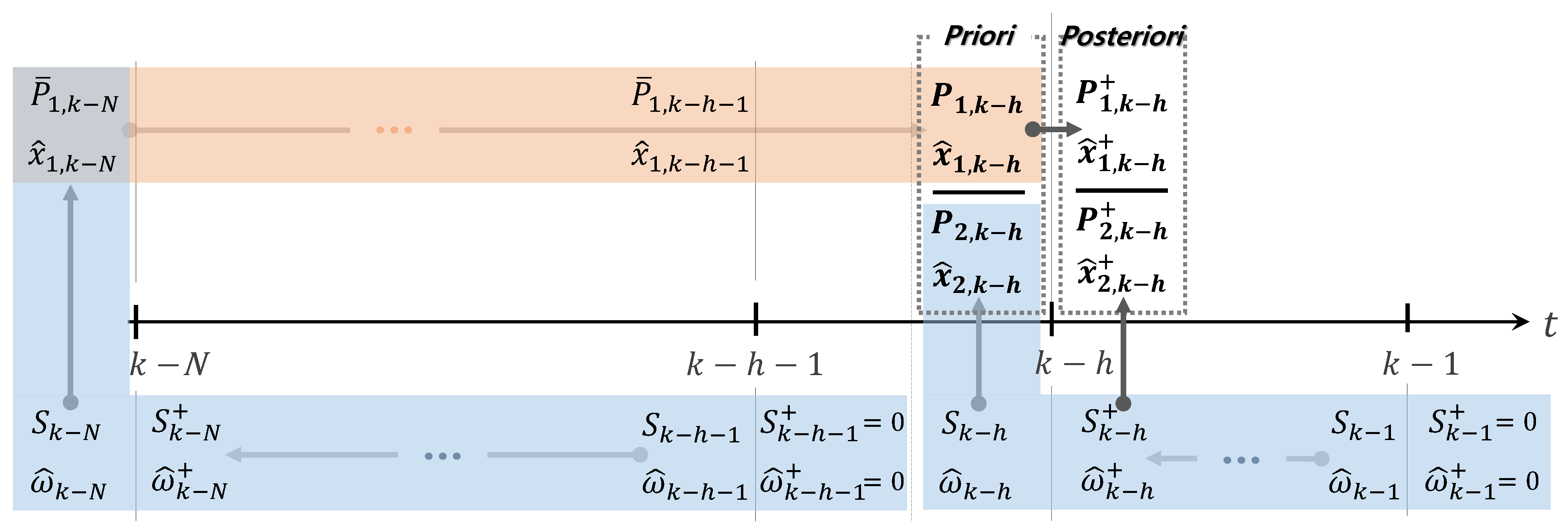
The overview of the proposed RUMVRHF smoother is shown in Figure 1.

Algorithm 1 Recursion of UMVRHF smoother on the horizon $[k-Nk-1]$.

Sub-horizon $[\mathit{k}-\mathit{N}\mathit{k}-\mathit{h}-\mathit{1}]$: 1: Initialization: $S_{k-h-1}^{+}\leftarrow 0$ and ${\widehat{w}}_{k-h1\mid k-h-1}^{+}\leftarrow 0$ 2: for $l\leftarrow 1$ to $N-h$ do $$\begin{array}{cc}\hfill S_{k-h-l}\leftarrow & C_{k-h-l}^T{R}_{k-h-l}^{-1}{C}_{k-h-l}+S_{k-h-l}^{+}\hfill \\ \hfill S_{k-h-l-1}^{+}\leftarrow & A_{k-h-l-1}^T{S}_{k-h-l}{A}_{k-h-l-1}-A_{k-h-l-1}^T{S}_{k-h-l}\hfill \\ & \hfill \times G_{k-h-l}{\left(Q_{k-h-l}^{-1}+G_{k-h-l}^T{S}_{k-h-l}{G}_{k-h-l}\right)}^{-1}\\ & \times G_{k-h-l}^T{S}_{k-h-l}{A}_{k-h-l-1}\hfill \\ \hfill {\widehat{w}}_{k-h-l\mid k-h-1}\leftarrow & C_{k-h-l}^T{R}_{k-h-l}^{-1}{y}_{k-h-l}+{\widehat{w}}_{k-h-l\mid k-h-1}^{+}\hfill \\ \hfill {\widehat{w}}_{k-h-l-1\mid k-h-1}^{+}\leftarrow & A_{k-h-l-1}^T{\widehat{w}}_{k-h-l\mid k-h-1}-A_{k-h-l-1}^T{S}_{k-h-l}\hfill \\ & \times G_{k-h-l}{\left(Q_{k-h-l}^{-1}+G_{k-h-l}^T{S}_{k-h-l}{G}_{k-h-l}\right)}^{-1}\hfill \\ & \times G_{k-h-l}^T{\widehat{w}}_{k-h-l\mid k-h-1}\hfill \end{array}$$ 3: end for 4: ${\widehat{x}}_{1,k-N\mid k-1}\leftarrow S_{k-N}^{-1}{\widehat{w}}_{k-N\mid k-h-1}$ and ${\overline{P}}_{1,k-N}\leftarrow S_{k-N}^{-1}$ 5: for $i\leftarrow 0$ to $N-h-1$ do $$\begin{array}{cc}\hfill {\widehat{x}}_{1,k-N+i+1\mid k-1}\leftarrow & A_{k-N+i}{\widehat{x}}_{1,k-N+i\mid k-1}-A_{k-N+i}{\overline{P}}_{1,k-N+i}{C}_{k-N+i}^T\hfill \\ & \times {\left(C_{k-N+i}{\overline{P}}_{1,k-N+i}{C}_{k-N+i}^T+R_{k-N+i}\right)}^{-1}\hfill \\ & \times \left(y_{k-N+i}-C_{k-N+i}{\widehat{x}}_{1,k-N+i\mid k-1}\right)\hfill \\ \hfill {\overline{P}}_{1,k-N+i+1}\leftarrow & A_{k-N+i}{\overline{P}}_{1,k-N+i}{A}_{k-N+i}^T-A_{k-N+i}{\overline{P}}_{1,k-N+i}{C}_{k-N+i}^T\hfill \\ & \times {\left(C_{k-N+i}{\overline{P}}_{1,k-N+i}{C}_{k-N+i}^T+R_{k-N+i}\right)}^{-1}{C}_{k-N+i}\hfill \\ & \times {\overline{P}}_{1,k-N+i}{A}_{k-N+i}^T+G_{k-N+i}{Q}_{k-N+i}{G}_{k-N+i}^T\hfill \end{array}$$ 6: end for 7: Initialization: $S_{k-1}^{+}\leftarrow 0$ and ${\widehat{w}}_{k-1\mid k-1}^{+}\leftarrow 0$ 8: for $l\leftarrow 1$ to h do $$\begin{array}{cc}\hfill S_{k-l}\leftarrow & C_{k-l}^T{R}_{k-l}^{-1}{C}_{k-l}+S_{k-l}^{+}\hfill \\ \hfill S_{k-l-1}^{+}\leftarrow & A_{k-l-1}^T{S}_{k-l}{A}_{k-l-1}-A_{k-l-1}^T{S}_{k-l}{G}_{k-l}(Q_{k-l}^{-1}\hfill \\ & +G_{k-l}^T{S}_{k-l}{G}_{k-l}{)}^{-1}{G}_{k-l}^T{S}_{k-l}{A}_{k-l-1},\hfill \\ \hfill {\widehat{w}}_{k-l\mid k-1}\leftarrow & C_{k-l}^T{R}_{k-l}^{-1}{y}_{k-l}+{\widehat{w}}_{k-l\mid k-1}^{+}\hfill \\ \hfill {\widehat{w}}_{k-l-1\mid k-1}^{+}\leftarrow & A_{k-l-1}^T{\widehat{w}}_{k-l\mid k-1}-A_{k-l-1}^T{S}_{k-l}{G}_{k-l}(Q_{k-l}^{-1}\hfill \\ & +G_{k-l}^T{S}_{k-l}{G}_{k-l}{)}^{-1}{G}_{k-l}^T{\widehat{w}}_{k-l\mid k-1}\hfill \end{array}$$ 9: end for 10: ${\widehat{x}}_{2,k-h\mid k-1}\leftarrow S_{k-h}^{-1}{\widehat{w}}_{k-h\mid k-1}$ and $P_{2,k-h}\leftarrow S_{k-h}^{-1}$ 10: Overall horizon $[\mathit{k}-\mathit{h}\mathit{k}-\mathit{1}]$ (optimal smoothed estimate): 11: $U_{1,k-h}\leftarrow P_{2,k-h}{\left(P_{1,k-h}+P_{2,k-h}\right)}^{-1}$ and $U_{2,k-h}\leftarrow P_{1,k-h}{\left(P_{1,k-h}+P_{2,k-h}\right)}^{-1}$ 12: ${\widehat{x}}_{k-h\mid k-1}\leftarrow U_{1,k-h}{\widehat{x}}_{1,k-h\mid k-1}+U_{2,k-h}{\widehat{x}}_{2,k-h\mid k-1}$ and $P_{k-h}\leftarrow {\left(P_{1,k-h}^{-1}+P_{2,k-h}^{-1}\right)}^{-1}$

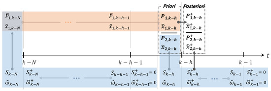
Figure 1. Concept and timing diagram of the RUMVRHF smoother.

4. Extensions of RUMVRHF Smoother

In this section, we introduce a method for extending the proposed RUMVRHF smoother to a posteriori state estimation. In addition, additional RHF smoothers are proposed based on the Rauch–Tung–Striebel smoothing algorithm and computational complexity reduction strategy.

4.1. Extension to Posteriori State Estimation

We first introduce an approach for extending the proposed recursive algorithm to a posteriori state estimation. By denoting the a posteriori estimates for the overall horizon $[k-Nk]$, sub-horizon $[k-Nk-h]$ and separated sub-horizon $[k-h+1k]$ as ${\widehat{x}}_{k-h\mid k}$, ${\widehat{x}}_{1,k-h\mid k}^{+}$ and ${\widehat{x}}_{2,k-h\mid k}^{+}$, respectively, the a posteriori overall estimate and its error covariance at time $k-h$ can be represented as follows [1]:

$$\begin{array}{ccc}\hfill {\widehat{x}}_{k-h\mid k}^{+}& =& U_{p1,k-h}{\widehat{x}}_{1,k-h\mid k}^{+}+U_{p2,k-h}{\widehat{x}}_{2,k-h\mid k}^{+},\hfill \end{array}$$

(87)

$$\begin{array}{ccc}\hfill P_{k-h}^{+}& =& {\left\{{\left(P_{1,k-h}^{+}\right)}^{-1}+{\left(P_{2,k-h}^{+}\right)}^{-1}\right\}}^{-1}\hfill \end{array}$$

(88)

where $P_{1,k-h}^{+}$ and $P_{2,k-h}^{+}$ are denoted as the state error covariance matrices of the estimates ${\widehat{x}}_{1,k-h\mid k}^{+}$ and ${\widehat{x}}_{2,k-h\mid k}^{+}$, respectively, and $U_{p1,k-h}$ and $U_{p2,k-h}$ are obtained from

$$\begin{array}{ccc}\hfill U_{p1,k-h}& =& P_{2,k-h}^{+}{\left(P_{1,k-h}^{+}+P_{2,k-h}^{+}\right)}^{-1},\hfill \end{array}$$

(89)

$$\begin{array}{ccc}\hfill U_{p2,k-h}& =& P_{1,k-h}^{+}{\left(P_{1,k-h}^{+}+P_{2,k-h}^{+}\right)}^{-1}.\hfill \end{array}$$

(90)

For the sub-horizon $[k-Nk-h]$, the a posteriori local estimate ${\widehat{x}}_{1,k-h\mid k}^{+}$ and its error covariance matrix $P_{1,k-h}^{+}$ can be updated from the predicted local estimates ${\widehat{x}}_{1,k-h\mid k}$ and its error covariance matrix $P_{1,k-h}$ as [1]

$$\begin{array}{ccc}\hfill {\widehat{x}}_{1,k-h\mid k}^{+}& =& {\widehat{x}}_{1,k-h\mid k}+P_{1,k-h}{C}_{k-h}^T{\left(C_{k-h}{P}_{1,k-h}{C}_{k-h}^T+R_{k-h}\right)}^{-1}\hfill \\ & & \times \left(y_{k-h}-C_{k-h}{\widehat{x}}_{1,k-h\mid k}\right),\hfill \end{array}$$

(91)

$$\begin{array}{ccc}\hfill P_{1,k-h}^{+}& =& P_{1,k-h}-P_{1,k-h}{C}_{k-h}^T{\left(C_{k-h}{P}_{1,k-h}{C}_{k-h}^T+R_{k-h}\right)}^{-1}{C}_{k-h}{P}_{1,k-h},\hfill \end{array}$$

(92)

respectively.

Because the recursive equations in Theorem 2 are equivalent to the conventional information filter formulation in [1], the posteriori information estimate ${\widehat{w}}_{k-h\mid k}^{+}$ and its posteriori information matrix $S_{k-h}^{+}$ can be obtained as ${\widehat{w}}_{k-h\mid k}^{+}={\left(P_{2,k-h}^{+}\right)}^{-1}{\widehat{x}}_{2,k-h\mid k}^{+}$ and $S_{k-h}^{+}={\left(P_{2,k-h}^{+}\right)}^{-1}$, respectively. Thus, the a posteriori local estimate ${\widehat{x}}_{2,k-h\mid k}^{+}$ and its error covariance matrix $P_{2,k-h}^{+}$ can be computed from the predicted ${\widehat{w}}_{k-h\mid k}^{+}$ and $S_{k-h}^{+}$ as follows:

$$\begin{array}{ccc}\hfill {\widehat{x}}_{2,k-h\mid k}^{+}& =& P_{2,k-h}^{+}{\widehat{w}}_{k-h\mid k}^{+}={\left(S_{k-h}^{+}\right)}^{-1}{\widehat{w}}_{k-h\mid k}^{+},\hfill \end{array}$$

(93)

$$\begin{array}{ccc}\hfill P_{2,k-h}^{+}& =& {\left(S_{k-h}^{+}\right)}^{-1},\hfill \end{array}$$

(94)

where $S_{k-h}^{+}$ and ${\widehat{w}}_{k-h\mid k}^{+}$ are calculated from (83) and (84) with boundary conditions $S_k^{+}=0$ and ${\widehat{w}}_{k\mid k}^{+}=0$.

4.2. Extension to Receding-Horizon Rauch-Tung-Striebel Fixed-Lag Smoother

Because the proposed RUMVRHF smoother is established based on two local optimal estimators, three steps are required to obtain the overall estimate and its error covariance matrix. Using the Rauch–Tung–Striebel (RTS) smoothing algorithm [25,26], the proposed recursive smoothing process can be implemented in two steps: filtering for the current state and smoothing for the fixed-lag state estimations. Although the estimation structure of RTS smoothing is different from that of the proposed smoother, it can provide computational efficiency and reliable results [27]. Thus, in this subsection, we propose a receding-horizon Rauch–Tung–Striebel fixed-lag (RHRTSF) smoother as an extension and application of the proposed recursive method.

First, the backward recursion of the overall posteriori covariance matrix $P_{k-l}^{+}$ on the time-interval $[k-hk]$ can be represented in terms of posteriori local covariance matrices ${\overline{P}}_{1,k-l}^{+}$ and $P_{2,k-l}^{+}$ as follows:

$$\begin{array}{ccc}\hfill P_{k-l}^{+}& =& {\overline{P}}_{1,k-l}^{+}-{\overline{P}}_{1,k-l}^{+}{\left({\overline{P}}_{1,k-l}^{+}+P_{2,k-l}^{+}\right)}^{-1}{\overline{P}}_{1,k-l}^{+}\hfill \\ & =& {\overline{P}}_{1,k-l}^{+}-{\overline{P}}_{1,k-l}^{+}{A}_{k-l+1}^T{\left({\overline{P}}_{1,k-l+1}+P_{2,k-l+1}\right)}^{-1}{A}_{k-l+1}{\overline{P}}_{1,k-l}^{+}\hfill \\ & =& {\overline{P}}_{1,k-l}^{+}-{\overline{P}}_{1,k-l}^{+}{A}_{k-l+1}^T[{\overline{P}}_{1,k-l+1}+\{{\left(P_{2,k-l+1}^{+}\right)}^{-1}+{\left({\overline{P}}_{1,k-l+1}^{+}\right)}^{-1}\hfill \\ & & -{\overline{P}}_{1,k-l+1}^{-1}{\}}^{-1}{]}^{-1}{A}_{k-l+1}{\overline{P}}_{1,k-l}^{+}\hfill \\ & =& {\overline{P}}_{1,k-l}^{+}-{\overline{P}}_{1,k-l}^{+}{A}_{k-l+1}^T{\left[{\overline{P}}_{1,k-l+1}+{\left\{{\left(P_{k-l+1}^{+}\right)}^{-1}-{\overline{P}}_{1,k-l+1}^{-1}\right\}}^{-1}\right]}^{-1}\hfill \\ & & \times A_{k-l+1}{\overline{P}}_{1,k-l}^{+}\hfill \\ & =& {\overline{P}}_{1,k-l}^{+}-{\overline{P}}_{1,k-l}^{+}{A}_{k-l+1}^T{\overline{P}}_{1,k-l+1}^{-1}[{\overline{P}}_{1,k-l+1}^{-1}+{\overline{P}}_{1,k-l+1}^{-1}\{{\left(P_{k-l+1}^{+}\right)}^{-1}\hfill \\ & & -{\overline{P}}_{1,k-l+1}^{-1}{\}}^{-1}{\overline{P}}_{1,k-l+1}^{-1}{]}^{-1}{A}_{k-l+1}{\overline{P}}_{1,k-l}^{+}\hfill \\ & =& {\overline{P}}_{1,k-l}^{+}-K_{k-l}\left({\overline{P}}_{1,k-l+1}-P_{k-l+1}^{+}\right)K_{k-l}^T,\hfill \end{array}$$

(95)

for $1\le l\le h$, where $K_{k-l}={\overline{P}}_{1,k-l}^{+}{A}_{k-l+1}^T{\overline{P}}_{1,k-l+1}^{-1}$.

Involving the same derivation as (95), the backward recursion of the overall smoothed estimates can be written as follows:

$$\begin{array}{ccc}\hfill {\widehat{x}}_{k-l\mid k}^{+}& =& {\widehat{x}}_{1,k-l\mid k}^{+}+K_{k-l}\left({\widehat{x}}_{k-l+1\mid k}^{+}-{\widehat{x}}_{1,k-l\mid k}\right),\hfill \end{array}$$

(96)

for $1\le l\le h$.

Thus, the RHRTSF smoother can be obtained by combining the receding horizon optimal filter on the overall horizon $[k-Nk]$ and backward recursions (95) and (96) by the following algorithm:

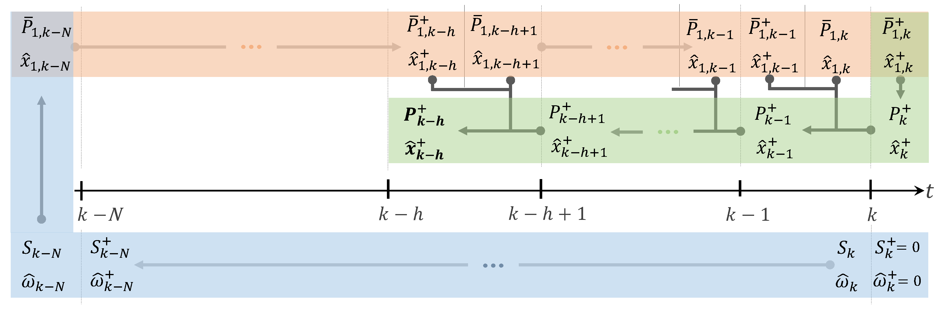
The concept of the proposed RHRTSF smoother is depicted in Figure 2.

Figure 2. Concept of the RHRTSF smoother.

4.3. Extension to Reduced Computational Complexity Receding Horizon Fixed-Lag Smoother

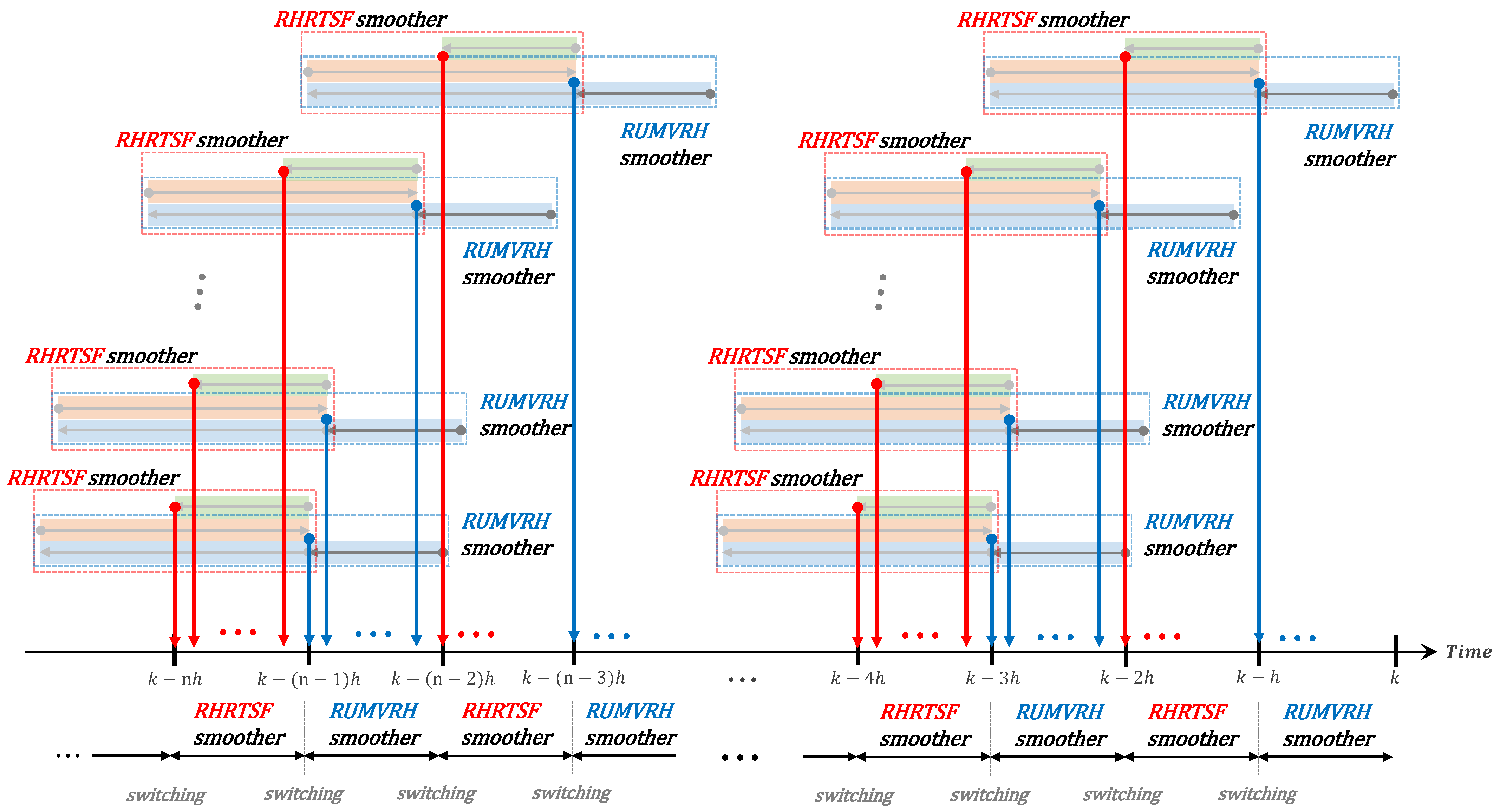
Although the proposed RUMVRHF and RTSRHF smoothers can provide more computational efficiency than RH smoothers in batch form, the computational complexity can be further improved by combining and sharing their estimates. In this section, we proposed the reduced computational complexity RHF (RCCRHF) smoother that periodically switches between RTSRHF and RUMVRHF smoothers to reduce the computational complexity of the proposed recursive smoothing algorithms.

The concept of RCCRHF smoothing algorithm is shown in Figure 3. As can be seen in the figure, the basic concept of the RCCRHF smoothing algorithm is a periodical switching RTSRHF and RUMVRHF smoothing algorithms and sharing their estimates.

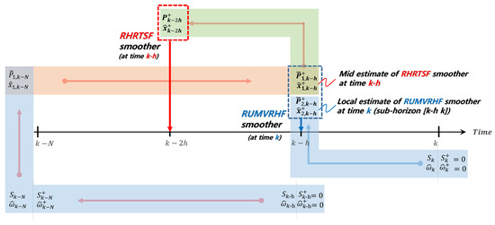
Figure 3. The concept of RCCRHF smoothing.

To illustrate the proposed RCCRHF smoothing algorithm, let us suppose that the RTSRHF smoother is selected at time $k-h$ and it estimates the lag state $x_{k-2h}$ by using measurements in the horizon $[k-Nk-h]$. The RCCRHF smoothing algorithm is started from the RTSRHF smoother. The horizon initial state ${\widehat{x}}_{1,k-N\mid k-h}^{+}$ and its error covariance $P_{1,k-N}^{+}$ are estimated through steps 1–4 of Algorithm 2. If we define the mid estimate and its error covariance as ${\widehat{x}}_{k-h\mid k-h}^{+\ast }={\widehat{x}}_{1,k-h\mid k-h}^{+}$ and ${\overline{P}}_{k-h}^{+\ast }=P_{1,k-h}^{+}$, respectively, these are obtained through the steps 5–9 in Algorithm 2. Thereafter, the final estimate ${\widehat{x}}_{k-2h\mid k-h}^{+}$ and its error covariance $P_{k-2h}^{+}$ are finally obtained through the steps 10–13 in Algorithm 2), with boundary conditions ${\widehat{x}}_{k-h\mid k-h}^{+\ast }$ and ${\overline{P}}_{k-h}^{+\ast }$. It is noted that this process is exactly same as the RHRTS smoothing algorithm except that the overall horizon length is taken as $N-h$, not N. Moreover, it is also noted that the mid estimate ${\widehat{x}}_{k-h\mid k-h}^{+\ast }$ and its error covariance ${\overline{P}}_{k-h}^{+\ast }$ are the same as the estimation results of minimum variance RH (MVRH) filter for the horizon $[k-Nk-h]$.

Now, suppose that the smoothing mode is changed to RUMVRHF smoother at time k and it estimates the lag state $x_{k-h}$ by using measurements on the horizon $[k-Nk]$. In the RUMVRHF smoothing process, the local estimate ${\widehat{x}}_{1,k-h\mid k}^{+}$ and its error covariance $P_{1,k-h}^{+}$ for the sub-horizon $[k-Nk-h]$ should be obtained through the MVRH filter. This estimation process is equivalent to obtain the mid estimate and its error covariance of RTSRHF smoother. This means that the mid estimate and its error covariance of RTSRHF smoother at time $k-h$ can be used as the local estimate and error covariance of RUMVRHF smoother at time k for the sub-horizon $[k-Nk-h]$, i.e., ${\widehat{x}}_{1,k-h\mid k}^{+}={\widehat{x}}_{k-h\mid k-h}^{+\ast }$ and $P_{1,k-h}^{+}=P_{k-h}^{+\ast }$, respectively. Thus, the overall smoothed estimate ${\widehat{x}}_{k-h\mid k}^{+}$ and its error covariance $P_{k-h}^{+}$ of RUMVRHF smoother are obtained as follows:

$$\begin{array}{ccc}\hfill {\widehat{x}}_{k-h\mid k}^{+}& =& U_{p1,k-h}{\widehat{x}}_{k-h\mid k-h}^{+\ast }+U_{p2,k-h}{\widehat{x}}_{2,k-h\mid k}^{+},\hfill \end{array}$$

(97)

$$\begin{array}{ccc}\hfill P_{k-h}^{+}& =& {\left\{{\left(P_{k-h}^{+\ast }\right)}^{-1}+{\left(P_{2,k-h}^{+}\right)}^{-1}\right\}}^{-1},\hfill \end{array}$$

(98)

$$\begin{array}{ccc}\hfill U_{p1,k-h}& =& P_{2,k-h}^{+}{\left(P_{k-h}^{+\ast }+P_{2,k-h}^{+}\right)}^{-1},\hfill \end{array}$$

(99)

$$\begin{array}{ccc}\hfill U_{p2,k-h}& =& P_{k-h}^{+\ast }{\left(P_{k-h}^{+\ast }+P_{2,k-h}^{+}\right)}^{-1},\hfill \end{array}$$

(100)

where ${\widehat{x}}_{2,k-h\mid k}^{+}$ and $P_{2,k-h}^{+}$ are the local estimate and its error covariance matrix for the sub-horizon $[k-hk]$, respectively, and ${\widehat{x}}_{k-h\mid k-h}^{+\ast }$ and $P_{k-h}^{\ast +}$ are obtained from the RTSRHF smoother on the overall horizon $[k-N-hk-h]$, not $[k-Nk-h]$.

Algorithm 2 RHRTSF smoothing algorithm on the horizon $[k-Nk]$.

Finite horizon Kalman filtering with estimated initial state 1: Initialization: $S_k^{+}\leftarrow 0$ and ${\widehat{w}}_{k\mid k}^{+}\leftarrow 0$ 2: for $l\leftarrow 0$ to N do $$\begin{array}{cc}\hfill S_{k-l}\leftarrow & C_{k-l}^T{R}_{k-l}^{-1}{C}_{k-l}+S_{k-l}^{+}\hfill \\ \hfill S_{k-l-1}^{+}\leftarrow & A_{k-l-1}^T{S}_{k-l}{A}_{k-l-1}-A_{k-l-1}^T{S}_{k-l}{G}_{k-l}\hfill \\ & \times {\left(Q_{k-l}^{-1}+G_{k-l}^T{S}_{k-l}{G}_{k-l}\right)}^{-1}{G}_{k-l}^T{S}_{k-l}{A}_{k-l-1}\hfill \\ \hfill {\widehat{w}}_{k-l\mid k}\leftarrow & C_{k-l}^T{R}_{k-l}^{-1}{y}_{k-l}+{\widehat{w}}_{k-l\mid k}^{+}\hfill \\ \hfill {\widehat{w}}_{k-l-1\mid k}^{+}\leftarrow & A_{k-l-1}^T{\widehat{w}}_{k-l\mid k}-A_{k-l-1}^T{S}_{k-l}{G}_{k-l}\hfill \\ & \times {\left(Q_{k-l}^{-1}+G_{k-l}^T{S}_{k-l}{G}_{k-l}\right)}^{-1}{G}_{k-l}^T{\widehat{w}}_{k-l\mid k}\hfill \end{array}$$ 3: end for 4: ${\widehat{x}}_{1,k-N\mid k}\leftarrow S_{k-N}^{-1}{\widehat{w}}_{k-N\mid k}$ and ${\overline{P}}_{1,k-N}\leftarrow S_{k-N}^{-1}$ 5: for $i\leftarrow 0$ to $N-h-2$ do $$\begin{array}{cc}\hfill {\widehat{x}}_{1,k-N+i+1\mid k}\leftarrow & A_{k-N+i}{\widehat{x}}_{1,k-N+i\mid k-1}-A_{k-N+i}{\overline{P}}_{1,k-N+i}{C}_{k-N+i}^T\hfill \\ & \times {\left(C_{k-N+i}{\overline{P}}_{1,k-N+i}{C}_{k-N+i}^T+R_{k-N+i}\right)}^{-1}\hfill \\ & \times \left(y_{k-N+i}-C_{k-N+i}{\widehat{x}}_{1,k-N+i\mid k-1}\right)\hfill \\ \hfill {\overline{P}}_{1,k-N+i+1}\leftarrow & A_{k-N+i}{\overline{P}}_{1,k-N+i}{A}_{k-N+i}^T-A_{k-N+i}{\overline{P}}_{1,k-N+i}{C}_{k-N+i}^T\hfill \\ & \times {\left(C_{k-N+i}{\overline{P}}_{1,k-N+i}{C}_{k-N+i}^T+R_{k-N+i}\right)}^{-1}{C}_{k-N+i}\hfill \\ & \times {\overline{P}}_{1,k-N+i}{A}_{k-N+i}^T+G_{k-N+i}{Q}_{k-N+i}{G}_{k-N+i}^T\hfill \end{array}$$ 6: end for 7: $$\begin{array}{cc}\hfill {\widehat{x}}_{1,k-h-1\mid k}^{+}\leftarrow & {\widehat{x}}_{1,k-h-1\mid k}+P_{1,k-h-1}{C}_{k-h-1}^T(C_{k-h-1}{P}_{1,k-h-1}{C}_{k-h-1}^T\hfill \\ & +R_{k-h-1}{)}^{-1}\left(y_{k-h-1}-C_{k-h-1}{\widehat{x}}_{1,k-h-1\mid k}\right),\hfill \\ \hfill P_{1,k-h-1}^{+}\leftarrow & P_{1,k-h-1}-P_{1,k-h-1}{C}_{k-h-1}^T(C_{k-h-1}{P}_{1,k-h-1}{C}_{k-h-1}^T\hfill \\ & +R_{k-h-1}{)}^{-1}{C}_{k-h-1}{P}_{1,k-h-1},\hfill \end{array}$$ 8: for $i\leftarrow 0$ to h do $$\begin{array}{cc}\hfill {\widehat{x}}_{1,k-h+i\mid k}\leftarrow & A_{k-h+i}{\widehat{x}}_{1,k-h+i-1\mid k}^{+}\hfill \\ \hfill {\overline{P}}_{1,k-h+i}\leftarrow & A_{k-h+i}{\overline{P}}_{1,k-h+i-1}^{+}{A}_{k-h+i}^T+G_{k-h+i}{Q}_{k-h+i}{G}_{k-h+i}^T\hfill \\ \hfill {\widehat{x}}_{1,k-h+i\mid k}^{+}\leftarrow & {\widehat{x}}_{1,k-h+i\mid k}+{\overline{P}}_{1,k-h+i}{C}_{k-h+i}^T(C_{k-h+i}{\overline{P}}_{1,k-h+i}{C}_{k-h+i}^T\hfill \\ & +R_{k-h+i}{)}^{-1}\left(y_{k-h+i}-C_{k-h+i}{\widehat{x}}_{1,k-h+i\mid k1}\right)\hfill \\ \hfill {\overline{P}}_{1,k-h+i}^{+}\leftarrow & {\overline{P}}_{1,k-h+i}-{\overline{P}}_{1,k-h+i}{C}_{k-h+i}^T(C_{k-h+i}{\overline{P}}_{1,k-h+i}{C}_{k-h+i}^T\hfill \\ & +R_{k-h+i}{)}^{-1}{C}_{k-h+i}{\overline{P}}_{1,k-h+i},\hfill \end{array}$$ 9: end for   Backward recursion: 10:     Initialization: $P_k^{+}\leftarrow {\overline{P}}_{1,k}^{+}$ and ${\widehat{x}}_{k\mid k}^{+}\leftarrow {\widehat{x}}_{1,k\mid k}^{+}$ 11:     for $l\leftarrow 1$ to h do $$\begin{array}{cc}\hfill K_{k-l}\leftarrow & {\overline{P}}_{1,k-l}^{+}{A}_{k-l+1}^T{\overline{P}}_{1,k-l+1}^{-1}\hfill \\ \hfill {\widehat{x}}_{k-l\mid k}^{+}\leftarrow & {\widehat{x}}_{1,k-l\mid k}^{+}+K_{k-l}\left({\widehat{x}}_{k-l+1\mid k}^{+}-{\widehat{x}}_{1,k-l\mid k}\right)\hfill \\ \hfill P_{k-l}^{+}\leftarrow & {\overline{P}}_{1,k-l}^{+}-K_{k-l}\left({\overline{P}}_{1,k-l+1}-P_{k-l+1}^{+}\right)K_{k-l}^T\hfill \end{array}$$ 12:     end for 13:     Return: ${\widehat{x}}_{k-h\mid k}^{+}$ and $P_{k-h}^{+}$

Therefore, RCCRHF smoother can be designed by switching the roles of RTSRHF and RUMVRHF smoothers in every h time step periodically. The concept of periodical switching scheme for RCCRHF smoother is depicted in Figure 4.

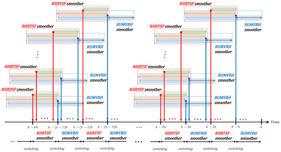
Figure 4. Concept of periodical swithcing scheme for RHCCRHF smoother.

The process for obtaining the local estimate and its error covariance of RUMVRHF smoother can be eliminated by sharing the mid estimate and its error covariance of RTSRHF smoother at the h lag time. Thus, the RCCRHF smoother could have less computation time than the proposed recursive RHF smoothers.

However, if the lag size h is greater than half of the horizon length $N-h$, the RSTRHF smoother cannot be defined. In this situation, the overall horizon lengths of the RSTRHF and RUMVRHF smoothers are taken as N and $N+h$, respectively. Although the horizon length of the RTSRHF smoother is increased by h, the RCCRHF smoother has less computation time of other proposed recursive RHF smoothers because $2N$ iterations to obtain local estimate and its covariance of RUMVRHF smoother is omitted.

5. Numerical Experiments and Discussion

In this section, numerical experimental results present the performance and effectiveness of the proposed RHF smoothing algorithms.

5.1. F-404 Gas Turbine Aircraft Engine System

We consider the following discrete time F-404 gas turbine aircraft engine model [21].

$$\begin{array}{ccc}\hfill x_{k+1}& =& \left[\begin{array}{ccc}0.9305+{\delta }_k& 0& 0.1107\\ 0.0077& 0.9802+{\delta }_k& -0.0173\\ 0.0142& 0& 0.8953+{\delta }_k\end{array}\right]x_k+\left[\begin{array}{c}1\\ 1\\ 1\end{array}\right]w_k,\hfill \end{array}$$

(101)

$$\begin{array}{ccc}\hfill y& =& \left[\begin{array}{ccc}1+0.1{\delta }_k& 0& 0\\ 0& 1+0.1{\delta }_k& 0\end{array}\right]x_k+v_k,\hfill \end{array}$$

(102)

where the initial state $x_0=[000{]}^T$, initial error covariance matrix $P_0={10}^3{I}_{3\times 3}$, and the actual process and measurement noise covariance matrices are considered as $Q=0.2^2$ and $R=0.{01}^2{I}_{2\times 2}$, respectively.

To demonstrate the robustness against temporary modeling uncertainty of the proposed smoothers upon the occurrence of a model mismatch, the model uncertain parameter ${\delta }_k$ is considered as follows:

$$\begin{array}{c}\hfill {\delta }_k=\left\{\begin{array}{cc}0.1,& 200\le k\le 250,\\ 0,& otherwise.\end{array}\right.\end{array}$$

Smoothers are designed for the nominal state space models (101) and (102), considering ${\delta }_k=0$; therefore, they are applied to the temporarily uncertain system. We set the process covariance and measurement noise covariance matrices for smoothers as $Q=0.{19}^2$ and $R=0.{018}^2{I}_{2\times 2}$, respectively. Because the estimates of the nominal FMS smoother, i.e., forgetting factor $\lambda =1$, diverge for the system model, the forgetting factor is considered as $\lambda =0.9$.

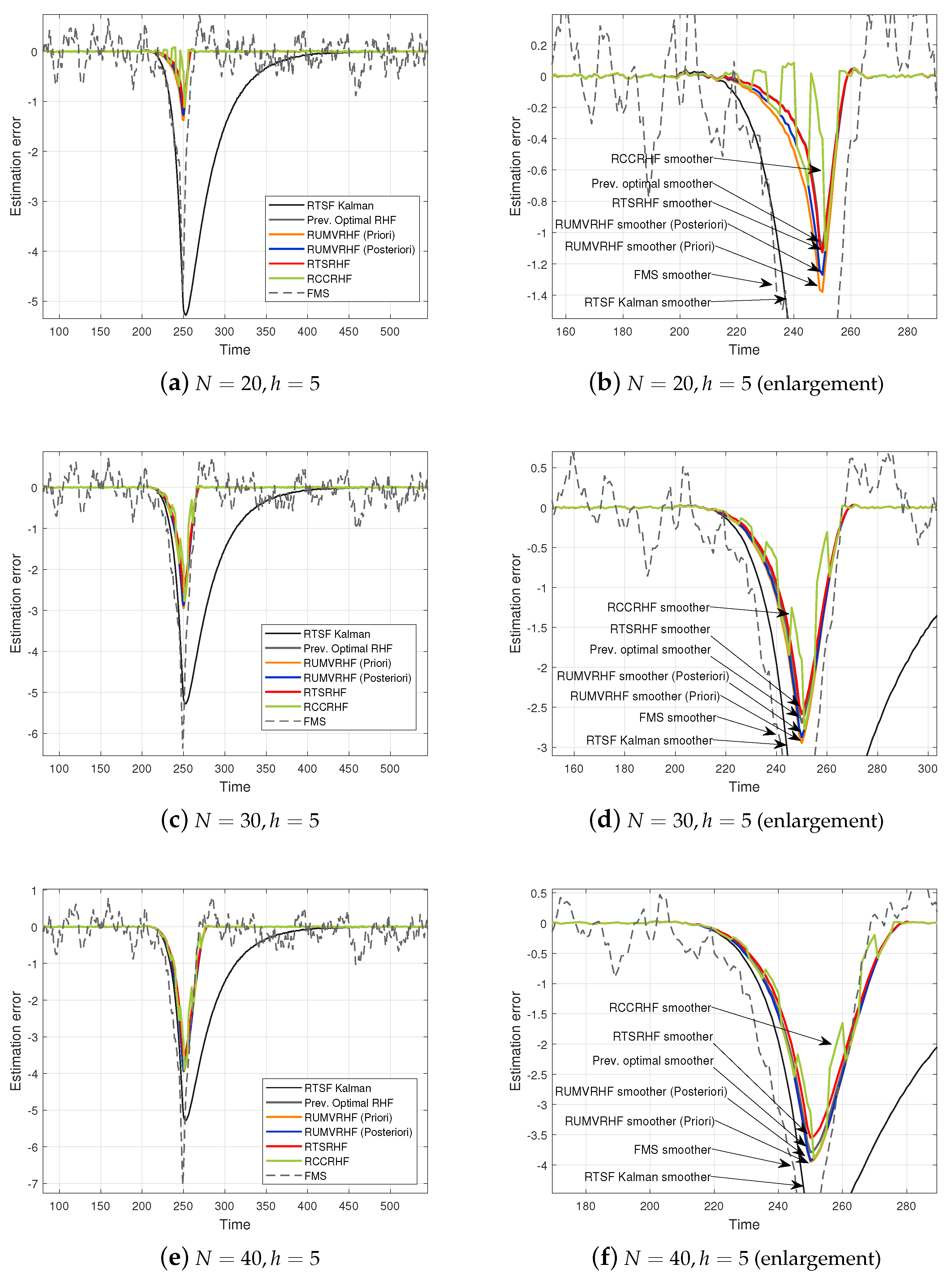
First, to verify the performance of the proposed algorithms, the proposed RHF smoothers are compared with the Rauch–Tung–Striebel fixed-lag (RTSF) Kalman [1], the previous optimal RHF [20], and the FMS smoothers [21]. The second state estimation errors and time averaged values of the root-mean square estimation (RMSE) errors are shown for various horizon lengths in Figure 5 and Table 1, Table 2 and Table 3, respectively.

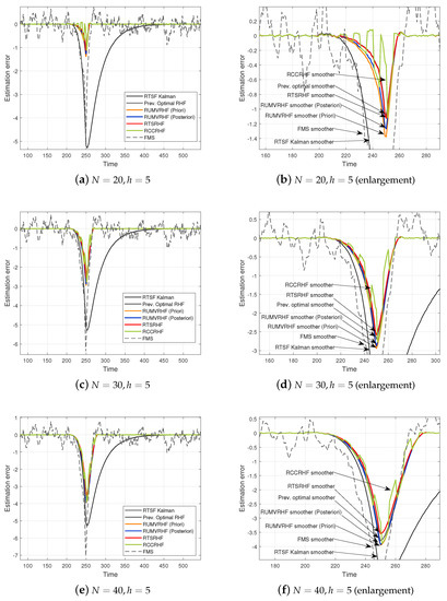
Figure 5. Estimation errors with respect to various horizon lengths ($h=5$).

Table 1. RMSE errors for the time interval $\left[50500\right]$.

Horizon Length and Lag Size	$\mathit{N}=20$, $\mathit{h}=5$	$\mathit{N}=30$, $\mathit{h}=5$	$\mathit{N}=40$, $\mathit{h}=5$
RTSF Kalman smoother	$1.386$	$1.386$	$1.386$
Prev. optimal RHF smoother	$0.135$	$0.437$	$0.709$
RUMVRHF smoother (Priori)	$0.186$	$0.482$	$0.740$
RUMVRHF smoother (Posteriori)	$0.166$	$0.469$	$0.735$
RTSRHF smoother	$0.140$	$0.417$	$0.661$
RCCRHF smoother	$\mathbf{0}.\mathbf{113}$	$\mathbf{0}.\mathbf{384}$	$\mathbf{0}.\mathbf{647}$
FMS smoother	$0.674$	$0.977$	$1.125$

Table 2. RMSE errors for the time interval $\left[50200\right]$$(\times {10}^{-3})$.

Horizon Length and Lag Size	$\mathit{N}=20$, $\mathit{h}=5$	$\mathit{N}=30$, $\mathit{h}=5$	$\mathit{N}=40$, $\mathit{h}=5$
RTSF Kalman smoother	$\mathbf{7}.\mathbf{386}$	$7.386$	$7.386$
Prev. optimal RHF smoother	$7.848$	$\mathbf{7}.\mathbf{321}$	$\mathbf{7}.\mathbf{341}$
RUMVRHF smoother (Priori)	$8.031$	$7.355$	$7.357$
RUMVRHF smoother (Posteriori)	$7.968$	$7.345$	$7.352$
RTSRHF smoother	$7.892$	$7.323$	$7.345$
RCCRHF smoother	$7.956$	$7.393$	$7.378$
FMS smoother	$324.983$	$342.122$	$343.178$

Table 3. RMSE errors for the time interval $\left[201350\right]$.

Horizon Length and Lag Size	$\mathit{N}=20$, $\mathit{h}=5$	$\mathit{N}=30$, $\mathit{h}=5$	$\mathit{N}=40$, $\mathit{h}=5$
RTSF Kalman smoother	$2.312$	$2.312$	$2.312$
Prev. optimal RHF smoother	$0.225$	$0.729$	$1.184$
RUMVRHF smoother (Priori)	$0.310$	$0.805$	$1.235$
RUMVRHF smoother (Posteriori)	$0.276$	$0.784$	$1.228$
RTSRHF smoother	$0.233$	$0.695$	$1.104$
RCCRHF smoother	$\mathbf{0}.\mathbf{189}$	$\mathbf{0}.\mathbf{642}$	$\mathbf{1}.\mathbf{080}$
FMS smoother	$1.051$	$15.677$	$1.817$

As observed in these results, the proposed RHF smoothers successfully estimate the real state and have better estimation performance than others. In comparison to the RTSF Kalman smoother, the RMSE errors of the proposed smoothers with small horizon lengths are a little bigger than that of the RTSF Kalman smoother when there are no modeling uncertainties.

However, in the case of large horizon lengths, the RMSE errors of the proposed smoothers are smaller than that of the RTSF Kalman smoother. Moreover, the estimation errors of the proposed RHF smoothers are remarkably smaller than that of the RTSF Kalman smoother for the cases of model mismatches. Furthermore, the estimated states of the proposed RHF smoothers rapidly converge to the real state after the modeling uncertainty disappears, whereas those of the RTSF Kalman smoother take a long time to converge. Hence, it can be deduced that the proposed RHF smoothers are more robust against temporary modeling uncertainty than the RTSF Kalman smoother.

In contrast to the previous optimal RHF smoother, the RMSE errors of the proposed RHF smoothers are slightly larger; however, they are similar to those of the previous optimal RHF smoother in the absence of modeling uncertainties. However, the estimation performance of the proposed RCCRHF and RTSRHF smoothers is better than that of the previous optimal RHF smoother when modeling uncertainties exist. Moreover, the estimation errors of the proposed RCCRHF and RTSRHF smoothers are getting smaller than that of the previous optimal RHF smoother, as well as increasing the horizon length of RHF smoothers. Furthermore, we can observe that the RMS errors of the RUMVRHF smoothers (a priori and a posteriori) are still slightly larger than those of the previous optimal RHF smoother, although the horizon length is increased.

By comparing the results for the RTSRHF and RUMVRHF smoothers, it can be stated that the estimation performance is affected, albeit not severely, by the information state, information matrix, and their initial conditions. Moreover, the structure of the RTSRHF smoother is better than that of the RUMVRHF smoother.

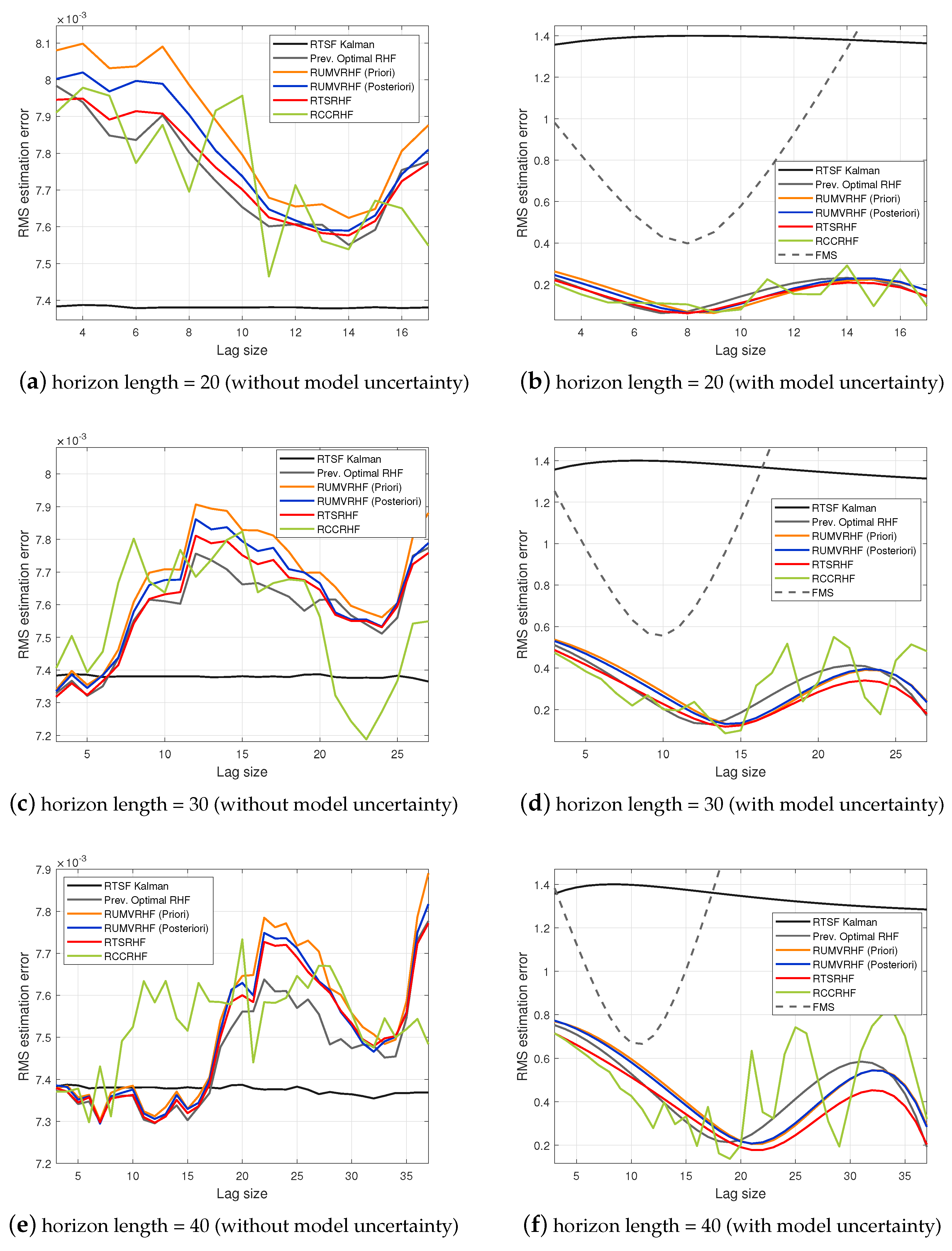
Second, to highlight the effects of the horizon length and delay size on the proposed RHF smoothers, we compare the RMSE errors of the smoothers with respect to various horizon lengths and lag sizes, as shown in Figure 6.

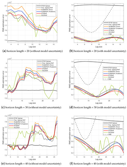
Figure 6. RMSE errors with respect to the various horizon lengths and lag sizes.

In contrast to all RMSE errors, it can be observed that the proposed RCCRHF and RTSRHF smoothers and the previous optimal RHF smoother can be optimal choices for short lag sizes. In particular, in Figure 6c,e, it can be observed that RHF smoothers with long horizon lengths and short delay sizes perform better than RTSF Kalman smoother, even in the absence of modeling uncertainties. In addition, the RHF smoothers with large horizon lengths yield better estimation results than those with small horizon lengths in the case of an accurate system model.

However, other proposed smoothers are also acceptable for use. From Figure 6b,d,f, it is observed that the proposed RCCRHF smoother with a short delay size provides better estimation performance than others in the case of a model mismatch because its averaged horizon length is shorter than other RHF smoothers. However, the RCCRHF smoother with a long delay size (longer than half of the horizon length) demonstrates poor estimation results owing to its increased horizon length. Thus, it can be stated, in the case of a model mismatch, a short lag size should be adopted for the proposed RCCRHF smoother.

As observed in Figure 6a,c,e, the estimation performance of the previous optimal RHF smoother is better than the other proposed RHF smoothers. On the contrary, observing the results in Figure 6b,d,f, it can easily noticed that the proposed smoothers demonstrate better estimation performance than the previous optimal RHF smoother except for small lag size intervals. In particular, the proposed RTSRHF smoother guarantees its estimation performance for most lag sizes. Thus, we can infer that the proposed smoothers are robust and provide more exact estimate than the previous optimal RHF smoother. Furthermore, we can observe that there is best lag size, and it is close to half of the horizon length.

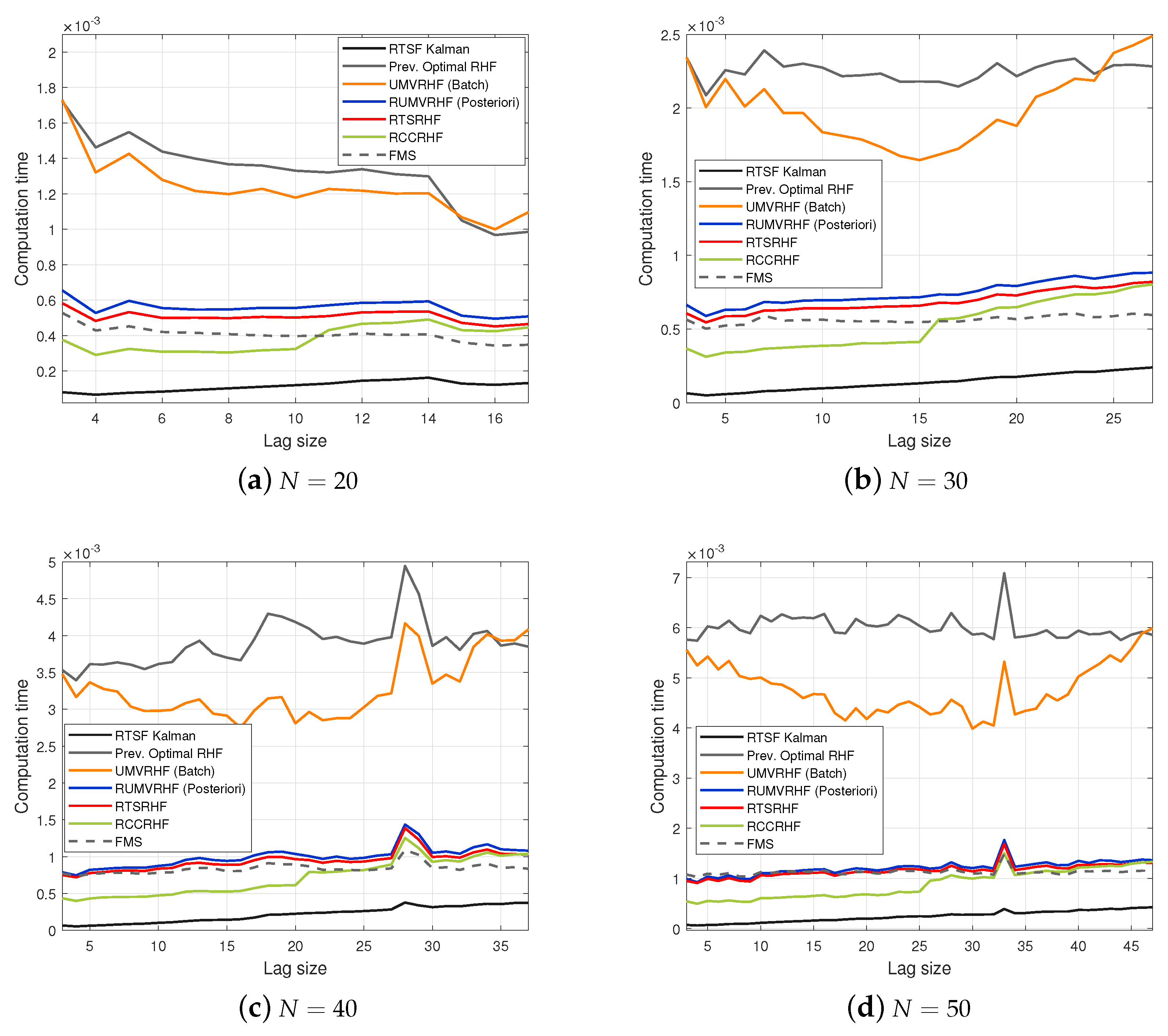
Third, to demonstrate the computational efficiency of the proposed approaches, the time-averaged computation times of RHF smoothers are compared, as presented in Table 4 and Figure 7. For fair comparisons, the matrix gains of the batch RHF smoothers are calculated at every iteration, although the smoothers are designed for time-invariant systems.

Table 4. Average computation time of RHF smoothers ($msec$).

Horizon Length and Lag Size	$\mathit{N}=20$, $\mathit{h}=5$	$\mathit{N}=30$, $\mathit{h}=5$	$\mathit{N}=40$, $\mathit{h}=5$	$\mathit{N}=50$, $\mathit{h}=5$
Prev. optimal RHF smoother	$1.548$	$2.257$	$3.611$	$6.026$
UMVRHF smoother (Batch)	$1.426$	$2.196$	$3.367$	$5.425$
RUMVRHF smoother (Posteriori)	$0.596$	$0.631$	$0.821$	$1.037$
RTSRHF smoother	$0.532$	$0.587$	$0.777$	$0.992$
RCCRHF smoother	$\mathbf{0}.\mathbf{325}$	$\mathbf{0}.\mathbf{341}$	$\mathbf{0}.\mathbf{458}$	$\mathbf{0}.\mathbf{552}$
FMS smoother	$0.452$	$0.523$	$0.764$	$1.095$

Figure 7. Time-averaged computation time with respect to the horizon lengths and lag sizes.

As observed from these results, the proposed UMVRHF smoothers in a separated batch-form have better computational performance than the previous optimal RHF smoothers in batch form. In Figure 7, we can observe that the computational efficiency of the proposed UMVRHF smoothers in a separated batch form can be improved by selecting the lag size near the half of the horizon length. Moreover, the proposed RHF smoothers in a recursive-form have much smaller computation times than RHF smoothers in a batch-form. It is clearly noticeable that the proposed RCCRHF smoothers involving short lag sizes (shorter than half of horizon length) have much smaller averaged computation times than other smoothers.

In addition, for a long lag size (larger than the half of the horizon length), the computation time is still smaller than that of the other proposed RHF smoothers, although their horizon sizes are longer than the others. Furthermore, the proposed RTSRHF smoothers have better computational performance than the proposed RUMVRHF smoothers.

5.2. Direct Current Motor System

In this subsection, numerical experiment results are given for direct current (DC) motor system to verify the applicability of the proposed methods for more practical application.

The discrete-time DC motor model with model uncertainty is given as follows [28,29]:

$$\begin{array}{ccc}\hfill x_{k+1}& =& \left[\begin{array}{cc}0.8178+{\delta }_k& -0.0011\\ 0.0563& 0.3678+{\delta }_k\end{array}\right]x_k+\left[\begin{array}{cc}0.0006& 0\\ 0& 0.0057\end{array}\right]w_k,\hfill \end{array}$$

(103)

$$\begin{array}{ccc}\hfill y_k& =& \left[\begin{array}{cc}1+0.1{\delta }_k& 0\end{array}\right]x_k+v_k,\hfill \end{array}$$

(104)

where the DC motor is assumed to be operated without any payload and drive voltage is assumed to be encountered as an external unit step source. Covariances for system and measurement noises are taken as $Q=0.{01}^{2}I$ and $R=0.{01}^2$, respectively, and the system parameters of DC motor system are shown in Table 5.

Table 5. Parameters of DC motor.

Description	Units	Value
Armature Current	A	state variable $\left(x_1\right)$
Rotational Speed	rad/s	state variable $\left(x_2\right)$
Armature Resistance	$\mathsf{\Omega }$	1
Armature Inductance	H	0.5
Motor Torque Constant	Nm/A	0.01
Motor Inertial Coefficient	Nm/(rad/s2)	0.01
Motor Viscous Friction Coefficient	Nm/(rad/s)	0.1

The model uncertain parameter ${\delta }_k$ for model mismatch is considered as

$$\begin{array}{c}\hfill {\delta }_k=\left\{\begin{array}{cc}0.05,& 200\le k\le 350,\\ 0,& otherwise.\end{array}\right.\end{array}$$

For RH smoothers, the horizon length and fixed-lag size are taken as $N=35$ and $h=3$, respectively. As shown in the previous experiment, the estimation performance of RUMVRHF smoother for posteriori priori state and batch form are similar to that of the RUMVRHF smoother for posteriori. Thus, in this section, we compare the estimation results of the RUMVRHF smoother (posteriori), RCCRHF smoother, RTSRHF smoother, FMS smoother, and RTSF Kalman smoother.

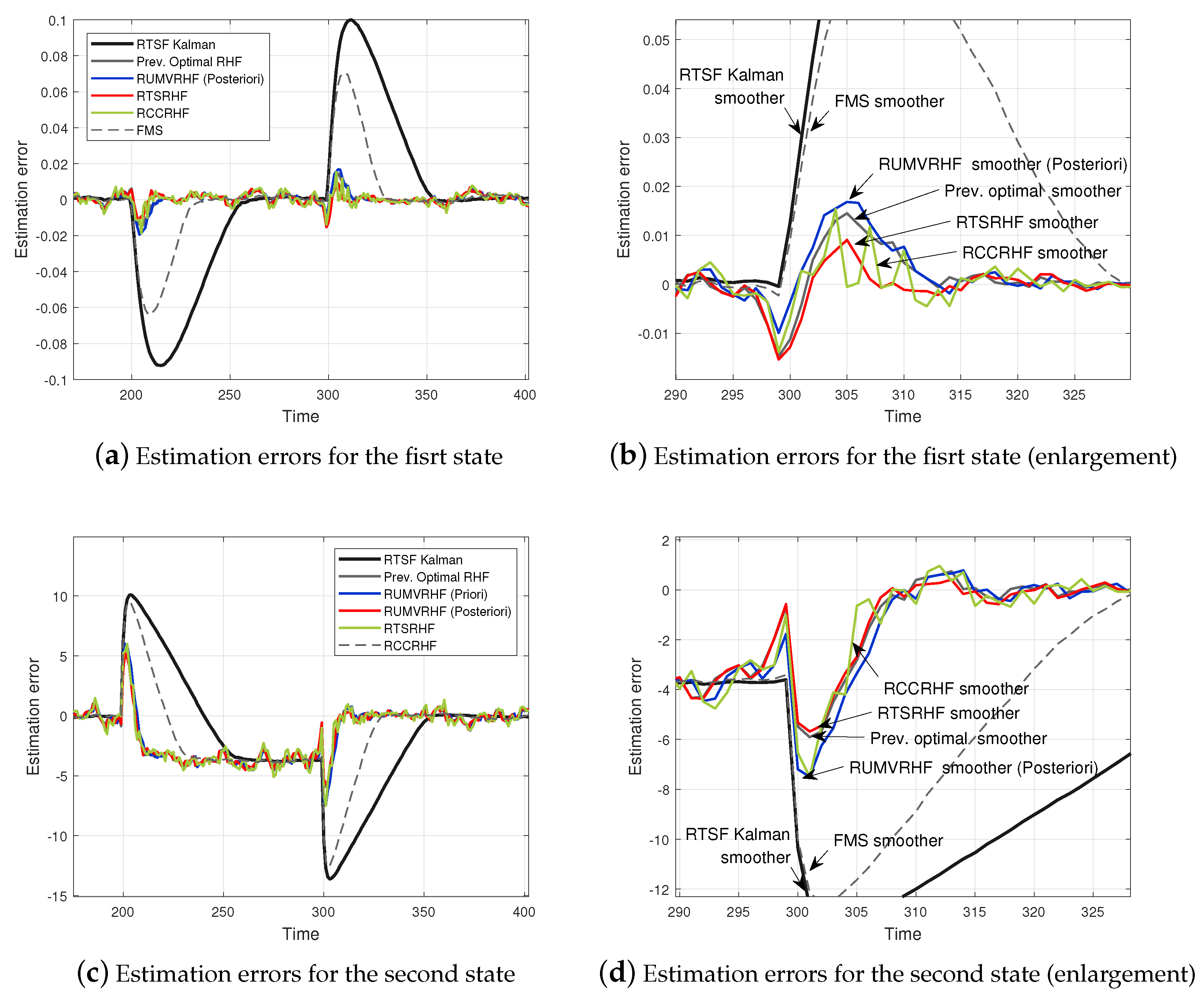
Figure 8 and Table 6 present estimation errors and time averaged values of RMSE errors of smoothers for $200\le k\le 350$. In addition, the average computation times of RHF smoothers are presented in Table 7.

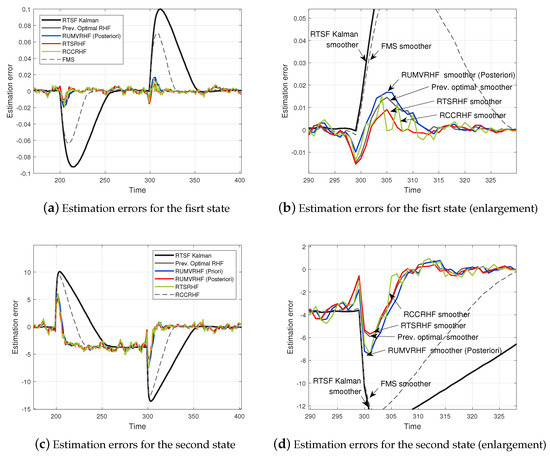
Figure 8. Estimation errors of smoothers.

Table 6. RMSE errors of smoothers for the time interval $\left[200350\right]$.

Smoothers	RMSE Error $\left({\mathit{x}}_1\right)$	RMSE Error $\left({\mathit{x}}_2\right)$
RTSF Kalman smoother	$0.0540$	$6.3353$
Prev. optimal RHF smoother	$0.0044$	$3.1536$
RUMVRHF smoother (Posteriori)	$0.0051$	$3.2190$
RTSRHF smoother	$\mathbf{0}.\mathbf{0034}$	$\mathbf{3}.\mathbf{0504}$
RCCRHF smoother	$0.0040$	$3.0770$
FMS smoother	$0.0282$	$4.8560$

Table 7. Average computation times of RHF smoothers.

Smoothers	Average Computation Time $\left(\mathit{m}\mathit{s}\mathit{e}\mathit{c}\right)$
Prev. optimal RHF smoother	$3.0829$
RUMVRHF smoother (Posteriori)	$1.1896$
RTSRHF smoother	$1.0909$
RCCRHF smoother	$\mathbf{0}.\mathbf{4852}$
FMS smoother	$0.6780$

As shown in these results, the proposed RHF smoothers estimate the real state well and provide more exact estimates than RTSF Kalman smoother for the modeling uncertainty. Moreover, the proposed RHF smoothers have faster convergence speed than RTSF Kalman smoother as we expected. Furthermore, the proposed RCCRHF smoother has better computational performance than other compared RHF smoothers. These observations show that the proposed RHF smoothers can work well and have robustness against temporarily modeling uncertainty for practical application.

6. Conclusions

In this paper, novel optimal RHF smoothers have been proposed in batch and recursive forms for linear discrete time-varying state space models. The proposed RHF smoothers were obtained by optimally combining local optimal receding horizon filters and smoothers for the separated sub-horizons. The proposed recursive RHF smoothing algorithm was formulated as a finite horizon Kalman filtering and information smoothing. Additionally, as an extension of the proposed recursive RHF smoothing algorithm, a Rauch–Tung–Striebel type RHF smoothing algorithm and reduced computational complexity RHF smoother were also proposed to improve the computational efficiency. The proposed RHF smoothers could provide optimality, unbiasedness, and bounded-input bounded-output stability. Moreover, the proposed RHF smoothers are independent of any a priori information of the initial state and assumption of a non-singular transition system matrix. Furthermore, the proposed RHF smoothers could significantly improve the computational efficiency, which is major disadvantage of RHF smoothers. Finally, it has been demonstrated via numerical experiments that the RHF smoothers proposed in this paper can provide better estimation results than fixed-lag Kalman smoothers in the case of a model mismatch. Furthermore, it was also shown that the proposed methods are more computational efficient than the existing RHF smoothers and applicable for practical application.

However, it is possible to improve the estimation perforamance of the RH smoothing algorithms by choosing the appropriate fixed lag size and horizon length. Thus, we plan to investigate the horizon length adjustment method and how to find optimal fixed-lag size for further improvement of the proposed RH smoothers as future work. Moreover, in the future, it would be meaningful to extend and evaluate the proposed RH smoothing algorithms for more practical applications.

References

- Lewis, F.L. Optimal Estimation: With An Introduction to Stochastic Control Theory; John Wiley and Sons: Hoboken, NJ, USA, 1986. [Google Scholar]
- Martino, L.; Read, J. A joint introduction to Gaussian Processes and Relevance Vector Machines with connections to Kalman filtering and other kernel smoothers. Inf. Fusion 2021, 74, 17–38. [Google Scholar] [CrossRef]
- Eilers, P.H.C.; Marx, B.D. Practical Smoothing: The Joys of P-Splines; Cambridge University Press: Cambridge, UK, 2021. [Google Scholar]
- Poddar, S.; Crassidis, J.L. Adaptive Lag Smoother for State Estimation. Sensors 2022, 22, 5310. [Google Scholar] [CrossRef] [PubMed]
- Lastre-Domínguez, C.; Ibarra-Manzano, O.; Andrade-Lucio, J.A.; Shmaliy, Y.S. Denoising ECG Signals Using Unbiased FIR Smoother and Harmonic State-Space Model. In Proceedings of the 28th European Signal Processing Conference (EUSIPCO), Amsterdam, The Netherlands, 18–21 January 2021; pp. 1279–1283. [Google Scholar]
- Si, Y. LPPCNN: A Laplacian Pyramid-based Pulse Coupled Neural Network Method for Medical Image Fusion. J. Appl. Sci. Eng. 2021, 24, 299–305. [Google Scholar]
- Ullah, I.; Qureshi, M.B.; Khan, U.; Memon, S.A.; Shi, Y.; Peng, D. Multisensor-Based Target-Tracking Algorithm with Out-of-Sequence-Measurements in Cluttered Environments. Sensors 2018, 18, 4043. [Google Scholar] [CrossRef] [PubMed]
- Tao, H.; Yanzhang, Z.; Hongxia, N.; Mingxi, C.; Shan, W. Research on Tracking Foreign Objects in Railway Tracks Based on Hidden Markov Kalman Filter. J. Appl. Sci. Eng. 2022, 25, 893–903. [Google Scholar]
- Kim, P.S. Finite Memory Structure Filtering and Smoothing for Target Tracking in Wireless Network Environments. Appl. Sci. 2019, 9, 2872. [Google Scholar] [CrossRef]
- Rau, J.C.; Wu, P.H.; Li, W.L. Test Slice Difference Technique for Low-Transition Test Data Compression. J. Appl. Sci. Eng. 2012, 15, 157–166. [Google Scholar]
- Lagerblad, U.; Wentzel, H.; Kulachenko, A. Dynamic response identification based on state estimation and operational modal analysis. Mech. Syst. Signal Process 2019, 129, 37–53. [Google Scholar] [CrossRef]
- Maes, K.; Gillijns, S.; Lombaert, G. A smoothing algorithm for joint input–state estimation in structural dynamics. Mech. Syst. Signal Process 2018, 98, 292–309. [Google Scholar] [CrossRef]
- Lagerblad, U.; Wentzel, H.; Kulachenko, A. Study of a fixed-lag Kalman smoother for input and state estimation in vibrating structures. Inverse Probl. Sci. Eng. 2021, 29, 1260–1281. [Google Scholar] [CrossRef]
- Vauhkonen, P.J.; Vauhkonen, M.; Kaipio, J.P. Fixed-lag smoothing and state estimation in dynamic electrical impedance tomography. Int. J. Numer. Meth. Eng. 2001, 50, 2195–2209. [Google Scholar] [CrossRef]
- Hsieh, C.S. Unbiased minimum-variance input and state estimation for systems with unknown inputs: A system reformation approach. Automatica 2017, 84, 236–240. [Google Scholar] [CrossRef]
- Kwon, B.; Han, S.; Han, S. Improved Receding Horizon Fourier Analysis for Quasiperiodic Signals. J. Electr. Eng. Technol. 2017, 12, 378–384. [Google Scholar] [CrossRef]
- Kim, P.S. A computationally efficient fixed-lag smoother using recent finite measurements. Measurement 2013, 46, 846–850. [Google Scholar] [CrossRef]
- Shmaliy, Y.S.; Morales-Mendoza, L.J. FIR smoothing of discrete-time polynomial signals in state space. IEEE Trans. Signal Process. 2010, 58, 2544–2555. [Google Scholar] [CrossRef]
- Simon, D.; Shmaliy, Y.S. Unified forms for Kalman and finite impulse response filtering and smoothing. Automatica 2013, 49, 1892–1899. [Google Scholar] [CrossRef]
- Kwon, B.K.; Han, S.; Kwon, O.K.; Kwon, W.H. Minimum variance FIR Smoother for Discrete-time systems. IEEE Signal Process. Lett. 2007, 14, 557–560. [Google Scholar] [CrossRef]
- Kim, P.S. A finite memory structure smoother with recursive form using forgetting factor. Math. Probl. Eng. 2017, 2017, 8192053. [Google Scholar] [CrossRef]
- Xu, Y.; Shmaliy, Y.S.; Ahn, C.K.; Shen, T.; Zhuang, Y. Tightly Coupled Integration of INS and UWB Using Fixed-Lag Extended UFIR Smoothing for Quadrotor Localization. IEEE Internet Things J. 2021, 8, 1716–1727. [Google Scholar] [CrossRef]
- Shin, V.; Lee, Y.; Choi, T. Generalized Millman’s formula and its application for estimation problems. Signal Process. 2006, 86, 257–266. [Google Scholar] [CrossRef]
- Kwon, B.; Kim, S.-I. Recursive Optimal Finite Impulse Response Filter and Its Application to Adaptive Estimation. Appl. Sci. 2022, 12, 2757. [Google Scholar] [CrossRef]
- Rauch, H.E. Solutions to the Linear Smoothing Problem. IEEE Trans. Automat. Contr. 1963, 8, 371–372. [Google Scholar] [CrossRef]
- Rauch, H.E.; Tung, F.; Streibel, C.T. Maximum Likelihood Estimation of Linear Dynamic Systems. J. AIAA 1965, 3, 1445–1450. [Google Scholar] [CrossRef]
- Zhou, Q.; Zhang, H.; Li, Y.; Li, Z. An Adaptive Low-Cost GNSS/MEMS-IMU Tightly-Coupled Integration System with Aiding Measurement in a GNSS Signal Challenged Environment. Sensors 2015, 15, 23953–23982. [Google Scholar] [CrossRef]
- Pal, D. Modeling, analysis and design of a DC motor based on state space approach. Int. J. Eng. Res. Technol. 2016, 5, 293–296. [Google Scholar]
- Abut, T. Modeling and optimal control for a DC motor. Int. J. Eng. Trends Technol. 2016, 32, 146–150. [Google Scholar] [CrossRef]
Publisher’s Note: MDPI stays neutral with regard to jurisdictional claims in published maps and institutional affiliations. |
© 2022 by the authors. Licensee MDPI, Basel, Switzerland. This article is an open access article distributed under the terms and conditions of the Creative Commons Attribution (CC BY) license (https://creativecommons.org/licenses/by/4.0/).