
Ab Initio Phase Diagram of Chromium to 2.5 TPa

 ,
,  ,
,  ,
,
Abstract
:1. Introduction
2. Methods
3. Results
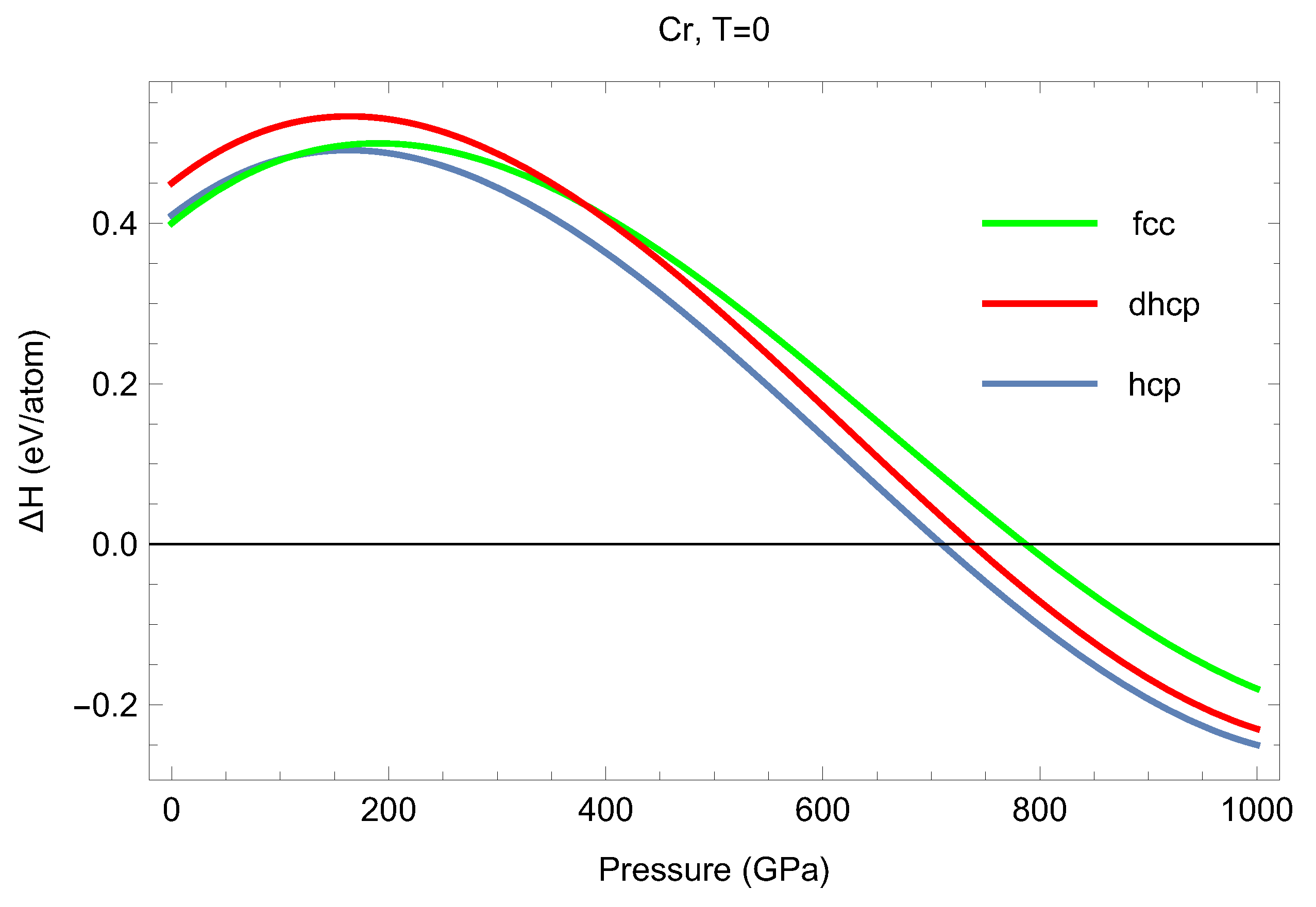
3.1. Cold () Enthalpies of Different Solid Structures of Cr
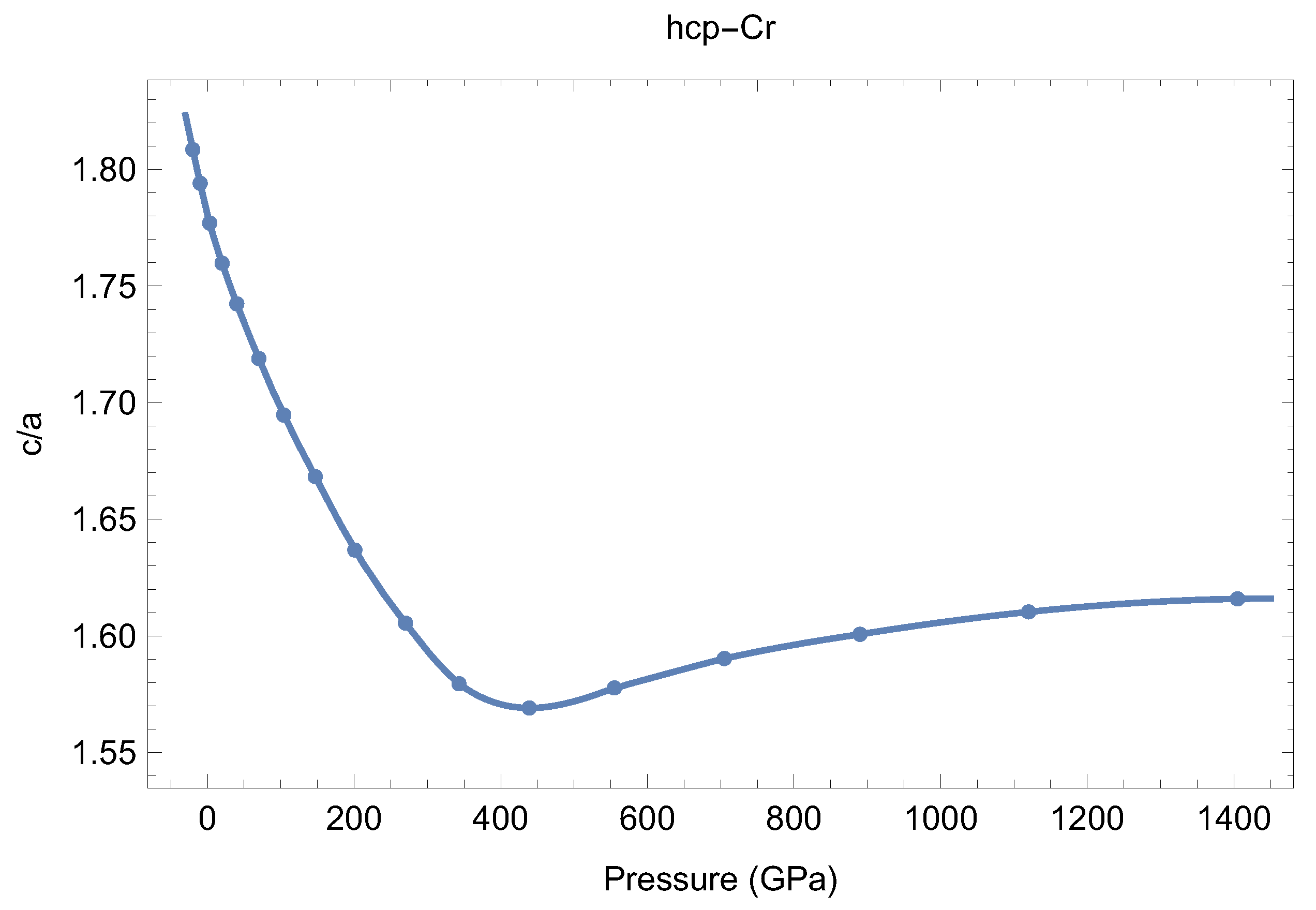
3.2. Equations of State of bcc-Cr and hcp-Cr
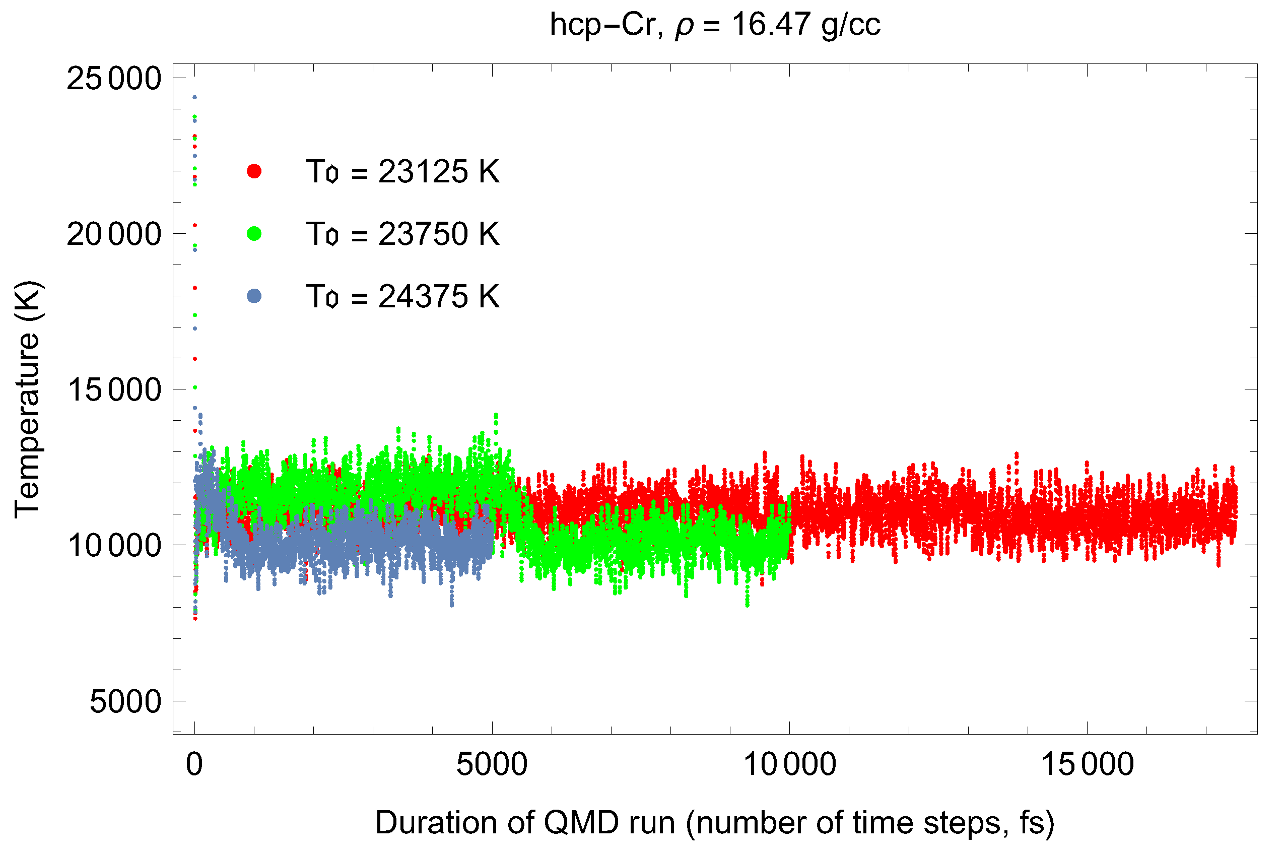
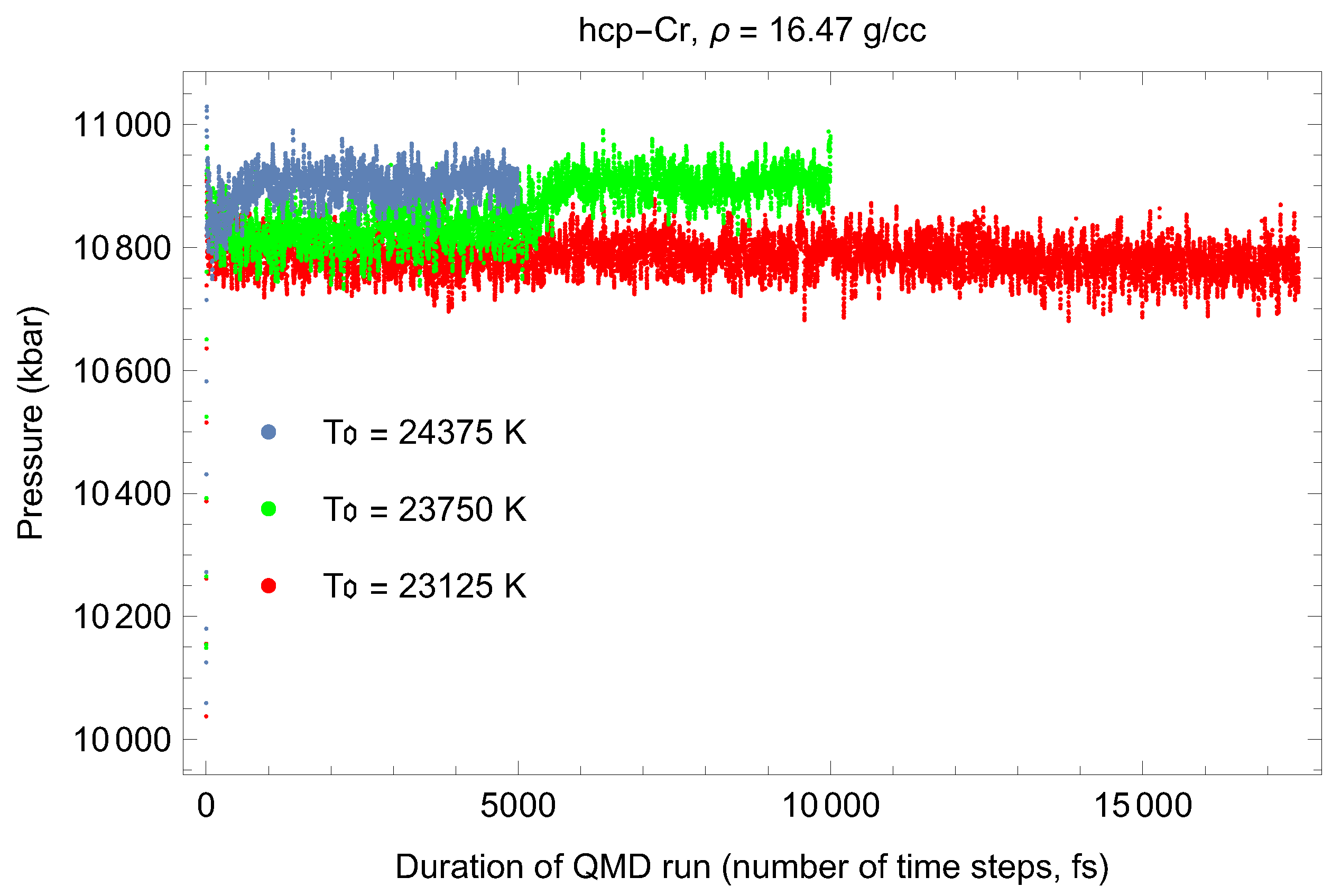
3.3. Ab Initio Melting Curve of bcc-Cr

| Lattice Constant (Å) | Density (g/cm) | (GPa) | (K) | (K) |
|---|---|---|---|---|
| 3.0 | 6.3957 | −5.2 | 1950 | 62.5 |
| 2.8 | 7.8665 | 47.9 | 3330 | 125.0 |
| 2.65 | 9.2793 | 124 | 4460 | 187.5 |
| 2.5 | 11.052 | 266 | 5840 | 187.5 |
| 2.35 | 13.306 | 526 | 7720 | 250.0 |
| 2.25 | 15.160 | 815 | 9310 | 250.0 |
3.4. Ab Initio Melting Curve of hcp-Cr
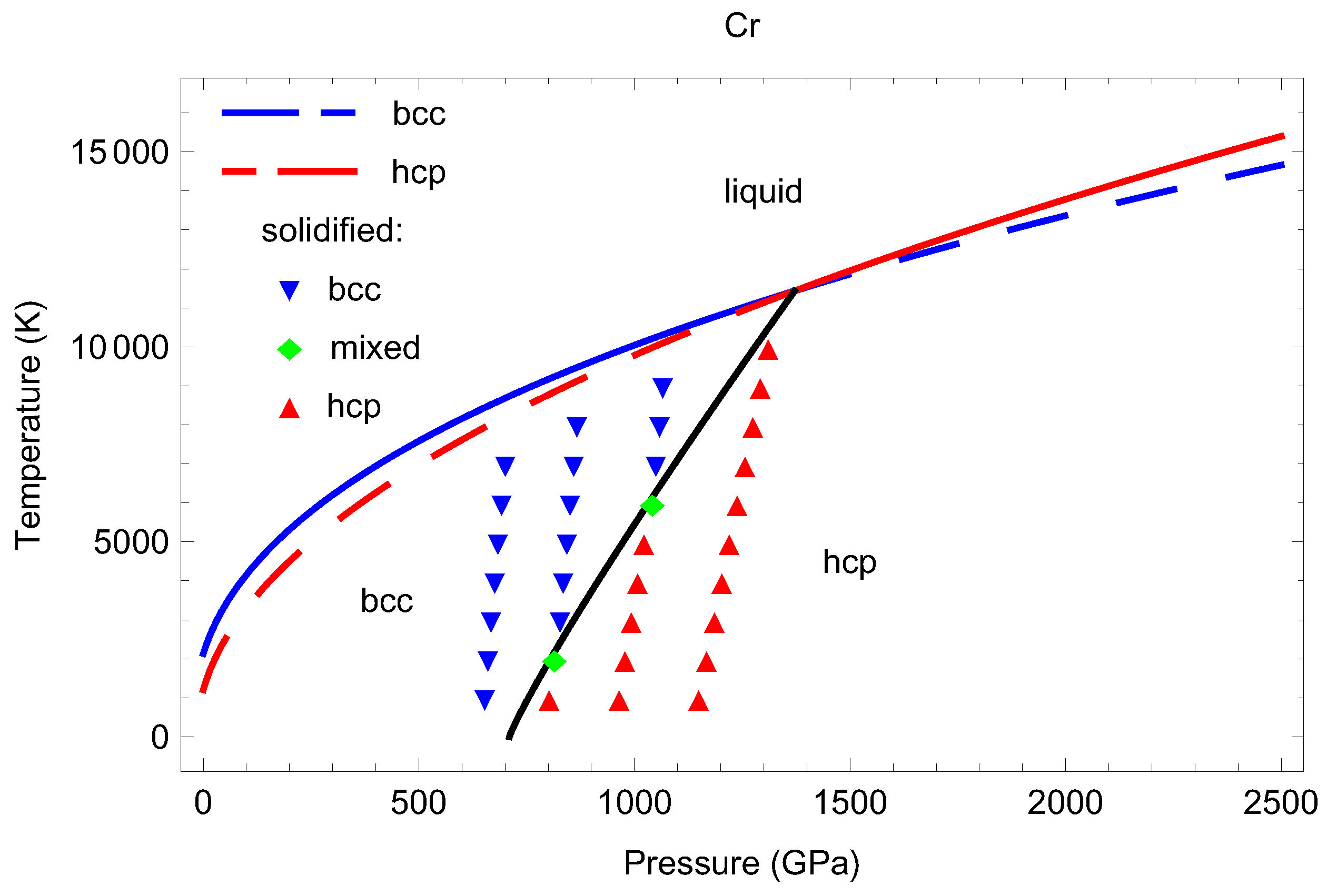
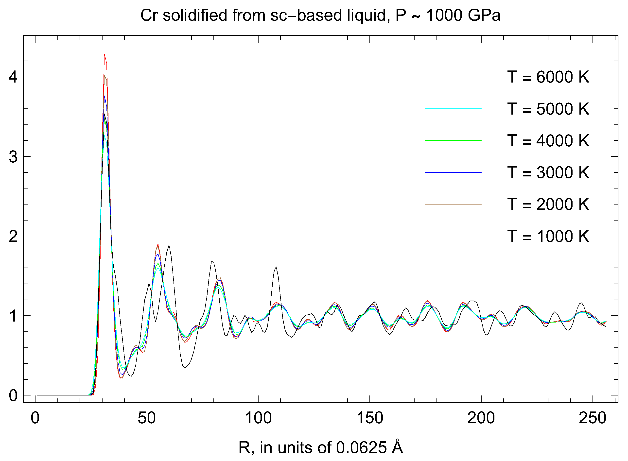
3.5. Inverse-Z Solidification Simulations of Liquid Cr
4. Discussion
5. Conclusions
Author Contributions
Funding
Data Availability Statement
Acknowledgments
Conflicts of Interest
References
- Moynier, F.; Yin, Q.-Z.; Schauble, E. Meteoritic Clues Point Chromium Toward Earth’s Core. Science 2011, 331, 1417. [Google Scholar] [CrossRef] [PubMed]
- Steinitz, M.O.; Schwartz, L.H.; Marcus, J.A.; Fawcett, E.; Reed, W.A. Lattice Anisotropy in Antiferromagnetic Chromium. Phys. Rev. Lett. 1969, 17, 979. [Google Scholar] [CrossRef]
- Asano, S.; Yamashita, J. Ferromagnetism and Antiferromagnetism in 3d Transition Metals. Progr. Theor. Phys. 1973, 49, 373. [Google Scholar] [CrossRef] [Green Version]
- Baty, S.R.; Burakovsky, L.; Preston, D.L. Topological Equivalence of the Phase Diagrams of Molybdenum and Tungsten. Crystals 2020, 10, 20. [Google Scholar] [CrossRef] [Green Version]
- Söderlind, P.; Ahuja, R.; Eriksson, O.; Johansson, B.; Wills, J.M. Theoretical predictions of structural phase transitions in Cr, Mo, and W. Phys. Rev. B 1994, 49, 9365. [Google Scholar] [CrossRef]
- Errandonea, D.; Schwager, B.; Ditz, R.; Gessmann, C.; Boehler, R.; Ross, M. Systematics of transition-metal melting. Phys. Rev. B 2001, 63, 132104. [Google Scholar] [CrossRef]
- Errandonea, D.; MacLeod, S.G.; Burakovsky, L.; Santamaria-Perez, D.; Proctor, J.E.; Cynn, H.; Mezouar, M. Melting curve and phase diagram of vanadium under high-pressure and high-temperature conditions. Phys. Rev. B 2019, 100, 094111. [Google Scholar] [CrossRef] [Green Version]
- Young, D.A. Phase Diagrams of the Elements; University of California Press: Berkeley, CA, USA; Los Angeles, CA, USA, 1991; p. 174. [Google Scholar]
- Lin, R.; Frohberg, M.G. Enthalpy measurements of solid and liquid chromium by levitation calorimetry. High Temp. -High Pres. 1988, 20, 539. [Google Scholar]
- Stankus, S.V. Density of vanadium and chromium at high temperatures. High Temp. 1993, 31, 684. [Google Scholar]
- Dubrovinskaya, N.A.; Dubrovinsky, L.S.; Saxena, S.K. Thermal Expansion of Chromium (Cr) to Melting Temperature. Calphad 1997, 21, 497. [Google Scholar] [CrossRef]
- Gurvich, L.V.; Veits, I.V.; Medvedev, V.A. Calculations of Thermodynamic Properties; Nauka: Moscow, Russia, 1982; pp. 9–12. [Google Scholar]
- Thurnay, K. Thermal Properties of Transition Metals, Forschungszentrum Karlsruhe Report FZKA 6095; INIS: Karlsruhe, Germany, 1998. [Google Scholar]
- Anzellini, S.; Errandonea, D.; Burakovsky, L.; Proctor, J.E.; Turnbull, R.; Beavers, C.M. Characterization of the high-pressure and high-temperature phase diagram and equation of state of chromium. Sci. Rep. 2022, 12, 6727. [Google Scholar] [CrossRef] [PubMed]
- Blöchl, P. Projector augmented-wave method. Phys. Rev. B 1994, 50, 17953. [Google Scholar] [CrossRef] [PubMed] [Green Version]
- Perdew, J.P.; Burke, K.; Ernzerhof, M. Generalized Gradient Approximation Made Simple. Phys. Rev. Lett. 1996, 77, 3865. [Google Scholar] [CrossRef] [PubMed] [Green Version]
- Kresse, G.; Hafner, J. Ab initio molecular dynamics for liquid metals. Phys. Rev. B 1993, 47, 558(R). [Google Scholar] [CrossRef]
- Chen, J.; Singh, D.; Krakauer, H. Local-density description of antiferromagnetic Cr. Phys. Rev. B 1988, 38, 12834. [Google Scholar] [CrossRef]
- Fawcett, E. Spin-density-wave antiferromagnetism in chromium. Rev. Mod. Phys. 1988, 60, 209. [Google Scholar] [CrossRef]
- Wang, C.S.; Klein, B.M.; Krakauer, H. Theory of Magnetic and Structural Ordering in Iron. Phys. Rev. Lett. 1985, 54, 1852. [Google Scholar] [CrossRef]
- Guo, G.Y.; Ebert, H.; Temmerman, W.M.; Schwarz, K.; Blaha, P. Relativistic effects on the structural and magnetic properties of iron. Solid State Comm. 1991, 79, 121. [Google Scholar] [CrossRef]
- Bagno, P.; Jepsen, O.; Gunnarsson, O. Ground-state properties of third-row elements with nonlocal density functionals. Phys. Rev. B 1989, 40, 1997(R). [Google Scholar] [CrossRef]
- Barbiellini, B.; Moroni, E.G.; Jarlborg, T. Effects of gradient corrections on electronic structure in metals. J. Phys. Cond. Mat. 1990, 2, 7597. [Google Scholar] [CrossRef]
- Moroni, E.G.; Kresse, G.; Hafner, J.; Furthmüller, J. Ultrasoft pseudopotentials applied to magnetic Fe, Co, and Ni: From atoms to solids. Phys. Rev. B 1997, 56, 15629. [Google Scholar] [CrossRef]
- Hobbs, D.; Kresse, G.; Hafner, J. Fully unconstrained noncollinear magnetism within the projector augmented-wave method. Phys. Rev. B 2000, 62, 11556. [Google Scholar] [CrossRef] [Green Version]
- Belonoshko, A.B.; Skorodumova, N.V.; Rosengren, A.; Johansson, B. Melting and critical superheating. Phys. Rev. B 2006, 73, 012201. [Google Scholar] [CrossRef]
- Burakovsky, L.; Chen, S.P.; Preston, D.L.; Sheppard, D.G. Z methodology for phase diagram studies: Platinum and tantalum as examples. J. Phys. Conf. Ser. 2014, 500, 162001. [Google Scholar] [CrossRef] [Green Version]
- Burakovsky, L.; Burakovsky, N.; Preston, D. Ab initio melting curve of osmium. Phys. Rev. B 2015, 92, 174105. [Google Scholar] [CrossRef] [Green Version]
- Dubrovinskaia, N.; Dubrovinsky, L.; Solopova, N.A.; Abakumov, A.; Turner, S.; Hanfl, M.; Bykova, E.; Bykov, M.; Prescher, C.; Prakapenka, V.B.; et al. Terapascal static pressure generation with ultrahigh yield strength nanodiamond. Sci. Adv. 2016, 2, 1600341. [Google Scholar] [CrossRef] [Green Version]
- White, G.K.; Smith, T.F.; Carr, R.H. Thermal expansion of Cr, Mo and W at low temperatures. Cryogenics 1978, 18, 301. [Google Scholar] [CrossRef]
- Guo, G.Y.; Wang, H.H. Calculated elastic constants and electronic and magnetic properties of bcc, fcc, and hcp Cr crystals and thin films. Phys. Rev. B 2000, 62, 5136. [Google Scholar] [CrossRef] [Green Version]
- Skriver, H.L. The electronic structure of antiferromagnetic chromium. J. Phys. F 1981, 11, 97. [Google Scholar] [CrossRef]
- Jaramillo, R.; Feng, Y.; Lang, J.C.; Islam, Z.; Srajer, G.; Littlewood, P.B.; McWhan, D.B.; Rosenbaum, T.F. Breakdown of the Bardeen-Cooper-Schrieffer ground state at a quantum phase transition. Nature 2009, 459, 405. [Google Scholar] [CrossRef]
- McQueen, R.G.; Marsh, S.P.; Taylor, J.W.; Fritz, J.N.; Carter, W.J. High-Velocity Impact Phenomena, Chap. VII—The Equation of State of Solids from Shock Wave Studies; Academic Press: New York, NY, USA; London, UK, 1970. [Google Scholar]
- Abrikosov, I.; Ponomareva, A.; Steneteg, P.; Barannikova, S.; Alling, B. Recent progress in simulations of the paramagnetic state of magnetic materials. Curr. Opin. Sol. State Mat. Sci. 2016, 20, 85. [Google Scholar] [CrossRef] [Green Version]
- Dudarev, S.L.; Botton, G.A.; Savrasov, S.Y.; Humphreys, C.J.; Sutton, A.P. Electron-energy-loss spectra and the structural stability of nickel oxide: An LSDA+U study. Phys. Rev. B 1998, 57, 1505. [Google Scholar] [CrossRef]
- Aryasetiawan, F.; Karlson, K.; Jepsen, O.; Schönberger, U. Calculations of Hubbard U from first-principles. Phys. Rev. B 2006, 74, 125106. [Google Scholar] [CrossRef] [Green Version]
- Makeev, V.V.; Popel, P.S. Density and coefficients of thermal expansion of nickel, chromium, and scandium in the solid and liquid states. High Temp. 1990, 28, 525. [Google Scholar]
- Górecki, T. Vacancies and a generalised melting curve of metals. High Temp.-High Pres. 1979, 11, 683. [Google Scholar]
- Nguyen, J.H.; Holmes, N.C. Melting of iron at the physical conditions of the Earth’s core. Nature 2004, 427, 339. [Google Scholar] [CrossRef]
- Available online: https://www.geo.arizona.edu/xtal/geos306/geotherm.htm (accessed on 1 June 2022).
- Dziewonski, A.M.; Anderson, D.L. Preliminary reference Earth model. Phys. Earth Planet. Inter. 1981, 25, 297. [Google Scholar] [CrossRef]
- Xie, Y.-Q.; Deng, Y.-P.; Liu, X.-B. Electronic structure and physical properties of pure Cr, Mo and W. Trans. Nonferrous Met. Soc. China 2003, 13, 5. [Google Scholar]
- He, Y.; Xie, Y.-Q. Electronic structure and properties of V, Nb and Ta metals. J. Cent. South Univ. Technol. 2000, 7, 7. [Google Scholar] [CrossRef]
- Errandonea, D.; Burakovsky, L.; Preston, D.L.; MacLeod, S.G.; Santamaría-Perez, D.; Chen, S.; Cynn, H.; Simak, S.I.; McMahon, M.I.; Proctor, J.E. Experimental and theoretical confirmation of an orthorhombic phase transition in niobium at high pressure and temperature. Comms. Mater. 2020, 1, 60. [Google Scholar] [CrossRef]
- Kaufman, L.; Bernstein, H. Computer Calculation of Phase Diagrams with Special Reference to Refractory Metals; Academic Press: New York, NY, USA; London, UK, 1970; Volume 25, p. 297. [Google Scholar]


| a (Å) | c (Å) | Density (g/cm) | (GPa) | (K) | (K) |
|---|---|---|---|---|---|
| 2.6053 | 4.7355 | 6.2036 | 1.7 | 1270 | 62.5 |
| 2.3593 | 4.0556 | 8.8329 | 129 | 3710 | 125.0 |
| 2.2125 | 3.5521 | 11.468 | 347 | 5860 | 187.5 |
| 2.0737 | 3.2715 | 14.174 | 692 | 8170 | 250.0 |
| 1.9630 | 3.1422 | 16.468 | 1093 | 10190 | 312.5 |
| 1.8565 | 2.9999 | 19.285 | 1744 | 12890 | 312.5 |
Publisher’s Note: MDPI stays neutral with regard to jurisdictional claims in published maps and institutional affiliations. |
© 2022 by the authors. Licensee MDPI, Basel, Switzerland. This article is an open access article distributed under the terms and conditions of the Creative Commons Attribution (CC BY) license (https://creativecommons.org/licenses/by/4.0/).
Share and Cite
Baty, S.R.; Burakovsky, L.; Luscher, D.J.; Sjue, S.K.; Errandonea, D. Ab Initio Phase Diagram of Chromium to 2.5 TPa. Appl. Sci. 2022, 12, 7844. https://doi.org/10.3390/app12157844
Baty SR, Burakovsky L, Luscher DJ, Sjue SK, Errandonea D. Ab Initio Phase Diagram of Chromium to 2.5 TPa. Applied Sciences. 2022; 12(15):7844. https://doi.org/10.3390/app12157844
Chicago/Turabian StyleBaty, Samuel R., Leonid Burakovsky, Darby J. Luscher, Sky K. Sjue, and Daniel Errandonea. 2022. "Ab Initio Phase Diagram of Chromium to 2.5 TPa" Applied Sciences 12, no. 15: 7844. https://doi.org/10.3390/app12157844
APA StyleBaty, S. R., Burakovsky, L., Luscher, D. J., Sjue, S. K., & Errandonea, D. (2022). Ab Initio Phase Diagram of Chromium to 2.5 TPa. Applied Sciences, 12(15), 7844. https://doi.org/10.3390/app12157844