Review

Deep Active Learning for Computer Vision Tasks: Methodologies, Applications, and Challenges

College of Computer, National University of Defense Technology, Changsha 410073, China
*
Author to whom correspondence should be addressed.
Appl. Sci. 2022, 12(16), 8103; https://doi.org/10.3390/app12168103
Submission received: 11 July 2022 / Revised: 8 August 2022 / Accepted: 9 August 2022 / Published: 12 August 2022

Abstract

:
Active learning is a label-efficient machine learning method that actively selects the most valuable unlabeled samples to annotate. Active learning focuses on achieving the best possible performance while using as few, high-quality sample annotations as possible. Recently, active learning achieved promotion combined with deep learning-based methods, which are named deep active learning methods in this paper. Deep active learning plays a crucial role in computer vision tasks, especially in label-insensitive scenarios, such as hard-to-label tasks (medical images analysis) and time-consuming tasks (autonomous driving). However, deep active learning still has some challenges, such as unstable performance and dirty data, which are future research trends. Compared with other reviews on deep active learning, our work introduced the deep active learning from computer vision-related methodologies and corresponding applications. The expected audience of this vision-friendly survey are researchers who are working in computer vision but willing to utilize deep active learning methods to solve vision problems. Specifically, this review systematically focuses on the details of methods, applications, and challenges in vision tasks, and we also introduce the classic theories, strategies, and scenarios of active learning in brief.

1. Introduction

With the rapid development of deep learning, the performance of computer vision tasks has achieved breakthroughs benefiting from large-scale annotated datasets, such as ImageNet [1], Cityscapes [2], and AbdomenCT-1K [3]. These datasets provide direct supervision for model training. Meanwhile, there are useless, uninformative examples, which serve as risks to overwhelm the training. Apart from the noise inside the labeled data, there are always scenarios where unlabeled data is abundant. However, manual labeling is high cost, such as medical image analysis, autonomous driving, anomaly detection, and related issues in computer vision tasks. Specifically, taking the Cityscapes [2] dataset as an example, the pixel-wise annotation will cost more than 90 min per image in the urban street segmentation task. Similarly, in the medical image tumor segmentation task, it is more challenging for medical experts to detect the mm-size objects from 3D volume data, which is more time-consuming and medical knowledge–demanding.
Under the above conditions, maximizing the model’s performance with a limited annotation budget becomes the primary concern. In order to figure out this problem, active learning becomes a promising solution to improve data efficiency and relieve the high annotation burden. As a subfield of machine learning, the core idea of active learning [4] is to find the most valuable samples through some heuristic strategies, so the model can achieve or even exceed the expected performance with as few labeled samples as possible. The intuition of active learning is that not all samples in a dataset have the same significance for model training. For example, some samples contain more noise that hinders training. Besides this, some samples are too similar to be worth labeling. Therefore, the goal of active learning is to select as few valuable or ambiguous samples as possible via the designed strategy and promote the performance with the selected samples interactively. The above iterative training process between optimization and annotator is the primary active learning mechanism, and human annotations exist in each training interaction. Consequently, the essence of active learning is the Human-in-the-Loop (HITL) computing systems, where human expertise is joint in the computer-based systems [5]. Humans (such as doctors in clinical diagnosis) are part of the intelligent system and participate in the model training process by providing judgments or domain-knowledge that influence the final output of the system [6]. More details are introduced in Algorithm 1 and other surveys [5,6].
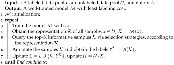
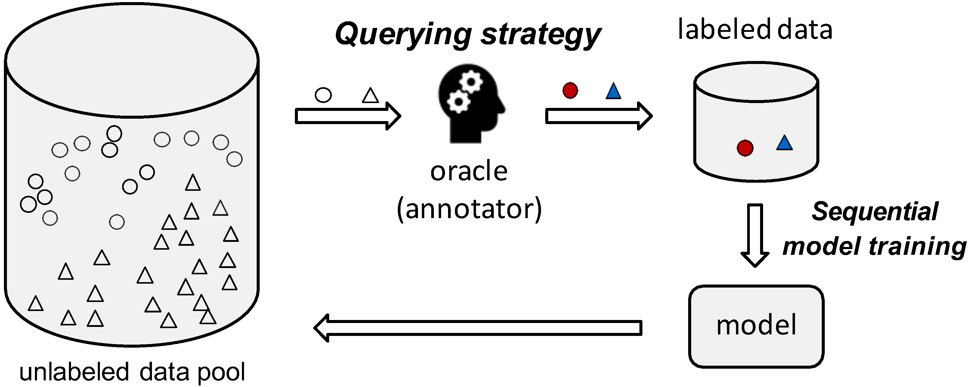
Algorithm 1: The pool-based active learning workflow
Applsci 12 08103 i001
Settles’s active learning literature survey [4] systematically summarized classic active learning methods in 2004. More basic definitions and formulations can be found in this survey [4]. Active learning has been rapidly growing and booming with various novel methodologies, applications and challenges in recent years. Settles’s survey provided the basic theory for active learning, especially the traditional AL. Differently, our work focuses on deep learning–based active learning theories in computer vision tasks, which is named deep active learning in this paper.
Apart from this, we summarize the latest surveys [6,7,8,9] about deep learning in Table 1. Previous surveys systematically introduced the deep active learning in many fields, such as CV and NLP. After studied the existing surveys about deep active learning and their references, we found that there was not any review designed for CV researcher. Hence, we decided to re-organize existing works and introduce latest research from a CV-related perspective in this manuscript. The biggest difference between this manuscript and above-mentioned works is that the expected audience of this review are researchers who are working in computer vision but willing to utilize deep active learning methods to solve CV problems. Active learning is still new to them. As such, we organized this manuscript from the perspective of a CV researcher, and introduced the deep active learning from CV-related methodologies and corresponding applications. This CV-friendly survey is our new contribution to the community.
The remainder of this review is as follows: First, we argue that it is necessary to introduce the basic concepts and methodologies of traditional active learning for the newcomers. Then, Section 2 introduces the three basic candidate selection strategies in active learning and give responding examples, and then we detail the pool-based strategy. Section 3 introduces the common querying scenarios in active learning. Then, we focus on the methodologies integrated deep learning and active learning. Section 4 details the recent methodologies for deep learning-based active learning. Section 5 details the applications of deep active learning, especially in computer vision tasks. Finally, Section 6 summarizes the existing challenges of deep active learning in computer vision tasks, which are the future works in this field. Section 7 concludes the survey.

2. Candidate Selection Strategies in Active Learning

In the classic active learning framework, one of the two most important components is how to develop a criterion for evaluating the “worthiness” of unlabeled samples. After evaluation, the selection strategies decide whether one sample is worthy of being labeled by the annotator according to its worthiness. The selected samples are regarded as candidates. Finally, an appropriate selection strategy reduces the labeling cost and thus has important implications in active learning. Due to this knowledge being beyond the main concern of this review, Table 2 introduces four basic selection strategies in brief, and more details can be found in existing active learning surveys [6,7,8,9].

2.1. Random Selection Strategies

Random sampling uses random numbers to select samples from the unlabeled dataset for labeling. There is no interaction with the model’s prediction in the above process, which is the most naive selection strategy. Consequently, it is often used as the basic comparison experiment in active learning.

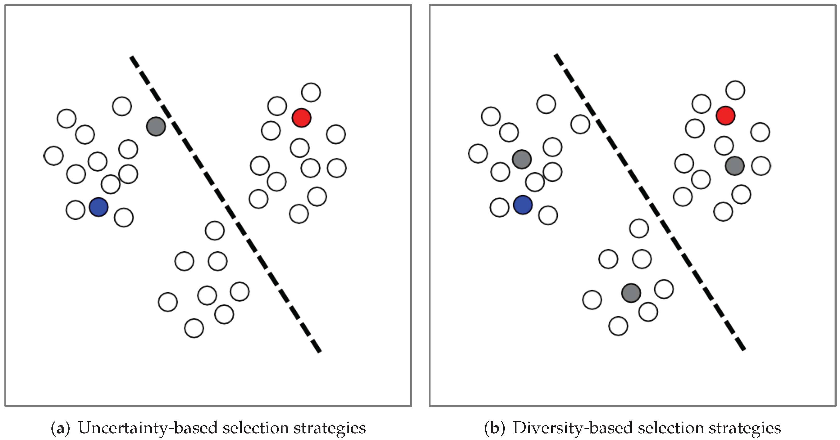
2.2. Uncertainty-Based Selection Strategies

The uncertainty-based selecting method is the simplest and most common strategy, which assumes that the samples closest to the classification hyperplane have richer information than others. It selects the most uncertain samples according to the predicted value of the samples by the current model.
Typical uncertainty-based selection strategies includes Least confidence, Margin sampling, Multi-class level uncertainty, and Maximize entropy. This survey briefly summarized the above strategies in Table 2. More details can be found in existing surveys [6,7,8,9]. Consequently, the machine learning model can quickly improve its performance by learning the labels of the samples with substantial uncertainty.

2.3. Diversity-Based Selection Strategy

The above uncertainty-based selection strategy can effectively sample a single candidate for annotation, but it is often ineffective when there are multiple candidates. At this time, the selection strategy based on the diversity of sample feature distribution comes into being. Diversity tends to reflect the prediction consistency among the samples, i.e., higher diversity values denote more inconsistency between the candidate sample and the entire unlabeled pool [26]. Typical diversity-based measurement strategies includes angles-based and redundancy-based perspectives. We also summarized above strategies in Table 2 and provided the comparison between uncertainty-based and diversity-based selections in Figure 1.

2.4. Committee-Based Selection Strategy

Committee-based selection strategy [23] is based on version space reduction, and its core idea is to preferentially select unlabeled samples that can reduce the version space to the greatest extent. The committee-based selection strategy’s motivation is that the most informative selections are the samples where the committee predicts the most inconsistent. Typical committee-based selection strategies include vote entropy and average KL divergence, which are listed in Table 2. There are four basic steps in the committee-based selection strategy:
  • Multiple models M 1 , , M N are used to construct a committee C for voting, i.e., C = M 1 , , M N .
  • The models in the committee C are then trained on the labeled dataset L and get different parameters.
  • All models in the committee make predictions separately on unlabeled samples from U . The samples with the richest information are voted.
  • The samples which obtain the most disagreements are selected as candidates for labeling.

3. Common Querying Scenarios in Active Learning

According to the application scenarios, active learning methods can be divided into three types: query synthesis scenario, stream-based scenario, and pool-based scenario. We briefly summarize the above querying scenarios in Table 3 and introduce the pool-based scenario in detail.
Among the above mainstreams, pool-based active learning is more compatible with batch-based modern deep learning training mechanisms. Compared with the stream-based selective sampling, the pool-based scenario is able to consider every sample based on this batch comprehensively. Consequently, it has become the most common scenario in computer vision tasks. Moreover, the most related works introduced in this review also belong to the pool-based active learning scenario.
Figure 2 is a classic pool-based active learning framework. A single batch of unlabeled samples is input to the model from the unlabeled data pool during the training process. Then, the query strategy selects the most valuable samples for labeling according to the informativeness. After that, these labeled samples are added to the labeled dataset to continue training the model.
Sequentially, we formally define the pool-based active learning method in Algorithm 1. The End conditions include that the performance of the model meets requirements, or the budgets for annotation run out, or the selected samples are hard for annotators to label.
As shown in Figure 2, there are the labeled pool L = { ( x 1 l , y 1 l ) , , ( x N l l , y N l l ) } and the unlabeled pool U = { x 1 u , , x N u u } at the beginning. N l and N u are the number of labeled and unlabeled samples, respectively. Then, the data from the labeled pool is fed into the machine learning model for supervised training. After that, the well-trained model is utilized to extract the representation R u = { ( r 1 u ) , , ( r N u u ) } of the unlabeled pool data. Based on R u , the informativeness is calculated according to the query strategy. The top-K samples K = { x 1 k , , x N k k } are selected out to the oracle (human annotators) and obtain the labels Y K = { y 1 k , , y N k k } . Finally, the labeled pool L will be updated to L = { ( x 1 l , y 1 l ) , , ( x N l l , y N l l ) , ( x 1 k , y 1 k ) , , ( x N k k , y N k k ) } . With the updated L, the machine learning model will promote the performance in return. Meanwhile, the size of unlabeled pool U is reduced to N u N k . The above loop will be repeated until one of the end conditions is met. Since the selected samples K from the unlabeled pool U are the most significant ones for training, the size of L to learn a model can often be much smaller than the size required in classic supervised learning without active learning.

4. Deep Active Learning Methods

Recent developments are dedicated to multi-label active learning, hybrid active learning, and deep learning–based active learning. In the upcoming sections, we will detail deep learning–based active learning.

4.1. Deep Active Learning for CNNs

As we introduced in Section 2.2, uncertainty is one of the most used metrics to select candidate in active learning. We summarize the uncertainty estimation methods in Table 4. At the same time, Bayesian methods are known for their ability to capture underlying model uncertainty. The classic Bayesian active learning framework consists of an unlabeled data pool U , the labeled data pool L, and a Bayesian model M trained on the current L. The output of the Bayesian model M is p ( y | x , M , L ) , where the input data is x and the prediction y { 1 , . . . , c } in the classification tasks. In Bayesian deep learning, the model M is replaced by a Convolutional Neural Network (CNN) with prior probability distributions. Gal et al. [38] proposed a Bernoulli-based approximate variational inference method. After that, they [39] proposed to capture model uncertainty by using the Monte Carlo dropout regularization as a variational Bayesian approximation. Consequently, it is natural to utilize Bayesian methods to actively select valuable candidates.
Gal et al. [40] introduced the Bayesian Convolutional Neural Networks into the active learning framework. They demonstrated that such combination improved performance over existing active learning methods on the image classification dataset MNIST [41] (achieving 5% test error) and skin cancer diagnosis dataset ISIC 2016 [42] (achieving 0.71/0.75 AUC). Bayesian Active Learning by Disagreement (BALD) [43] was proposed to be the basic selection strategy, where Shannon entropy [44] was utilized to measure the “information content”. The discrepancy of Shannon entropy denoted the difference between the information entropy of a certain sample and the average information entropy of the dataset. The larger the difference, the more information the sample contained relative to the average. Finally, the BALD strategy pushed the samples with the largest Shannon entropy. The above process is formulated as follows.
X = arg max x U I ( x ) = arg max x U S E ( y x , L ) E θ P ( θ L ) [ S E ( y x , M ) ] ,
where I ( · ) is the mutual information. Higher mutual information means the model’s predictions are more uncertain. S E ( y x , L ) and S E ( y x , M ) are represented by the Shannon Entropy of the prediction P M ( y x ) and the mean distribution P M ( y L ) , respectively.
Ensemble learning is a well-known technique in machine learning that improves performance by integrating different models and combining their results [45]. Ref. [46] explored the difference between ensemble-based methods against Monte Carlo dropout methods on image classification tasks MNIST [41] (achieving 90% test set accuracy with roughly 12,200 labeled images), CIFAR-10 [47] (achieving 91.5% accuracy) and diabetic retinopathy (DR) detection (https://www.kaggle.com/competitions/diabetic-retinopathy-detection/rules, accessed on 9 July 2022) (achieving 0.983 AUC). They conducted extensive experiments from 11 aspects and found that the former outperformed the latter and was a more reliable measure of uncertainty.
Bayesian-based methods addressed the problem of uncertainty-based candidate selection strategies, but there was another obstacle that needed to be solved. The biggest difference of CNN-based deep learning (DL) methods and traditional active learning (AL) methods is that AL methods query candidates one by one while DL methods load a batch size of samples at the same time. Ozan Sener and Silvio Savarese [48] conducted experiments on vision tasks with traditional active learning methods and found that previous AL works did not perform well for CNN-based vision tasks due to the batch settings during model training. They attributed this ineffectiveness to batch sampling. In order to solve it, they defined the active learning as a Core-Set selection problem, where the algorithm aims to train on a small mount of labeled samples instead of the whole dataset such that the trained model is able to get competitive performance over the model trained on the whole dataset. They defined the core-set selection problem as the following optimization:
min L 1 : L 1 b 1 n i [ n ] l o s s x i , y i ; M L 0 L 1 1 L 0 + L 1 j L 0 L 1 l o s s x j , y j ; M L 0 L 1 ,
where L 0 represents the randomly selected samples at the beginning, L 1 represents newly selected samples from the entire dataset under budget b. n is the number of samples in the entire dataset. M L 0 L 1 denotes the trained model under the subset L 0 and L 1 . l o s s is the loss function, where the authors suggested the cross-entropy loss for effective training. In order to prove their hypothesis, they conducted experiments on active learning for fully supervised models and weakly supervised models. Specifically, they used dataset CIFAR10/100 [47] for image classification and dataset SVHN [49] for digit classification.
Based on the Core-Set strategy, the combination of batch-based active learning and deep learning has been a researcher topic in the community. the goal of batch-based deep active learning is to select the most informative batch or mini-batch B * = x 1 * , x 2 * , , x n * from the loaded batches B , where B belongs to unlabeled pool U , and n is the batch size. We formulate above process as follows.
B * = arg max B U Φ B , M ( L ) ,
where Φ ( · ) is the score function to measure the informativeness of the batch B , L is the labeled data pool, M is the trained model.
After that, most of the related research was devoted to the innovation of the scoring function Φ ( · ) . David Janz et al. [50] adopted the idea of Bayesian Active Learning by Disagreement (BALD) [43] into scoring function. Specifically, they utilized the mutual information I ( · ) as score function and selected samples with the maximum gain of information, where Φ B A L D ( B , M ( L ) ) = i = 1 n I y i ; M x i , L . However, BALD just considered the mutual information between one single sample x i and model parameters M ( L ) , and did not take the relationship between samples in an batch. As an extension of BALD, BatchBALD [51] promoted the BALD by estimating the mutual information I ( · ) between all samples in an batch and the model, which was formulated as Φ B a t c h B A L D ( B , M ( L ) ) = I y 1 : n ; M x 1 : n , L .
Yoo et al. [52] proposed a novel loss prediction module into the target model. This module consisted of global average pooling (GAP), full connected layer (FC) and ReLU, capturing multi-level features. Then the features was concentrated and calculated the loss prediction. All unlabeled samples were evaluated by this module via mini-batch. The batch with the top-K predicted losses selected as candidates and then labeled to update training set. the proposed module was evaluated in Image Classification task CIFAR-10 [47] (achieving accuracy of 0.9101), Object Detection task PASCAL VOC [53] (achieving 0.7338 mAP), and Human Pose Estimation task MPII [54] (achieving 0.8046 [email protected]).

4.2. Generative Adversarial Active Learning

According to the analysis of [55], the Core-Set strategy [48] is very inefficient in high-dimensional representation learning due to its inherent distance-based computation. This obstacle is well addressed by leveraging GAN or VAE for representation learning from high-dimensional data.
Generative Adversarial Networks (GAN) is a novel representation learning method proposed by Goodfellow [56]. Its core idea is “Generative” and “Adversarial”. The GAN network structure contains two models. One is the generator G and the other is the discriminator D . The generator generally uses a deconvolutional neural network or a fully connected neural network to synthesize new data (e.g., images). At the same time, the discriminator is a CNN-based binary classifier to distinguish whether the input is from the natural distribution or synthesized one from the generator.
The discriminator is trained first to make a good judgment so that the real and generated samples can be better distinguished. Then the parameters of the generator can be updated more accurately. The goal of discriminator is that P ( D ( x ) | x r e a l ) = 1 while P ( D ( x ) | x f a k e ) = 0 . Then the generator and discriminator in GANs are trained against each other in a two-player game. The weights and biases of the discriminator and generator are trained through back-propagation until they reach a dynamic equilibrium state with unlabeled samples. In order to discriminate samples and classify them, the discriminator usually utilizes the cross-entropy loss to measure similarity, which is formulated as follows [56]:
L D = 1 N i = 1 N log D x ( i ) + log 1 D G z ( i )
L G = 1 N i = 1 N log 1 D G z ( i )
z p z ( z ) is the generated distribution and x p data ( x ) is the real distribution. N denotes the batch size. As a consequence, the objective function of GAN is shown as follows [56]:
L = arg min G max D V ( G , D ) = E x p data ( x ) [ log D ( x ) ] + E z p z ( z ) [ log ( 1 D ( G ( z ) ) ) ] ,
where V ( G , D ) is the difference between the generated distribution p z and the actual distribution p data . max is to train the discriminator to discriminate the sample to the greatest extent. min is to train the generator to minimize the difference between the generated sample and the actual sample. When the algorithm converges, the samples generated by the generator can confuse the discriminator and cannot distinguish right from wrong. In other words, the generator should try its best to generate more realistic results to deceive the discriminator. The discriminator should try its best to distinguish the truth from the false and not be deceived by the generator. The network reaches the ideal state when the generated result is actual (discrimination probability is 0.5).
Zhu et al. [57] firstly proposed a novel query synthesis-based active learning method GAAL fused with GAN. GAAL was trained on datasets MNIST [41] (achieving accuracy 70.44%) and CIFAR-10 [47] while tested on the dataset USPS [58]. The workflow of GAAL can be concluded as Algorithm 2.
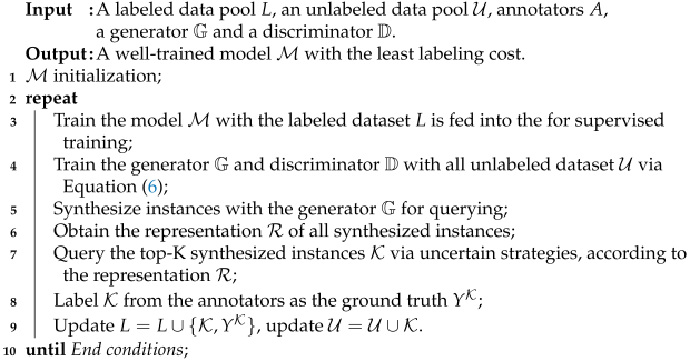
Algorithm 2: The synthesis-based active learning method workflow
Applsci 12 08103 i002
GAAL inspired GAN-based generative adversarial methods in active learning. Consequently, the latter works were devoted to studying pool-based Generative Adversarial Active Learning. Tran et al. [59] proposed a framework of Bayesian Generative Active Learning (BGAL) to solve multi-classification tasks when the amount of labeled data is small. The proposed BGAL was validated on MNIST [41] (achieving accuracy 99.68%), CIFAR-10/100 [47] (achieving accuracy 91.13%), and SVHN [49] (achieving accuracy 69.69%). Mayer et al. [60] proposed a pool-based active learning strategy(ASAL). Compared to traditional pool-based strategies for exhaustive uncertainty search from unlabeled pools, ASAL utilized GAN to generate the most representative samples from unlabeled pools, resulting in more efficient active learning techniques. ASAL was validated on the datasets MNIST [41] (reducing 300 labeled samples), CIFAR-10 [47] (reducing 500 labeled samples), CelebA [61] (reducing 750 labeled samples), SVHN [49], and LSUN Scenes [62]. Sinha et al. [63] proposed a pool-based semi-supervised active learning algorithm VAAL. VAAL obtained great improvement in experimental results on classification and segmentation. VAAL achieved great improvement in experimental results, including CIFAR10/100 [47] (achieving accuracy of 90.16%/63.14%), Caltech-256 [64] (achieving 1.01% improvement on Core-set), ImageNet [1], Cityscapes [2] (achieving mIoU 62.95), and BDD100K [65] (achieving mIoU 44.95).
The above methods were devoted to directly generating the representative samples by solving some optimization problems, and then improving the efficiency of screening samples for active learning. More details are summarized in Table 5. Apart from that, Huijser et al. [66] firstly proposed to use a GAN to generate a batch of samples along the decision boundary of the current classifier. Next, they determined the location where the category changed from the generated samples through visualization and added it to the set of samples to be labeled. Finally, the method’s effectiveness was verified by a large number of image classification experiments. The method can reduce the burden of data annotation by requiring the annotator to label decision boundaries instead of samples.

4.3. Semi-Supervised Active Learning

Vision tasks based on supervised learning require a large amount of labeled data for model training. These labeled data not only provide direct supervision signals but also limit the generalization ability of the model [69]. At the same time, the acquisition of these data is challenging due to the cost and time of annotation [26]. To alleviate this limitation, methods based on semi-supervised learning have become another mainstream. It studies model training under the premise of limited labeled data. It expects higher performance to balance the dilemma between performance and cost, which is a perfect fit for active learning, thus bringing a lot of research and practical value.
Semi-supervised learning (SSL) can train the model with a small amount of labeling cost. Unlike active learning, SSL methods usually select samples with confident prediction results instead of uncertain samples and then label them directly by the model instead of annotators. However, it is still impossible to guarantee that these high-confidence prediction results do not contain noise or erroneous results due to model prediction accuracy errors. Thus, these predictions could not directly participate in model training because the pseudo-labels may make the model abnormal. In contrast, active learning selects the samples with the most uncertain prediction results to be labeled by annotators, which can be used as the ground truth without noise and thus ensure the quality of labels. Therefore, the combination of semi-supervised learning methods and active learning methods can complement each other to a certain extent.
McCallumzy et al. [70] firstly proposed the above idea that combined Query-by-Committee active learning and Expectation-Maximization (EM) algorithms, using the naive Bayes method as a classifier and conducting experiments on text classification tasks. Subsequently, Muslea et al. [71] promoted the above work and proposed the joint testing method (Co-Testing), where two classifiers were trained in different perspectives. After that, samples were jointly selected for annotation. Finally, new labeled data were joined into the expectation-maximization (Co-EM) algorithm. Sequentially, Zhou et al. [72] combined the above semi-supervised learning and active learning methods and then validated that both of them are beneficial to the image retrieval task.
In addition, the self-training algorithm is one of the primary methods in SSL, and its core steps are shown in Algorithm 3. Firstly, the self-training algorithm initializes the model with a small number of labeled samples to ensure the initial performance of the model. Then, the algorithm selects appropriate samples and calculates their corresponding predicted labels based on the predicted representations. Finally, the labeled dataset is updated with new pseudo-labeled samples and the model is trained again in the next iteration. The main challenge of the semi-supervised learning algorithm is that SSL is easy to introduce a large number of noise samples during the training process, so the model cannot learn the correct information. Some researchers mitigate noisy samples by constructing Co-Training [73] and Tri-Training [74] algorithms of multiple classifiers.
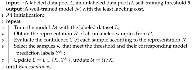
Algorithm 3: The workflow of basic self-training algorithm
Applsci 12 08103 i003
Apart from this, the authors of Refs. [75,76,77] integrated semi-supervised learning and active learning skillfully. They combined uncertainty-based selection strategies and self-training methods and made full use of their respective advantages while making up for their shortcomings. Consequently, their works achieved remarkable results.
However, the above semi-supervised active learning methods have not dealt with the noisy samples effectively, so it still had a significant impact on the model.
Song et al. [78] combined active Learning and semi-supervised Learning with inconsistent prediction and utilized data augmentations. These works achieved remarkable performance in CIFAR-10/100 [47] (improving 1.47%/1.16% accuracy) and SVHN [49] (improving 0.43% accuracy) classification tasks. However, they still suffered from data augmentation because there were too little data augmentations to estimate inconsistency. Sequentially, Guo et al. [79] proposed REVIVAL method and obtained more semantic distribution information via learning the continuous local distribution of unlabeled samples from feature space.
Despite the progress, most active learning algorithms suffer from data waste problems because they ignore that most of the data in unlabeled pool is not actively annotated, which can further enhance the performance via semi-supervised learning (SSL).

4.4. Active Contrastive Learning

Semi-supervised learning still needs some labeled data to carry out training, but self-supervised learning extracts representation by mining data instead of annotation. Contrastive learning is one of the most successful paradigms for self-supervised learning. The key idea of contrastive learning is to learn its relationship by comparing the similarity of different samples in the dataset. Thus, how to define the positive pairs (similar samples) and negative pairs (dissimilar samples) is the main issue in contrastive learning. The workflow of basic contrastive active learning is reported in the Algorithm 4. For arbitrary data x, the goal of contrastive learning is to learn an encoder f ( · ) such that:
score f ( x ) , f x + > > score f ( x ) , f x ,
where f ( x ) denotes the global features. f ( x + ) denotes the local features from positive samples. f ( x ) denotes the local features from negative samples. The score ( X 1 , X 2 ) is the function to measure the similarity of vectors X 1 and X 2 . Euclidean distance and cosine similarity are two classical score functions, which are formulated as follows.
E u c l i d e a n X 1 , X 2 = F X 1 F X 2 2
C o s i n e X 1 , X 2 = X 1 T X 2 | X 1 | | X 2 |
After that, it optimizes an objective that pulls the positive pairs together while pushing the negative pairs away in the representation space. The loss function InfoNCE [80] is usually used in the related research of contrastive learning, which is formulated as follows:
L N C E = E X log s c o r e f ( x i ) , f x i + s c o r e f ( x i ) , f x i + + j i s c o r e f ( x i ) , f x j ,
where the corresponding sample x has one positive and N − 1 negative pairs. By minimizing the InfoNCE loss, contrastive learning is to make the features of f ( x ) more similar to the features of positive samples f ( x + ) , and less similar to the features of N − 1 negative samples f ( x j ) ( j 1 , , N 1 ). Finally, it can maximize a lower bound on the mutual information between f ( x ) and f ( x + ) [81].
McAllester et al. [82] analyzed the theoretical shortcomings of contrastive learning, where they argued that the learned representations of contrastive learning were high relative to the size of negative samples. For example, MoCo [83,84,85] and SimCLR [86,87] obtained success due to the various data argumentation with large memory bank and extremely large batch size, respectively. However, Saunshi et al. [88] validated that a larger size of negative samples does not always learn better representations, leading to better performance. They found that the larger batch size would likely generate more redundant samples, thus affecting the efficiency of contrastive learning.
In order to address the above problems, active learning was introduced into contrastive learning by assisting the selection of negative samples [89]. When they carried out the cross-modal contrastive representation learning, uncertainty and diversity were used to sample the negative samples, thus reducing the redundancy actively.
Furthermore, previous active learning works assume that the labeled and unlabeled data pools follow the same class distribution. When applying these works to mismatched class distribution tasks, it suffered from performance degradation sharply. Du et al. [90] focused on this problem. They firstly defined the score function:
s c o r e = θ x i , x j = exp f x i f x j τ · f x i f x j
Then, they used contrastive learning to select semantic and distinctive features and then selected the most informative unlabeled samples v with minimax selection scheme for querying.
v = argmin v i V L max v j N ( i ) d x i , x j ,
where d ( x i , x j ) calculates the Euclidean distance between embeddings of two nodes x i and x j , N ( i ) represents the neighbor set of node i, V and L denotes the node set and labeled set, respectively. Finally, they generalized contrastive learning to active learning with the following modified loss function:
L C A L x i , x i = log θ x i , x i + λ · x p P ( i ) θ x i , x p θ x i , x i + λ · x p P ( i ) θ x i , x p + j i θ x i , x j + θ x i , x j ,
where P ( i ) denotes the set of positive embedding whose label is the same with node v i .
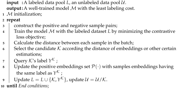
Algorithm 4: The workflow of basic contrastive active learning algorithm
Applsci 12 08103 i004
Zhu et al. [91] integrated graph neural networks (GNNs)-based active learning with contrastive learning. They denoised the selected candidates by considering the neighborhood propagation scheme in GNNs. Krishnan et al. [92] proposed the featuresim score, which selected balanced, diverse, and informative samples (samples in-between clusters and from edge of clusters) from each class. Gao et al. [93] applied active learning and contrastive learning to the fine-grained off-road semantic segmentation task. They used different semantic attributes for weak supervision and defined the image patches that share the same label as positive pairs while the rest were negative pairs. Besides this, they proposed a risk evaluation method to evaluate high-risk predictions and selected for additional annotation.

4.5. Other Deep Active Learning

Unsupervised domain adaptation (UDA) is a type of cross-domain transfer learning, where the source samples are annotated, and the labels of target samples are absent during training [94]. The goal of UDA is to minimize the discrepancy in distribution between the source domain and the target domain and to learn a robust generalized representation without target annotations [95]. At present, only a few works [96,97] have utilized active learning methods to solve domain adaptation challenges and to improve the performance of the source domain model in the target domain. Recently, Ning et al. [98] first proposed a novel framework that combines active learning and unsupervised domain adaptation to assist cross-domain semantic segmentation tasks. Specifically, they clustered multiple anchors from the source domain to adopt the multi-center distribution. After that, they queried from the unlabeled target samples to the most complimentary samples from the source domain as candidates. The active learning method modeled the data distribution in both the source and target domain and, thus, captured more comprehensive information for domain adaptation.

5. Applications

Recently, computer vision is achieving a breakthrough with deep learning and booms wide applications, which require large amounts of labeled data. Meanwhile, it is impossible to abandon labels entirely or give up unlabeled data in practical applications. Under this condition, active learning can provide a more reasonable expedient, i.e., to annotate valuable data instead of all data.
According to the detailed introductions of deep active learning in the previous sections, we can conclude that the deep active learning methods can play a significant role in the label-intensive vision tasks, helping to reduce labeling costs. In other words, active learning applications are for such conditions, i.e., how to save the workload of labeling and make the model achieve satisfactory performance under a large amount of unlabeled data. Here, we only introduce some extensive-studied applications related to active learning, especially deep active learning.

5.1. Deep Learning-Based Autonomous Driving

In supervised deep learning, a large amount of labeled data needs to be collected for training [99,100], especially in the scorching field of autonomous driving. In this field, the perception of the environment of unmanned vehicles is particularly important [101,102]. The perception of the model directly affects the quality of decision making and plays a vital role in the safety of unmanned vehicles [103,104]. However, there are many complexities environments in autonomous driving scenes. In order to ensure the performance of the model, most companies need to collect the images, point clouds, and radar data from the actual scene for training. Such massive amounts of data are challenging to collect and label. Nevertheless, active learning is able to select the most valuable samples (or via the uncertainty estimation of the current model prediction) and then manually label them. Finally, we can carry out continued model training, thereby improving the model’s performance as much as possible, improving stability and security. In this section, we introduce and compare the applications on deep active learning–based autonomous driving. The overview is summarized in the Table 6.
Hussein et al. [105] introduced active learning into the autonomous navigation application. In order to address the challenge of generalizing a model over unseen data, they utilized the entropy to measure the confidence of prediction and then labeled the low-confident samples for iterative training. Dhananjaya et al. [106] focused on the harsh weather and low light conditions during driving. They proposed a related dataset containing 60k images from videos, which consisted of various weather conditions (clear, rain, and snow), light levels (bright, moderate, and low), and street types (asphalt, grass, and cobblestone). Under the proposed dataset, previous deep learning–based autonomous driving algorithms suffered from accuracy degradation. The authors introduced an active learning framework to reduce the redundancy from adjacent frames in the video and find the optimal subset for training. Peng et al. [111] designed a novel metric combined with uncertainty and diversity to measure the informativeness of samples. The uncertainty was utilized to estimate the valuable knowledge and noise, while the diversity was used to reduce data redundancy. Liang et al. [109] took the advantage of the multimodal information provided in LiDAR point clouds, and proposed a diversity-based acquisition function that enforces spatial and temporal diversity in the selected samples. Besides this, they investigated the cold-start problem of active learning and demonstrated that the proposed diversity-based methods was able to select better initial batch at early batches, resulting in better performance. Ranjan et al. [116] focused on the domain adaptation of crowd counting. Based on the Query-By-Committee sampling strategy, they constructed the committee with two CTN networks and estimated the density and uncertainty of predictions from committee. Afterwards, they selected the informative samples from the target domain for active learning. Zhao et al. [121] selected the most informative samples via diverse in density and dissimilar to previous selections. The diversity was evaluated by separating the unlabeled set into different density partitions. The dissimilarity was evaluated by considering local crowd density and global crowd count.

5.2. Intelligent Medical Assisted Diagnosis

In the medical field, the development of deep learning has brought revolutionary development to many aspects, including diagnosis [125,126]. However, the above data-driven methods inevitably require a large amount of labeled data [127,128]. However, labeling medical images is time-consuming and labor-intensive, which also requires specific professional knowledge [129,130]. Therefore, it is efficient to use active learning to select samples that are difficult to predict by the model for selective labeling. There is much research studying active learning in the medical field. We summarized the most typical works in the Table 7.
Zhou et al. [22,26] introduced transfer learning and data enhancement into active learning. By measuring the uncertainty and diversity, the proposed AIFT framework achieved SOTA performance in the biomedical image analysis. Liu et al. [131] introduced active learning into ultrasound classification for COVID19-assisted diagnosis. In order to actively reduce the labeling efforts, the proposed method combined least confidence and entropy selection strategies. Hao et al. [132] combined entropy and Kullback–Leibler(KL) divergence for uncertainty-based sampling. Apart from the active learning, they also carried out transfer learning from imagenet-pretrained AlexNet [146] to MRI (MICCAI BRATS 2019 dataset) [133,134,135]. The proposed transfer learning framework reduced the annotation cost while maintaining the stability and robustness of the model performance for brain tumor classification.
Ahsan et al. [136] integrated Bayesian-based CNN and uncertainty-based active learning method, where active learning was applied to the pool-based sampling and query by committee scenarios. Wang et al. [147] formulated the active learning as a Markov decision process and introduced a deep reinforcement learning algorithm for the selection of the most informative samples. The proposed method was validated in four kinds of lung disease detection with CT images (chestCT (https://tianchi.aliyun.com/competition/entrance/231724/introduction, accessed on 11 July 2022)) and diabetic retinopathy in digital color fundus photograph (Retinopathy (https://www.kaggle.com/competitions/diabetic-retinopathy-detection, accessed on 11 July 2022)). Smit et al. [148] pretrained the active learning framework with contrastive learning and utilized the cosine similarity to classify unseen images. The proposed method was validated in the eight common chest observations in X-ray images (CheXpert [149]). Shen et al. [143] first explored the identification of the most informative region of patches and proposed a patch location system to select patches. The proposed method was validated in three gastric adenocarcinoma and colorectal cancer datasets from The Cancer Genome Atlas (TCGA [144]). After that, they continued to explore the whole-slide histopathology image annotation with active learning. In this work [150], they incorporated spatial distribution representation and histopathology tissue informativeness for uncertainty sampling. Li et al. [138] adopted the semi-supervised idea that selected confident samples from the unlabeled set and automatically utilized their corresponding predictions as pseudo-labels for training. They proposed the PathAL framework, where annotators and co-training label the other “informative” sample with the above pseudo-labels.

6. Challenges

Although the motivation of deep active learning is to reduce the amount of annotation in practical applications and provide an efficient learning solution for deep learning, the current active learning methods still have some challenges in practical application, which can be summarized into the following four aspects.

6.1. Inefficient Serial Human-in-the-Loop Collaboration

The essence of active learning is still a process of continuous interaction between computers and annotators, which will undoubtedly cause inconvenience in interaction. The process of most active learning methods is still to select a batch of candidates and send them to annotators for labeling and expect annotators to label them as soon as possible and return the labeled samples back, and finally, the model continues to train and then select candidates again. This is a serial process, which means that when annotators are labeling, the model cannot be trained or perform any other operations. It is necessary to wait for the end of manual labeling before the next round of iterative training can be performed.
For example, we assume that there is an active learning labeling system in the medical scene. For the computer, the strategy first selects some samples and sends them to the doctor for labeling, and then is in the idle period waiting for labeling. For the doctor, after receiving the samples, it is time-consuming to label and then return it to the model training, and wait for the subsequent feedback from the model. In this way, the doctor and the model wait for each other’s operations, reducing efficiency and convenience. Consequently, an efficient parallel strategy for active learning is expected to be proposed in the future.

6.2. Dirty Data and Noisy Oracle

Most of the existing deep learning research assumes that the data is independent and identically distributed and uses publicly available datasets. These datasets contain little to no dirty data (noise, imbalance). However, in industrial practice, data sources are far from the ideal dataset with more dirty data. For example, there are categories with fewer samples or fewer categories with more samples (sample category distribution imbalance). The uncertainty selection strategy is widely used in active learning, but it is hard to evaluate the uncertainty of noisy samples. At the same time, the oracle’s annotation is considered ground truth, but it may also contain errors [151]. Consequently, it is unconfident when these noisy samples or labels are used for active learning. Such samples may not improve the model’s performance but even worsen the performance.

6.3. Difficult to Cross-Domain Transfer

No matter what selection strategy is used in the existing active learning, it is based on the current data distribution of the source domain. Industrial practice requires a more general and generalizable active learning strategy, so that they can transfer between different domains and tasks with considerable performance.
As a sub-field of transfer learning, cross-domain adaptation has been extensively studied in the recent years [152,153]. Prabhu et al. [154] demonstrated that existing model uncertainty-based or diversity-based active learning methods based solely on are ineffective for domain adaptation. Xie et al. [155] introduced an energy-based strategy to select the most representative and informative target data to assist the adaptation. However, we are disappointed to find that most active learning strategies are domain-designed, and there is no guarantee that the active learning strategy can achieve competitive performance when cross-domain transfer. For example, there is already an active learning method designed for cat and dog classification tasks based on the uncertainty selection strategy, and it has achieved better performance. Now, if we transfer it into a new task for husky and labrador classification, the performance may degrade. If the new task is organ or tumor classification in medical images, redesigning a new active learning method is more recommended than using the previous method, but it wastes time and cost. Fu et al. [156] proposed the transferable query selection (TQS) strategy to select the most informative samples under domain shift. The TQS consists of transferable committee, transferable uncertainty, and transferable domainness. Besides these, rare works have studied the unsupervised domain adaptation with active learning. Consequently, an active learning strategy with robust cross-domain transferring ability is expected to be proposed in the future to solve this challenge.

6.4. Unstable Performance

The biggest challenge that hinders the practical application of active learning methods is the unstable performance. As introduced in previous sections, active learning is to select candidates according to some strategy. These selected samples are significant for the sequential training and evaluation, especially at the beginning.
As we expected, deep active learning usually outperforms random sampling, especially when high-redundant data distribution. However, we have to admit that current active learning may still perform worse than random sampling in the early stage when the data distribution is diverse and has low redundancy. Random sampling can collect more representative samples than active learning under this condition, and the model receptive field is more comprehensive, thus obtaining better initialization. This phenomenon is named the cold-start problem in active learning, which is shown in Figure 3. When the application scenario of active learning has the data distribution mentioned above, it must afford the cost of additional selection samples than random sampling in the early stage of training. If the performance is worse than random sampling, this part of the cost has already been invested and cannot be recovered.
Therefore, the industry has stricter requirements for active learning in practical applications, and it is almost necessary to work if the designed strategy is directly applied. If not, those selected samples are still marked, and time and money are lost. Such harsh requirements and unstable performance lead people to prefer to save this cost and turn to directly adopting random sampling, but design a better model or use a better optimization strategy to achieve more stable performance.
Zhou et al. [22] explored the cold-start problem and found the reasons were the scarcity of labeled dataset and the instability of the model at the beginning. They addressed this problem by cooperating with the random sampling method. They obtained better performance in early stages and improvement during sequential steps. Another solution is pretrained active learning, which means that, before carrying out active learning, we initialized the model with pretrained weights and gave the stability to the model. Typical self-supervised pretraining methods such as MoCo [83] or Genesis [157] utilize the unlabeled data pool and have the potential to address the cold start problems in active learning.

7. Conclusions

This paper reviewed the fundamental theories of active learning, including the candidate selection strategies and querying scenarios. Besides this, we conducted a comprehensive analysis of deep learning–based active learning, including generative adversarial active learning, semi-supervised active learning, active contrastive learning, and unsupervised active domain adaptation. Meanwhile, active learning applications in computer vision tasks were detailed, such as deep learning-based autonomous driving and intelligent medical assisted diagnosis. Lastly, we summarized some challenges in current deep active learning methods for future research.

Author Contributions

Writing—original draft preparation, M.W.; writing—review and editing, C.L.; project administration, funding acquisition, Z.Y. All authors have read and agreed to the published version of the manuscript.

Funding

This research was funded by the National Key Research and Development Program of China (No. 2018YFB0204301) and Natural Science Foundation of Hunan Province of China (No. 2022JJ30666).

Institutional Review Board Statement

Not applicable.

Informed Consent Statement

Not applicable.

Data Availability Statement

Not applicable.

Conflicts of Interest

The authors declare no conflict of interest.

References

  1. Deng, J.; Dong, W.; Socher, R.; Li, L.J.; Li, K.; Li, F.-F. Imagenet: A large-scale hierarchical image database. In Proceedings of the IEEE Conference on Computer Vision and Pattern Recognition, Miami, FL, USA, 20–25 June 2009; pp. 248–255. [Google Scholar]
  2. Cordts, M.; Omran, M.; Ramos, S.; Rehfeld, T.; Enzweiler, M.; Benenson, R.; Franke, U.; Roth, S.; Schiele, B. The cityscapes dataset for semantic urban scene understanding. In Proceedings of the IEEE Conference on Computer Vision and Pattern Recognition, Las Vegas, NV, USA, 27–30 June 2016; pp. 3213–3223. [Google Scholar]
  3. Ma, J.; Zhang, Y.; Gu, S.; Zhu, C.; Ge, C.; Zhang, Y.; An, X.; Wang, C.; Wang, Q.; Liu, X.; et al. AbdomenCT-1K: Is Abdominal Organ Segmentation A Solved Problem. IEEE Trans. Pattern Anal. Mach. Intell. (TPAMI) 2021. [Google Scholar] [CrossRef] [PubMed]
  4. Settles, B. Active Learning Literature Survey; Computer Sciences Technical Report 1648; University of Wisconsin–Madison: Madison, WI, USA, 2004. [Google Scholar]
  5. Netzer, E.; Geva, A.B. Human-in-the-loop active learning via brain computer interface. Ann. Math. Artif. Intell. 2020, 88, 1191–1205. [Google Scholar] [CrossRef]
  6. Budd, S.; Robinson, E.C.; Kainz, B. A survey on active learning and human-in-the-loop deep learning for medical image analysis. Med. Image Anal. 2021, 71, 102062. [Google Scholar] [CrossRef] [PubMed]
  7. Kumar, P.; Gupta, A. Active learning query strategies for classification, regression, and clustering: A survey. J. Comput. Sci. Technol. 2020, 35, 913–945. [Google Scholar] [CrossRef]
  8. Ren, P.; Xiao, Y.; Chang, X.; Huang, P.Y.; Chen, X.; Wang, X. A survey of deep active learning. ACM Comput. Surv. (CSUR) 2021, 54, 1–40. [Google Scholar] [CrossRef]
  9. Zhan, X.; Wang, Q.; Huang, K.H.; Xiong, H.; Dou, D.; Chan, A.B. A comparative survey of deep active learning. arXiv 2022, arXiv:2203.13450. [Google Scholar]
  10. Li, M.; Sethi, I.K. Confidence-based active learning. IEEE Trans. Pattern Anal. Mach. Intell. 2006, 28, 1251–1261. [Google Scholar]
  11. Agrawal, A.; Tripathi, S.; Vardhan, M. Multicore based least confidence query sampling strategy to speed up active learning approach for named entity recognition. Computing 2021, 1–19. [Google Scholar] [CrossRef]
  12. Agrawal, A.; Tripathi, S.; Vardhan, M. Active learning approach using a modified least confidence sampling strategy for named entity recognition. Prog. Artif. Intell. 2021, 10, 113–128. [Google Scholar] [CrossRef]
  13. Joshi, A.J.; Porikli, F.; Papanikolopoulos, N. Multi-class active learning for image classification. In Proceedings of the 2009 IEEE Conference on Computer Vision and Pattern Recognition, Miami, FL, USA, 20–25 June 2009; pp. 2372–2379. [Google Scholar] [CrossRef]
  14. Zhou, J.; Sun, S. Improved margin sampling for active learning. In Proceedings of the Chinese Conference on Pattern Recognition, Changsha, China, 17–19 November 2014; Springer: Berlin/Heidelberg, Germany, 2014; pp. 120–129. [Google Scholar]
  15. Gu, Y.; Jin, Z.; Chiu, S.C. Active learning combining uncertainty and diversity for multi-class image classification. IET Comput. Vis. 2015, 9, 400–407. [Google Scholar] [CrossRef]
  16. Yang, Y.; Ma, Z.; Nie, F.; Chang, X.; Hauptmann, A.G. Multi-class active learning by uncertainty sampling with diversity maximization. Int. J. Comput. Vis. 2015, 113, 113–127. [Google Scholar] [CrossRef]
  17. Yu, D.; Varadarajan, B.; Deng, L.; Acero, A. Active learning and semi-supervised learning for speech recognition: A unified framework using the global entropy reduction maximization criterion. Comput. Speech Lang. 2010, 24, 433–444. [Google Scholar] [CrossRef]
  18. Ozdemir, F.; Peng, Z.; Tanner, C.; Fuernstahl, P.; Goksel, O. Active learning for segmentation by optimizing content information for maximal entropy. In Deep Learning in Medical Image Analysis and Multimodal Learning for Clinical Decision Support; Springer: Cham, Switzerland, 2018; pp. 183–191. [Google Scholar]
  19. Brinker, K. Incorporating diversity in active learning with support vector machines. In Proceedings of the 20th International Conference on Machine Learning, Washington, DC, USA, 21 August 2003; pp. 59–66. [Google Scholar]
  20. Kukar, M. Transductive reliability estimation for medical diagnosis. Artif. Intell. Med. 2003, 29, 81–106. [Google Scholar] [CrossRef]
  21. Chakraborty, S.; Balasubramanian, V.; Sun, Q.; Panchanathan, S.; Ye, J. Active batch selection via convex relaxations with guaranteed solution bounds. IEEE Trans. Pattern Anal. Mach. Intell. (TPAMI) 2015, 37, 1945–1958. [Google Scholar] [CrossRef]
  22. Zhou, Z.; Shin, J.Y.; Gurudu, S.R.; Gotway, M.B.; Liang, J. Active, continual fine tuning of convolutional neural networks for reducing annotation efforts. Med. Image Anal. 2021, 71, 101997. [Google Scholar] [CrossRef]
  23. Seung, H.S.; Opper, M.; Sompolinsky, H. Query by Committee. In Proceedings of the Fifth Annual Workshop on Computational Learning Theory, Pittsburgh, PA, USA, 1 July 1992; pp. 287–294. [Google Scholar]
  24. Yan, Y.; Rosales, R.; Fung, G.; Dy, J. Active Learning from Crowds. In Proceedings of the 28th International Conference on Machine Learning, Bellevue, WA, USA, 28 June 2011; Getoor, L., Scheffer, T., Eds.; ACM: New York, NY, USA, 2011; pp. 1161–1168. [Google Scholar]
  25. Dagan, I.; Engelson, S.P. Committee-based sampling for training probabilistic classifiers. In Machine Learning Proceedings 1995, Proceedings of the Twelfth International Conference on Machine Learning, Tahoe City, CA, USA, 9–12 July 1995; Elsevier: Amsterdam, The Netherlands, 1995; pp. 150–157. [Google Scholar]
  26. Zhou, Z.; Shin, J.; Zhang, L.; Gurudu, S.; Gotway, M.; Liang, J. Fine-tuning convolutional neural networks for biomedical image analysis: Actively and incrementally. In Proceedings of the IEEE Conference on Computer Vision and Pattern Recognition, Honolulu, HI, USA, 21–26 July 2017; pp. 7340–7351. [Google Scholar]
  27. Angluin, D. Queries and Concept Learning. Mach. Learn. 1988, 2, 319–342. [Google Scholar] [CrossRef]
  28. Schumann, R.; Rehbein, I. Active learning via membership query synthesis for semi-supervised sentence classification. In Proceedings of the 23rd Conference on Computational Natural Language Learning, Hong Kong, China, 3–4 November 2019; pp. 472–481. [Google Scholar]
  29. Alabdulmohsin, I.; Gao, X.; Zhang, X. Efficient active learning of halfspaces via query synthesis. In Proceedings of the Twenty-Ninth AAAI Conference on Artificial Intelligence, Austin, TX, USA, 25–30 January 2015. [Google Scholar]
  30. Atlas, L.; Cohn, D.; Ladner, R. Training Connectionist Networks with Queries and Selective Sampling. In Advances in Neural Information Processing Systems; Touretzky, D., Ed.; Morgan-Kaufmann: Burlington, MA, USA, 1989; Volume 2. [Google Scholar]
  31. Balasubramanian, V.; Chakraborty, S.; Panchanathan, S. Generalized query by transduction for online active learning. In Proceedings of the IEEE 12th International Conference on Computer Vision (ICCV) Workshops, Kyoto, Japan, 27 September–4 October 2009; pp. 1378–1385. [Google Scholar]
  32. Ho, S.S.; Wechsler, H. Query by transduction. IEEE Trans. Pattern Anal. Mach. Intell. (TPAMI) 2008, 30, 1557–1571. [Google Scholar]
  33. Monteleoni, C.; Kaariainen, M. Practical online active learning for classification. In Proceedings of the 2007 IEEE Conference on Computer Vision and Pattern Recognition (CVPR), Minneapolis, MN, USA, 17–22 June 2007; pp. 1–8. [Google Scholar]
  34. Lewis, D.D.; Gale, W.A. A Sequential Algorithm for Training Text Classifiers. In Proceedings of the 17th Annual International ACM SIGIR Conference on Research and Development in Information Retrieval, Dublin, Ireland, 3–6 July 1994; pp. 3–12. [Google Scholar]
  35. Wu, D. Pool-based sequential active learning for regression. IEEE Trans. Neural Netw. Learn. Syst. 2018, 30, 1348–1359. [Google Scholar] [CrossRef]
  36. Zhan, X.; Liu, H.; Li, Q.; Chan, A.B. A Comparative Survey: Benchmarking for Pool-based Active Learning. In Proceedings of the 30th International Joint Conference on Artificial Intelligence (IJCAI 2021), Virtual, 19–27 August 2021; pp. 4679–4686. [Google Scholar]
  37. Sugiyama, M.; Nakajima, S. Pool-based active learning in approximate linear regression. Mach. Learn. 2009, 75, 249–274. [Google Scholar] [CrossRef]
  38. Gal, Y.; Ghahramani, Z. Dropout as a bayesian approximation: Representing model uncertainty in deep learning. In Proceedings of the International Conference on Machine Learning, New York, NY, USA, 19–24 June 2016; pp. 1050–1059. [Google Scholar]
  39. Gal, Y.; Ghahramani, Z. Bayesian convolutional neural networks with Bernoulli approximate variational inference. arXiv 2015, arXiv:1506.02158. [Google Scholar]
  40. Gal, Y.; Islam, R.; Ghahramani, Z. Deep bayesian active learning with image data. In Proceedings of the International Conference on Machine Learning (ICML), Sydney, NSW, Australia, 6–11 August 2017; pp. 1183–1192. [Google Scholar]
  41. LeCun, Y.; Bottou, L.; Bengio, Y.; Haffner, P. Gradient-based learning applied to document recognition. Proc. IEEE 1998, 86, 2278–2324. [Google Scholar] [CrossRef]
  42. Codella, N.C.; Gutman, D.; Celebi, M.E.; Helba, B.; Marchetti, M.A.; Dusza, S.W.; Kalloo, A.; Liopyris, K.; Mishra, N.; Kittler, H.; et al. Skin lesion analysis toward melanoma detection: A challenge at the 2017 International Symposium on Biomedical Imaging (ISBI), hosted by the International Skin Imaging Collaboration (ISIC). In Proceedings of the 2018 IEEE 15th International Symposium on Biomedical Imaging (ISBI 2018), Washington, DC, USA, 4–7 April 2018; pp. 168–172. [Google Scholar]
  43. Houlsby, N.; Huszár, F.; Ghahramani, Z.; Lengyel, M. Bayesian active learning for classification and preference learning. arXiv 2011, arXiv:1112.5745. [Google Scholar]
  44. Shannon, C.E. A mathematical theory of communication. ACM SIGMOBILE Mob. Comput. Commun. Rev. 2001, 5, 3–55. [Google Scholar] [CrossRef]
  45. Hansen, L.K.; Salamon, P. Neural network ensembles. IEEE Trans. Pattern Anal. Mach. Intell. 1990, 12, 993–1001. [Google Scholar] [CrossRef]
  46. Beluch, W.H.; Genewein, T.; Nürnberger, A.; Köhler, J.M. The power of ensembles for active learning in image classification. In Proceedings of the IEEE Conference on Computer Vision and Pattern Recognition, Salt Lake City, UT, USA, 18–23 June 2018; pp. 9368–9377. [Google Scholar]
  47. Krizhevsky, A. Learning Multiple Layers of Features from Tiny Images. 2009. Available online: https://www.cs.toronto.edu/~kriz/learning-features-2009-TR.pdf (accessed on 10 July 2022).
  48. Sener, O.; Savarese, S. Active Learning for Convolutional Neural Networks: A Core-Set Approach. In Proceedings of the International Conference on Learning Representations (ICLR), Vancouver, BC, Canada, 30 April–3 May 2018. [Google Scholar]
  49. Netzer, Y.; Wang, T.; Coates, A.; Bissacco, A.; Wu, B.; Ng, A.Y. Reading digits in natural images with unsupervised feature learning. In Proceedings of the NIPS Workshop on Deep Learning and Unsupervised Feature Learning, Granada, Spain, 16 December 2011; p. 5. [Google Scholar]
  50. Janz, D.; van der Westhuizen, J.; Hernández-Lobato, J.M. Actively learning what makes a discrete sequence valid. arXiv 2017, arXiv:1708.04465. [Google Scholar]
  51. Kirsch, A.; Van Amersfoort, J.; Gal, Y. Batchbald: Efficient and diverse batch acquisition for deep bayesian active learning. In Proceedings of the NIPS’19: Proceedings of the 33rd International Conference on Neural Information Processing Systems, Vancouver, BC, Canada, 8–14 December 2019; Volume 32. [Google Scholar]
  52. Yoo, D.; Kweon, I.S. Learning loss for active learning. In Proceedings of the IEEE/CVF Conference on Computer Vision and Pattern Recognition, Long Beach, CA, USA, 15–20 June 2019; pp. 93–102. [Google Scholar]
  53. Everingham, M.; Van Gool, L.; Williams, C.K.; Winn, J.; Zisserman, A. The pascal visual object classes (voc) challenge. Int. J. Comput. Vis. (IJCV) 2010, 88, 303–338. [Google Scholar] [CrossRef]
  54. Andriluka, M.; Pishchulin, L.; Gehler, P.; Schiele, B. 2d human pose estimation: New benchmark and state of the art analysis. In Proceedings of the IEEE Conference on Computer Vision and Pattern Recognition (CVPR), Columbus, OH, USA, 23–28 June 2014; pp. 3686–3693. [Google Scholar]
  55. François, D. High-dimensional data analysis. From Optimal Metric to Feature Selection. Ph.D. Thesis, Université Catholique de Louvain, Ottignies-Louvain-la-Neuve, Belgium, 2008; pp. 54–55. [Google Scholar]
  56. Goodfellow, I.; Pouget-Abadie, J.; Mirza, M.; Xu, B.; Warde-Farley, D.; Ozair, S.; Courville, A.; Bengio, Y. Generative Adversarial Nets. In Proceedings of the Advances in Neural Information Processing Systems 27 (NIPS 2014), Montreal, QC, USA, 8–13 December 2014; Volume 27. [Google Scholar]
  57. Zhu, J.; Bento, J. Generative Adversarial Active Learning. arXiv 2017, arXiv:1702.07956. [Google Scholar]
  58. LeCun, Y.; Boser, B.; Denker, J.S.; Henderson, D.; Howard, R.E.; Hubbard, W.; Jackel, L.D. Backpropagation Applied to Handwritten Zip Code Recognition. Neural Comput. 1989, 1, 541–551. [Google Scholar] [CrossRef]
  59. Tran, T.; Do, T.T.; Reid, I.; Carneiro, G. Bayesian generative active deep learning. In Proceedings of the International Conference on Machine Learning (ICML), Long Beach, CA, USA, 9–15 June 2019; pp. 6295–6304. [Google Scholar]
  60. Mayer, C.; Timofte, R. Adversarial Sampling for Active Learning. In Proceedings of the 2020 IEEE Winter Conference on Applications of Computer Vision (WACV), Snowmass, CO, USA, 1–5 March 2020; pp. 3060–3068. [Google Scholar]
  61. Liu, Z.; Luo, P.; Wang, X.; Tang, X. Deep Learning Face Attributes in the Wild. In Proceedings of the 2015 IEEE International Conference on Computer Vision (ICCV), Santiago, Chile, 7–13 December 2015; pp. 3730–3738. [Google Scholar] [CrossRef]
  62. Yu, F.; Zhang, Y.; Song, S.; Seff, A.; Xiao, J. LSUN: Construction of a Large-scale Image Dataset using Deep Learning with Humans in the Loop. arXiv 2015, arXiv:1506.03365. [Google Scholar]
  63. Sinha, S.; Ebrahimi, S.; Darrell, T. Variational Adversarial Active Learning. In Proceedings of the 2019 IEEE/CVF International Conference on Computer Vision (ICCV), Seoul, Korea, 27 October 2019; pp. 5971–5980. [Google Scholar] [CrossRef]
  64. Griffin, G.; Holub, A.; Perona, P. Caltech-256 Object Category Dataset. Available online: https://data.caltech.edu/records/20087 (accessed on 10 July 2022).
  65. Yu, F.; Chen, H.; Wang, X.; Xian, W.; Chen, Y.; Liu, F.; Madhavan, V.; Darrell, T. Bdd100k: A diverse driving dataset for heterogeneous multitask learning. In Proceedings of the IEEE/CVF Conference on Computer Vision and Pattern Recognition (CVPR), Seattle, WA, USA, 13–19 June 2020; pp. 2636–2645. [Google Scholar]
  66. Huijser, M.; Gemert, J.C.v. Active Decision Boundary Annotation with Deep Generative Models. In Proceedings of the 2017 IEEE International Conference on Computer Vision (ICCV), Venice, Italy, 22–29 October 2017; pp. 5296–5305. [Google Scholar]
  67. Odena, A.; Olah, C.; Shlens, J. Conditional image synthesis with auxiliary classifier gans. In Proceedings of the International Conference on Machine Learning (ICML), Sydney, NSW, Australia, 6–11 August 2017; pp. 2642–2651. [Google Scholar]
  68. Larsen, A.B.L.; Sønderby, S.K.; Larochelle, H.; Winther, O. Autoencoding beyond pixels using a learned similarity metric. In Proceedings of the International Conference on Machine Learning (ICML), New York, NY, USA, 19–24 June 2016; pp. 1558–1566. [Google Scholar]
  69. Li, C.; Chen, W.; Luo, X.; He, Y.; Tan, Y. Adaptive Pseudo Labeling for Source-Free Domain Adaptation in Medical Image Segmentation. In Proceedings of the ICASSP 2022—2022 IEEE International Conference on Acoustics, Speech and Signal Processing (ICASSP), Singapore, 22–27 May 2022; pp. 1091–1095. [Google Scholar]
  70. McCallum, A.; Nigam, K. Employing EM and Pool-Based Active Learning for Text Classification. In Proceedings of the Fifteenth International Conference on Machine Learning (ICML), Madison, WI, USA, 24–27 July 1998; pp. 350–358. [Google Scholar]
  71. Muslea, I.; Minton, S.; Knoblock, C.A. Active + semi-supervised learning = robust multi-view learning. In Proceedings of the Fifteenth International Conference on Machine Learning (ICML), Sydney, NSW, Australia, 8–12 July 2002; Volume 2, pp. 435–442. [Google Scholar]
  72. Zhou, Z.H.; Chen, K.J.; Jiang, Y. Exploiting unlabeled data in content-based image retrieval. In Proceedings of the European Conference on Machine Learning (ECML), Pisa, Italy, 20–24 September 2004; pp. 525–536. [Google Scholar]
  73. Blum, A.; Mitchell, T. Combining Labeled and Unlabeled Data with Co-Training. In Proceedings of the Eleventh Annual Conference on Computational Learning Theory (COLT), Madison, WI, USA, 24–26 July 1998; pp. 92–100. [Google Scholar]
  74. Zhou, Z.H.; Li, M. Tri-training: Exploiting unlabeled data using three classifiers. IEEE Trans. Knowl. Data Eng. 2005, 17, 1529–1541. [Google Scholar] [CrossRef]
  75. Han, W.; Coutinho, E.; Ruan, H.; Li, H.; Schuller, B.; Yu, X.; Zhu, X. Semi-supervised active learning for sound classification in hybrid learning environments. PLoS ONE 2016, 11, e0162075. [Google Scholar] [CrossRef] [PubMed]
  76. Tomanek, K.; Hahn, U. Semi-supervised active learning for sequence labeling. In Proceedings of the 47th Annual Meeting of the Association of Computational Linguistics (ACL), Singapore, 2–7 August 2009; pp. 1039–1047. [Google Scholar]
  77. Tur, G.; Hakkani-Tür, D.; Schapire, R.E. Combining active and semi-supervised learning for spoken language understanding. Speech Commun. 2005, 45, 171–186. [Google Scholar] [CrossRef]
  78. Song, S.; Berthelot, D.; Rostamizadeh, A. Combining mixmatch and active learning for better accuracy with fewer labels. arXiv 2019, arXiv:1912.00594. [Google Scholar]
  79. Guo, J.; Shi, H.; Kang, Y.; Kuang, K.; Tang, S.; Jiang, Z.; Sun, C.; Wu, F.; Zhuang, Y. Semi-supervised active learning for semi-supervised models: Exploit adversarial examples with graph-based virtual labels. In Proceedings of the IEEE/CVF International Conference on Computer Vision (ICCV), Montreal, QC, Canada, 11–17 October 2021; pp. 2896–2905. [Google Scholar]
  80. Van den Oord, A.; Li, Y.; Vinyals, O. Representation learning with contrastive predictive coding. arXiv 2018, arXiv:1807.03748. [Google Scholar]
  81. Poole, B.; Ozair, S.; Van Den Oord, A.; Alemi, A.; Tucker, G. On variational bounds of mutual information. In Proceedings of the International Conference on Machine Learning (ICML), Long Beach, CA, USA, 9–15 June 2019; pp. 5171–5180. [Google Scholar]
  82. McAllester, D.; Stratos, K. Formal limitations on the measurement of mutual information. In Proceedings of the International Conference on Artificial Intelligence and Statistics (PMLR), Palermo, Italy, 3–5 June 2020; pp. 875–884. [Google Scholar]
  83. He, K.; Fan, H.; Wu, Y.; Xie, S.; Girshick, R. Momentum contrast for unsupervised visual representation learning. In Proceedings of the IEEE/CVF Conference on Computer Vision and Pattern Recognition (CVPR), Seattle, WA, USA, 14–19 June 2020; pp. 9729–9738. [Google Scholar]
  84. Chen, X.; Fan, H.; Girshick, R.; He, K. Improved baselines with momentum contrastive learning. arXiv 2020, arXiv:2003.04297. [Google Scholar]
  85. Chen, X.; Xie, S.; He, K. An Empirical Study of Training Self-Supervised Vision Transformers. In Proceedings of the IEEE/CVF International Conference on Computer Vision (ICCV), Montreal, QC, Canada, 11–17 October 2021; pp. 9640–9649. [Google Scholar]
  86. Chen, T.; Kornblith, S.; Norouzi, M.; Hinton, G. A simple framework for contrastive learning of visual representations. In Proceedings of the International Conference on Machine Learning (ICML), PMLR, Vienna, Austria, 12–18 July 2020; pp. 1597–1607. [Google Scholar]
  87. Chen, T.; Kornblith, S.; Swersky, K.; Norouzi, M.; Hinton, G.E. Big self-supervised models are strong semi-supervised learners. Adv. Neural Inf. Process. Syst. (NIPS) 2020, 33, 22243–22255. [Google Scholar]
  88. Saunshi, N.; Plevrakis, O.; Arora, S.; Khodak, M.; Khandeparkar, H. A theoretical analysis of contrastive unsupervised representation learning. In Proceedings of the International Conference on Machine Learning (ICML), PMLR, Long Beach, CA, USA, 10–15 June 2019; pp. 5628–5637. [Google Scholar]
  89. Ma, S.; Zeng, Z.; McDuff, D.; Song, Y. Active Contrastive Learning of Audio-Visual Video Representations. In Proceedings of the International Conference on Learning Representations (ICLR), New Orleans, LA, USA, 3–7 May 2021. [Google Scholar]
  90. Du, P.; Zhao, S.; Chen, H.; Chai, S.; Chen, H.; Li, C. Contrastive coding for active learning under class distribution mismatch. In Proceedings of the IEEE/CVF International Conference on Computer Vision (ICCV), Montreal, QC, Canada, 11–17 October 2021; pp. 8927–8936. [Google Scholar]
  91. Zhu, Y.; Xu, W.; Liu, Q.; Wu, S. When contrastive learning meets active learning: A novel graph active learning paradigm with self-supervision. arXiv 2020, arXiv:2010.16091. [Google Scholar]
  92. Krishnan, R.; Ahuja, N.; Sinha, A.; Subedar, M.; Tickoo, O.; Iyer, R. Improving robustness and efficiency in active learning with contrastive loss. arXiv 2021, arXiv:2109.06873. [Google Scholar]
  93. Gao, B.; Zhao, X.; Zhao, H. An Active and Contrastive Learning Framework for Fine-Grained Off-Road Semantic Segmentation. arXiv 2022, arXiv:2202.09002. [Google Scholar]
  94. Li, C.; Luo, X.; Chen, W.; He, Y.; Wu, M.; Tan, Y. AttENT: Domain-Adaptive Medical Image Segmentation via Attention-Aware Translation and Adversarial Entropy Minimization. In Proceedings of the 2021 IEEE International Conference on Bioinformatics and Biomedicine (BIBM), Houston, TX, USA, 9–12 December 2021; pp. 952–959. [Google Scholar]
  95. Li, C.; Chen, W.; Wu, M.; Luo, X.; He, Y.; Tan, Y. Tri-Directional Tasks Complementary Learning for Unsupervised Domain Adaptation of Cross-modality Medical Image Semantic Segmentation. In Proceedings of the 2021 IEEE International Conference on Bioinformatics and Biomedicine (BIBM), Houston, TX, USA, 9–12 December 2021; pp. 1406–1411. [Google Scholar]
  96. Chattopadhyay, R.; Fan, W.; Davidson, I.; Panchanathan, S.; Ye, J. Joint transfer and batch-mode active learning. In Proceedings of the International Conference on Machine Learning (ICML), PMLR, Atlanta, GA, USA, 16–21 June 2013; pp. 253–261. [Google Scholar]
  97. Huang, S.J.; Zhao, J.W.; Liu, Z.Y. Cost-effective training of deep cnns with active model adaptation. In Proceedings of the 24th ACM SIGKDD International Conference on Knowledge Discovery & Data Mining (KDD), London, UK, 19–23 August 2018; pp. 1580–1588. [Google Scholar]
  98. Ning, M.; Lu, D.; Wei, D.; Bian, C.; Yuan, C.; Yu, S.; Ma, K.; Zheng, Y. Multi-anchor active domain adaptation for semantic segmentation. In Proceedings of the IEEE/CVF International Conference on Computer Vision (ICCV), Montreal, QC, Canada, 11–17 October 2021; pp. 9112–9122. [Google Scholar]
  99. He, Y.; Zhang, L.; Chen, W.; Luo, X.; Jia, X.; Li, C. CenterRepp: Predict Central Representative Point Set’s Distribution For Detection. In Proceedings of the 2020 25th International Conference on Pattern Recognition (ICPR), Milan, Italy, 10–15 January 2021; pp. 8960–8967. [Google Scholar]
  100. Jia, X.; Chen, W.; Li, C.; Liang, Z.; Wu, M.; Tan, Y.; Huang, L. Multi-scale cost volumes cascade network for stereo matching. In Proceedings of the 2021 IEEE International Conference on Robotics and Automation (ICRA), New Orleans, LA, USA, 3–7 May 2021; pp. 8657–8663. [Google Scholar]
  101. He, Y.; Chen, W.; Li, C.; Luo, X.; Huang, L. Fast and Accurate Lane Detection via Graph Structure and Disentangled Representation Learning. Sensors 2021, 21, 4657. [Google Scholar] [CrossRef]
  102. Chen, W.; Luo, X.; Liang, Z.; Li, C.; Wu, M.; Gao, Y.; Jia, X. A Unified Framework for Depth Prediction from a Single Image and Binocular Stereo Matching. Remote Sens. 2020, 12, 588. [Google Scholar] [CrossRef]
  103. Jia, X.; Chen, W.; Liang, Z.; Luo, X.; Wu, M.; Li, C.; He, Y.; Tan, Y.; Huang, L. A joint 2D-3D complementary network for stereo matching. Sensors 2021, 21, 1430. [Google Scholar] [CrossRef]
  104. He, Y.; Chen, W.; Liang, Z.; Chen, D.; Tan, Y.; Luo, X.; Li, C.; Guo, Y. Fast and Accurate Lane Detection via Frequency Domain Learning. In Proceedings of the 29th ACM International Conference on Multimedia (MM), Virtual, 20–24 October 2021; pp. 890–898. [Google Scholar]
  105. Hussein, A.; Gaber, M.M.; Elyan, E. Deep active learning for autonomous navigation. In Proceedings of the International Conference on Engineering Applications of Neural Networks, Aberdeen, UK, 2–5 September 2016; Springer: Cham, Switzerland, 2016; pp. 3–17. [Google Scholar]
  106. Dhananjaya, M.M.; Kumar, V.R.; Yogamani, S. Weather and light level classification for autonomous driving: Dataset, baseline and active learning. In Proceedings of the 2021 IEEE International Intelligent Transportation Systems Conference (ITSC), Indianapolis, IN, USA, 19–22 September 2021; pp. 2816–2821. [Google Scholar]
  107. Ajayi, G. Multi-Class Weather Dataset for Image Classification. 2018. Available online: https://data.mendeley.com/datasets/4drtyfjtfy/1 (accessed on 11 July 2022).
  108. Zhao, B.; Li, X.; Lu, X.; Wang, Z. A CNN–RNN architecture for multi-label weather recognition. Neurocomputing 2018, 322, 47–57. [Google Scholar] [CrossRef]
  109. Liang, Z.; Xu, X.; Deng, S.; Cai, L.; Jiang, T.; Jia, K. Exploring Diversity-based Active Learning for 3D Object Detection in Autonomous Driving. arXiv 2022, arXiv:2205.07708. [Google Scholar]
  110. Caesar, H.; Bankiti, V.; Lang, A.H.; Vora, S.; Liong, V.E.; Xu, Q.; Krishnan, A.; Pan, Y.; Baldan, G.; Beijbom, O. nuscenes: A multimodal dataset for autonomous driving. In Proceedings of the IEEE/CVF Conference on Computer Vision and Pattern Recognition (CVPR), Seattle, WA, USA, 14–19 June 2020; pp. 11621–11631. [Google Scholar]
  111. Peng, F.; Wang, C.; Liu, J.; Yang, Z. Active Learning for Lane Detection: A Knowledge Distillation Approach. In Proceedings of the IEEE/CVF International Conference on Computer Vision (ICCV), Montreal, QC, Canada, 11–17 October 2021; pp. 15152–15161. [Google Scholar]
  112. Chen, Z.; Liu, Q.; Lian, C. Pointlanenet: Efficient end-to-end cnns for accurate real-time lane detection. In Proceedings of the 2019 IEEE Intelligent Vehicles Symposium (IV), Paris, France, 9–12 June 2019; pp. 2563–2568. [Google Scholar]
  113. Qin, Z.; Wang, H.; Li, X. Ultra fast structure-aware deep lane detection. In Proceedings of the European Conference on Computer Vision (ECCV), Glasgow, UK, 23–28 August 2020; Springer: Cham, Switzerland, 2020; pp. 276–291. [Google Scholar]
  114. Pan, X.; Shi, J.; Luo, P.; Wang, X.; Tang, X. Spatial as deep: Spatial cnn for traffic scene understanding. In Proceedings of the AAAI Conference on Artificial Intelligence (AAAI), New Orleans, LA, USA, 2–7 February 2018; Volume 32. [Google Scholar]
  115. Behrendt, K.; Soussan, R. Unsupervised labeled lane markers using maps. In Proceedings of the IEEE/CVF International Conference on Computer Vision Workshops, Seoul, Korea, 27–28 October 2019. [Google Scholar]
  116. Ranjan, V.; Wang, B.; Shah, M.; Hoai, M. Uncertainty estimation and sample selection for crowd counting. In Proceedings of the Asian Conference on Computer Vision (ACCV), Kyoto, Japan, 30 November–4 December 2020. [Google Scholar]
  117. Idrees, H.; Tayyab, M.; Athrey, K.; Zhang, D.; Al-Maadeed, S.; Rajpoot, N.; Shah, M. Composition loss for counting, density map estimation and localization in dense crowds. In Proceedings of the European Conference on Computer Vision (ECCV), Munich, Germany, 8–14 September 2018; pp. 532–546. [Google Scholar]
  118. Idrees, H.; Saleemi, I.; Seibert, C.; Shah, M. Multi-source multi-scale counting in extremely dense crowd images. In Proceedings of the IEEE Conference on Computer Vision and Pattern Recognition (CVPR), Portland, OR, USA, 25–27 June 2013; pp. 2547–2554. [Google Scholar]
  119. Zhang, Y.; Zhou, D.; Chen, S.; Gao, S.; Ma, Y. Single-image crowd counting via multi-column convolutional neural network. In Proceedings of the IEEE Conference on Computer Vision and Pattern Recognition (CVPR), Las Vegas, NV, USA, 26 June–1 July 2016; pp. 589–597. [Google Scholar]
  120. Wang, Q.; Gao, J.; Lin, W.; Li, X. NWPU-crowd: A large-scale benchmark for crowd counting and localization. IEEE Trans. Pattern Anal. Mach. Intell. (TPAMI) 2020, 43, 2141–2149. [Google Scholar] [CrossRef]
  121. Zhao, Z.; Shi, M.; Zhao, X.; Li, L. Active crowd counting with limited supervision. In Proceedings of the European Conference on Computer Vision (ECCV), Glasgow, UK, 23–28 August 2020; Springer: Cham, Switzerland, 2020; pp. 565–581. [Google Scholar]
  122. Chen, K.; Loy, C.C.; Gong, S.; Xiang, T. Feature Mining for Localised Crowd Counting. In Proceedings of the British Machine Vision Conference (BMVC), Guildford, UK, 3–7 September 2012; pp. 21.1–21.11. [Google Scholar] [CrossRef]
  123. Guerrero-Gómez-Olmedo, R.; Torre-Jiménez, B.; López-Sastre, R.; Maldonado-Bascón, S.; Onoro-Rubio, D. Extremely overlapping vehicle counting. In Proceedings of the Iberian Conference on Pattern Recognition and Image Analysis (IbPRIA), Santiago, Spain, 17–19 June 2015; pp. 423–431. [Google Scholar]
  124. Marsden, M.; McGuinness, K.; Little, S.; Keogh, C.E.; O’Connor, N.E. People, penguins and petri dishes: Adapting object counting models to new visual domains and object types without forgetting. In Proceedings of the IEEE Conference on Computer Vision and Pattern Recognition (CVPR), Salt Lake City, UT, USA, 18–22 June 2018; pp. 8070–8079. [Google Scholar]
  125. Li, C.; Chen, W.; Luo, X.; Wu, M.; Jia, X.; Tan, Y.; Wang, Z. Application of U-Shaped Convolutional Neural Network Based on Attention Mechanism in Liver CT Image Segmentation. In Proceedings of the International Conference on Medical Imaging and Computer-Aided Diagnosis, Oxford, UK, 20–21 January 2020; Springer: Singapore, 2020; pp. 198–206. [Google Scholar]
  126. Ze-Huan, Y.; Wei, C.; Chen, L.; Hao-Yi, Y.; Yu-Lin, H.; Yu-Song, T.; Fei, L. Automatic Diagnosis of Vaginal Microecological Pathological Images Based on Deep Learning. Prog. Biochem. Biophys. 2021, 48, 1348–1357. [Google Scholar]
  127. Li, C.; Chen, W.; Tan, Y. Point-sampling method based on 3D U-net architecture to reduce the influence of false positive and solve boundary blur problem in 3D CT image segmentation. Appl. Sci. 2020, 10, 6838. [Google Scholar] [CrossRef]
  128. Li, C.; Tan, Y.; Chen, W.; Luo, X.; He, Y.; Gao, Y.; Li, F. ANU-Net: Attention-based Nested U-Net to exploit full resolution features for medical image segmentation. Comput. Graph. 2020, 90, 11–20. [Google Scholar] [CrossRef]
  129. Li, C.; Tan, Y.; Chen, W.; Luo, X.; Gao, Y.; Jia, X.; Wang, Z. Attention unet++: A nested attention-aware u-net for liver ct image segmentation. In Proceedings of the 2020 IEEE International Conference on Image Processing (ICIP), Abu Dhabi, United Arab Emirates, 25–28 October 2020; pp. 345–349. [Google Scholar]
  130. Li, C.; Chen, W.; Tan, Y. Render u-net: A unique perspective on render to explore accurate medical image segmentation. Appl. Sci. 2020, 10, 6439. [Google Scholar] [CrossRef]
  131. Liu, L.; Lei, W.; Wan, X.; Liu, L.; Luo, Y.; Feng, C. Semi-supervised active learning for COVID-19 lung ultrasound multi-symptom classification. In Proceedings of the 2020 IEEE 32nd International Conference on Tools with Artificial Intelligence (ICTAI), Virutal, 9–11 November 2020; pp. 1268–1273. [Google Scholar]
  132. Hao, R.; Namdar, K.; Liu, L.; Khalvati, F. A transfer learning–based active learning framework for brain tumor classification. Front. Artif. Intell. 2021, 4, 635766. [Google Scholar] [CrossRef]
  133. Menze, B.H.; Jakab, A.; Bauer, S.; Kalpathy-Cramer, J.; Farahani, K.; Kirby, J.; Burren, Y.; Porz, N.; Slotboom, J.; Wiest, R.; et al. The multimodal brain tumor image segmentation benchmark (BRATS). IEEE Trans. Med. Imaging (TMI) 2014, 34, 1993–2024. [Google Scholar] [CrossRef]
  134. Bakas, S.; Akbari, H.; Sotiras, A.; Bilello, M.; Rozycki, M.; Kirby, J.S.; Freymann, J.B.; Farahani, K.; Davatzikos, C. Advancing the cancer genome atlas glioma MRI collections with expert segmentation labels and radiomic features. Sci. Data 2017, 4, 170117. [Google Scholar] [CrossRef]
  135. Bakas, S.; Reyes, M.; Jakab, A.; Bauer, S.; Rempfler, M.; Crimi, A.; Shinohara, R.T.; Berger, C.; Ha, S.M.; Rozycki, M.; et al. Identifying the best machine learning algorithms for brain tumor segmentation, progression assessment, and overall survival prediction in the BRATS challenge. arXiv 2018, arXiv:1811.02629. [Google Scholar]
  136. Ahsan, M.A.; Qayyum, A.; Qadir, J.; Razi, A. An Active Learning Method for Diabetic Retinopathy Classification with Uncertainty Quantification. arXiv 2020, arXiv:2012.13325. [Google Scholar] [CrossRef]
  137. Lam, C.; Yi, D.; Guo, M.; Lindsey, T. Automated detection of diabetic retinopathy using deep learning. AMIA Summits Transl. Sci. Proc. 2018, 2018, 147. [Google Scholar]
  138. Li, W.; Li, J.; Wang, Z.; Polson, J.; Sisk, A.E.; Sajed, D.P.; Speier, W.; Arnold, C.W. PathAL: An Active Learning Framework for Histopathology Image Analysis. IEEE Trans. Med. Imaging 2021, 41, 1176–1187. [Google Scholar] [CrossRef]
  139. Tan, M.; Le, Q. Efficientnet: Rethinking model scaling for convolutional neural networks. In Proceedings of the International Conference on Machine Learning (ICML), PMLR, Long Beach, CA, USA, 10–15 June 2019; pp. 6105–6114. [Google Scholar]
  140. Huang, J.; Qu, L.; Jia, R.; Zhao, B. O2u-net: A simple noisy label detection approach for deep neural networks. In Proceedings of the IEEE/CVF International Conference on Computer Vision (ICCV), Seoul, Korea, 27 October–2 November 2019; pp. 3326–3334. [Google Scholar]
  141. Guo, S.; Huang, W.; Zhang, H.; Zhuang, C.; Dong, D.; Scott, M.R.; Huang, D. Curriculumnet: Weakly supervised learning from large-scale web images. In Proceedings of the European Conference on Computer Vision (ECCV), Munich, Germany, 8–14 September 2018; pp. 135–150. [Google Scholar]
  142. Bulten, W.; Kartasalo, K.; Chen, P.H.C.; Ström, P.; Pinckaers, H.; Nagpal, K.; Cai, Y.; Steiner, D.F.; van Boven, H.; Vink, R.; et al. Artificial intelligence for diagnosis and Gleason grading of prostate cancer: The PANDA challenge. Nat. Med. 2022, 28, 154–163. [Google Scholar] [CrossRef]
  143. Shen, Y.; Ke, J. Representative Region Based Active Learning For Histological Classification Of Colorectal Cancer. In Proceedings of the 2021 IEEE 18th International Symposium on Biomedical Imaging (ISBI), Nice, France, 13–16 April 2021; pp. 1730–1733. [Google Scholar]
  144. The Cancer Genome Atlas Research Network. Comprehensive molecular profiling of lung adenocarcinoma. Nature 2014, 511, 543–550. [Google Scholar] [CrossRef]
  145. Kather, J.N.; Krisam, J.; Charoentong, P.; Luedde, T.; Herpel, E.; Weis, C.A.; Gaiser, T.; Marx, A.; Valous, N.A.; Ferber, D.; et al. Predicting survival from colorectal cancer histology slides using deep learning: A retrospective multicenter study. PLoS Med. 2019, 16, e1002730. [Google Scholar] [CrossRef]
  146. Russakovsky, O.; Deng, J.; Su, H.; Krause, J.; Satheesh, S.; Ma, S.; Huang, Z.; Karpathy, A.; Khosla, A.; Bernstein, M.; et al. Imagenet large scale visual recognition challenge. Int. J. Comput. Vis. (IJCV) 2015, 115, 211–252. [Google Scholar] [CrossRef]
  147. Wang, J.; Yan, Y.; Zhang, Y.; Cao, G.; Yang, M.; Ng, M.K. Deep reinforcement active learning for medical image classification. In Proceedings of the International Conference on Medical Image Computing and Computer-Assisted Intervention (MICCAI), Lima, Peru, 4–8 October 2020; pp. 33–42. [Google Scholar]
  148. Smit, A.; Vrabac, D.; He, Y.; Ng, A.Y.; Beam, A.L.; Rajpurkar, P. MedSelect: Selective Labeling for Medical Image Classification Combining Meta-Learning with Deep Reinforcement Learning. arXiv 2021, arXiv:2103.14339. [Google Scholar]
  149. Irvin, J.; Rajpurkar, P.; Ko, M.; Yu, Y.; Ciurea-Ilcus, S.; Chute, C.; Marklund, H.; Haghgoo, B.; Ball, R.; Shpanskaya, K.; et al. Chexpert: A large chest radiograph dataset with uncertainty labels and expert comparison. In Proceedings of the AAAI Conference on Artificial Intelligence (AAAI), Honolulu, HI, USA, 27 January–1 February 2019; Volume 33, pp. 590–597. [Google Scholar]
  150. Shen, Y.; Ke, J. Su-Sampling Based Active Learning For Large-Scale Histopathology Image. In Proceedings of the 2021 IEEE International Conference on Image Processing (ICIP), Anchorage, AK, USA, 19–22 September 2021; pp. 116–120. [Google Scholar]
  151. Younesian, T.; Zhao, Z.; Ghiassi, A.; Birke, R.; Chen, L.Y. QActor: Active Learning on Noisy Labels. In Proceedings of the Asian Conference on Machine Learning, PMLR, Virtual, 17–19 November 2021; pp. 548–563. [Google Scholar]
  152. Guan, H.; Liu, M. Domain adaptation for medical image analysis: A survey. IEEE Trans. Biomed. Eng. 2021, 69, 1173–1185. [Google Scholar] [CrossRef] [PubMed]
  153. Choudhary, A.; Tong, L.; Zhu, Y.; Wang, M.D. Advancing medical imaging informatics by deep learning-based domain adaptation. Yearb. Med. Inform. 2020, 29, 129–138. [Google Scholar] [CrossRef] [PubMed]
  154. Prabhu, V.; Chandrasekaran, A.; Saenko, K.; Hoffman, J. Active domain adaptation via clustering uncertainty-weighted embeddings. In Proceedings of the IEEE/CVF International Conference on Computer Vision (ICCV), Montreal, QC, Canada, 11–17 October 2021; pp. 8505–8514. [Google Scholar]
  155. Xie, B.; Yuan, L.; Li, S.; Liu, C.H.; Cheng, X.; Wang, G. Active learning for domain adaptation: An energy-based approach. In Proceedings of the AAAI Conference on Artificial Intelligence (AAAI), Virtual, 24–27 February 2022; Volume 36, pp. 8708–8716. [Google Scholar]
  156. Fu, B.; Cao, Z.; Wang, J.; Long, M. Transferable query selection for active domain adaptation. In Proceedings of the IEEE/CVF Conference on Computer Vision and Pattern Recognition (CVPR), Virtual, 19–25 June 2021; pp. 7272–7281. [Google Scholar]
  157. Zhou, Z.; Sodha, V.; Pang, J.; Gotway, M.B.; Liang, J. Models genesis. Med. Image Anal. 2021, 67, 101840. [Google Scholar] [CrossRef] [PubMed]
Figure 1. Illustrations of different candidate selection strategies in active learning. The dashed line represents the classification hyper-plane of the existing model. The hollow circles represent unlabeled data, the colored circles represent labeled data, and the gray circles represent selected candidates. The gray circle in subfigure (a) represents the least confident sample selected by the uncertainty-based strategy. In subfigure (b), the three gray circles represent the most representative samples selected by the diversity-based strategy.
Applsci 12 08103 g001
Figure 2. The classic pool-based active learning workflow.
Applsci 12 08103 g002
Figure 3. Illustration of the cold-start in active learning. The green curve denotes the ideal active learning process. The red curve denotes the actual active learning process. The blue curve denotes the training process of the random selection strategy without any active learning.
Applsci 12 08103 g003
Table 1. The latest surveys about deep active learning.
TitleMain ContentsPublication
Samuel Budd et al.
A survey on active learning and human-in-the-loop deep learning for medical image analysis [6]
⊳ Investigate the active learning in the medical image analysis.
⊳ Propose the considerations in the deep learning–based active learning, including noisy oracles, weakly supervised learning, multi-task learning, annotation interface, and variable learning costs.
⊳ Discuss the future prospective and unanswered questions in the medical image analysis.
Medical Image Analysis. 2021, 71, 102062
Punit Kumar et al.
Active Learning Query Strategies for Classification, Regression, and
Clustering:
A Survey [7]
⊳ Summarize the active learning query strategies for three tasks, including classification, regression, and clustering.
⊳ Classify the query strategies under classification into: informative-based, representative-based, informative-and-representative-based, and others.
⊳ Summarize the empirical evaluation of active learning query strategies.
⊳ Present the implementation, application, and challenges of the active learning in brief.
Journal of Computer Science and
Technology. 2020, 35, 913–945.
Pengzhen Ren et al.
A Survey of Deep Active Learning [8]
⊳ Classify the existing works in the deep active learning.
⊳ Summarize the deep active learning applications, including vision and NLP.
⊳ Especially, in the visual data processing tasks, it discusses image classification and recognition, object detection and semantic segmentation, and video processing.
ACM
Computing Surveys. 54.9 (2021): 1–40.
Xueying Zhan et al.
A Comparative Survey of Deep Active Learning [9]
⊳ Categorize deep active learning sampling methods and querying strategies.
⊳ Compare deep active learning algorithms across common used datasets.
⊳ Conduct experiments to explore influence factors of deep active learning
⊳ Release a deep active learning toolkit, named DeepAL+.
arXiv:2203.13450, 2022.
Table 2. Summary of candidate selection strategies in active learning.
StrategiesMethodologiesTypical Works
Random selectionRandom sampling is to use random numbers to select samples from the unlabeled dataset for labeling.N.A.
X = R a n d o m x U ( x )
Uncertainty-based selectionLeast confidence is to select the sample with the smallest probability of the top1 predicted class. In practice, the opposite of the maximum predicted probability is often taken as the uncertainty score of the sample.Li et al. [10]
X = arg max x U 1 P ( y ^ x ) = arg min x U P ( y ^ x ) Agrawal et al. [11,12]
Margin sampling is to calculate the difference between the probabilities of the top1 and the top2 predicted class.Then the samples with the smallest difference are defined as hard-to-classify samples for labeling.Ajay J. et al. [13]
X = arg min x U P y ^ 1 x P y ^ 2 x Zhou et al. [14]
Multi-class level uncertainty is to select the two samples that are the farthest from the classification hyperplane of multi-class and take their distance difference as the score.Gu et al. [15]
X = arg min x U D x , y ^ 1 max y y ^ 1 D x , y Yang et al. [16]
Maximize entropy is to utilize the methodology that larger entropy denotes higher uncertainty. The sample with the largest entropy is selected as candidate.Yu et al. [17]
X = arg max x U E x = arg min x U i = 1 Y P ( y i x ) × log P ( y i x ) Ozdemir et al. [18]
Diversity-based selectionAngle-based measurement is to to measure diversity by calculating the undirected angles between the induced hyper-planes.Brinker et al. [19]
cos h i , h j = ϕ x i , ϕ x j ϕ x i ϕ x j = k x i , x j / k x i , x i k x j , x j
Redundancy-based measurement is to measure the diversity as the redundancy between unlabeled points via symmetric KL divergence [20] between the two vectors of probability values.Shayok et al. [21]
R ( x i , x j ) = y | Y | P y x i P y x j log P y x i / P y x j Zhou et al. [22]
Committee-based selection [23]Vote entropy–based measurement is to select the hard sample voted by the Committee. The models in the committee distinguish samples into different classes. The predicted results toward one sample with the largest entropy is classified as hard sample and needs to vote for labeling.Yan et al. [24]
X = arg min x U 1 N i = 1 Y V o t e y i log V o t e y i N Dagan et al. [25]
Average KL divergence–based measurement is to measure the deviation of those unlabeled samples via calculating the average KL divergence of the committee C .Dagan et al. [25]
X = arg max x U 1 N i = 1 N K L P M i P C = arg max x U 1 N i = 1 N j | Y | P M j y j x log P M i y j x P C y j x
Note: X represents the selected sample, U is the unlabeled data pool, y 1 ^ is the predicted class with max probability, P ( y 1 ^ x ) is the conditional probability where the input is x, and the predicted class is y 1 ^ . y 2 ^ denotes the top2 predicted class. D ( x , y ) represents the distance from the sample x to the classification hyperplane of class y. ϕ ( x i ) is the normalization function, k ( x i , x j ) = ϕ x i , ϕ x j is the kernel function. |Y| is the total number of classes, P ( y x ) is the conditional probability where the input is xi, and the predicted class is y. Vote(yi) denotes the number of models that voted for the current class yi, and i = 1 Y Vote(yi) = N. M i represents a specific model in the committee. KL(P1P2) is the KL divergence between two distributions P1 and P2.
Table 3. Summary of common querying scenarios in active learning.
ScenariosConceptsLimitationsPublications
Membership query synthesis⊳ The membership query synthesis is to generate new unlabeled instances for querying by itself instead of selecting samples from the real-world distribution [27]. ⊳ It may encounter troubles when the generated data is too arbitrary for the annotator to recognize or does not contains any semantic information.[28,29]
Stream-based sampling⊳ The stream-based scenario [30] is to sample from the natural distribution instead of the synthesized one.
⊳ In this scenario, the selection process is similar to a pipeline. The unlabeled sample is firstly input into the model one by one.
⊳ Then, the active learning strategy needs to decide whether to pass it to the annotator for labeling or reject it directly.
⊳ It is necessary for the model to immediately decide based on a single input rather than the comprehensive consideration of this batch.
⊳ The active learning system may suffer from the absence of knowledge of unseen areas.
[31,32,33]
Pool-based sampling⊳ The pool-based sampling scenario is to selects the most valuable samples from an unlabeled data pool for labeling according to the informativeness [34].
⊳ The unlabeled data pool is sampled from the natural distribution instead of synthesized samples.
⊳ It is computationally expensive because every iteration requires the informativeness evaluation for the whole pool.[35,36,37]
Table 4. Summary of uncertainty estimation methods in deep active learning.
TypeMethodologyEquation
MC dropout⊳ In practice, the MC dropout usually trains the CNN with the labeled data pool L with dropout.
⊳ After training, it generates a new dropout mask for the model parameters M t and performing T forward inference.
⊳ The output is the average of T results.
p y x , L = 1 T t = 1 T p y x , M t
Deep Ensembles⊳ The ensemble-based approaches design N neural networks { M 1 M N } at first.
⊳ These networks share same architecture but initialized from different weights.
⊳ Then networks are trained with the labeled data pool L.
⊳ The average of the outputs of the N networks is the final output.
p y x , L = 1 N i = 1 N p y x , M i
Table 5. Summary of generative methods in deep active learning.
MethodsInnovationArchitectureComments
GAAL [57]⊳ The first novel query synthesis-based active learning method GAAL fused with GAN.
⊳ GAAL combined query synthesis with the uncertainty sampling principle and adaptively synthesized training instances for querying to increase learning speed.
⊳ The DCGAN was implemented to replace the unlabeled pool in previous work.
⊳ Generator:
CNN
⊳ Discriminator:
CNN
⊳ Predictor:
SVM
⊳ Score-function:
Uncertainty
⊳ GAAL was the first work integrated active learning and generative methods.
⊳ GAAL provided rich representation training samples for active learning via GAN.
⊳ GAAL was limited by the generated abnormal instances if the GAN was not optimized correctly.
⊳ GAAL is limited by the binary classification setting.
BGAL [59]⊳ BGAL integrated deep active learning and data augmentation methods to generate informative samples and expand the labeled data set to improve the accuracy of model classification.
⊳ BGAL also integrated ACGAN [67] and VAE-GAN [68] into a novel generative model named VAE-ACGAN, where the VAE decoder was the generator of the GAN.
⊳ VAE-ACGAN generated new synthetic instances on the query samples.
⊳ The learner and the VAE-ACGAN were jointly trained in this work.
⊳ Generator:
VAE
⊳ Discriminator:
Bayesian CNN
⊳ Predictor:
Resnet18
⊳ Score-function:
MC-dropout
⊳ BGAL extended the GAAL by combined more robust data augmentation techniques.
⊳ The combination of data augmentation and active learning obtained consistent improvement on classification than single methods.
⊳ The computation efficiency need to be improved due to the computational cost is high.
ASAL [60]⊳ ASAL consists of uncertainty sampling, adversarial sample generation, and sample matching.
⊳ In order to approximate the underlying data distribution from the unlabeled data pool, ASAL utilized a GAN to generate adversarial samples.
⊳ ASAL designed an efficient matching algorithm, where an uncertainty score was calculated to measure the similarity between the unlabeled samples and the generated samples.
⊳ ASAL selected the most similar samples from the pool and performs annotation.
⊳ Generator:
CNN with matching
⊳ Discriminator:
CNN
⊳ Predictor:
CNN
⊳ Score-function:
Entropy
⊳ ASAL was the first pool-based generative active learning method.
⊳ The main contribution of ASAL was to select the most similar sample from pool instead of directly annotating it via a matching algorithm.
⊳ ASAL utilized the entropy for uncertainty estimation and was applied in the multi-label classification.
VAAL [63]⊳ VAAL utilized adversarial learning to promote active learning.
⊳ A variational autoencoder (VAE) was used to extract image features, and then a discriminator decided whether the image was labeled or unlabeled.
⊳ The VAE hoped to trick the discriminator into judging all samples as labeled data, but the discriminator hoped to accurately distinguish unlabeled samples in the data pool.
⊳ The annotator labeled the unlabeled samples selected based on this method.
⊳ Generator:
VAE
⊳ Discriminator:
MLP
⊳ Predictor:
VGG16
⊳ Score-function:
Confidence
⊳ VAAL provided a computational efficient sampling method with the best accuracy and time cost.
Table 6. Summary of applications on deep learning-based autonomous driving.
ApplicationsCommentsImplementationEvaluation
Autonomous navigation [105]⊳ Proposed a framework for learning autonomous policies for navigation tasks from demonstrations.⊳ Network: 3 × (Conv + Pool) + FC.
⊳ Score-function Entropy:
E ( X ) = i = 1 N P ( x i ) log P ( x i )
⊳ Reach the flag:
error rate = 2.48%.
⊳ Follow the line:
error rate = 4.06%.
⊳ Reach the correct object:
error rate = 0.86%.
⊳ Eat all disks:
error rate = 1.70%
Weather and light classification [106]⊳ Released the first public dataset for weather and light level classification focused on autonomous driving.⊳ Target network: Resnet18
⊳ Loss-prediction module [52]:
4 × (GAP + FC + ReLU) + Concat + FC.
⊳ Selection strategy: High loss samples.
⊳ Weather1 [107]:
accuracy = 98.80%
⊳ Weather2 [108]:
F1 score = 0.872
⊳ Proposed dataset [106]:
F1 score = 0.772
3D object detection [109]⊳ The first work that introduced active learning into 3D object detection in autonomous driving.⊳ 3D Detector: VoxelNet
⊳ Score-function: Diversity:
min B U max x i B min x j B L
d t e m p + s p a t + f e a t x i , x j
s . t . c o s t ( B ) b u d g e t
⊳ nuScenes [110]:
mAP = 45.02.
Lane detection [111]⊳ The first work that introduced active learning into lane detection in autonomous driving.⊳ Student model:
ResNet-122 (for PLN [112])
ResNet-18 (for UFLD [113])
⊳ Teacher model:
SENet-154 (for PLN [112])
ResNet-101 (for UFLD [113])
⊳ Score-function:
Combined the uncertainty and diversity metrics.
⊳ CULane [114] and LLAMAS [115].
(F1 score not reported)
Crowd counting [116]⊳ The first work that used predictive uncertainty for sample selection pertaining to crowd counting task.⊳ Local feature block:
VGG16
⊳ Non-local feature block:
Transformer
⊳ Score-function:
Informativeness difference: Diff X i =
M e a n i X i , M 1 M e a n i X i , M 2 2
⊳ UCF-QNRF [117]:
MAE = 86; MSE = 146.
⊳ UCF CC [118]:
MAE = 210; MSE = 305.4.
⊳ ShanghaiTech-A [119]:
MAE = 61.5; MSE = 103.4.
⊳ ShanghaiTech-B [119]:
MAE = 7.5; MSE = 11.9.
⊳ NWPU [120]:
MAE = 78; MSE = 448.
Crowd counting [121]⊳ Proposed a partition-based sample selection with weights (PSSW) strategy to actively select and annotate both diverse and dissimilar samples for network training.⊳ Backbone:
VGG16 pretrained by imagenet
⊳ Score-function:
Diverse in density and dissimilar to previous selections.
⊳ ShanghaiTech-A [119]:
MAE = 80.4; MSE = 138.8.
⊳ ShanghaiTech-B [119]:
MAE = 12.7; MSE = 20.4.
⊳ UCF CC [118]:
MAE = 318.7; MSE = 421.6.
⊳ Mall [122]:
MAE = 3.8; MSE = 5.4.
⊳ TRANCOS [123]:
MAE = 7.5.
⊳ DCC [124]: MAE = 4.5.
Table 7. Summary of applications on deep learning-based intelligent medical assisted diagnosis.
ApplicationsCommentsImplementationEvaluation
Medical image detection and classification [22,26]⊳ Combined active learning, incremental fine-tuning, and transfer learning.⊳ Network: AlexNet pretrained by imagenet
⊳ Selection strategy:
Entropy: e i j = k = 1 | Y | p i j , k log p i j , k
Diversity:
d i ( j , l ) = k = 1 | Y | p i j , k p i l , k log p i j , k p i l , k
⊳ polyp detection:
↓ 86% labels.
⊳ pulmonary embolism detection: ↓ 80% labels.
⊳ colonoscopy frame classification: ↓ 82% labels.
⊳ scene classification:
↓ 35% labels.
COVID-19 Lung Ultrasound Multi-symptom Classification [131]⊳ The first work that introduced active learning into ultrasound classification for COVID-19-assisted diagnosis.⊳ Backbone: ResNet50 pretrained by imagenet
⊳ Score-function: Least confidence:
LC ( x ) = max 1 i l p l i x t
Multi-label entropy:
MLE ( x ) = i = 1 l ( p l i x log p l i x +
p ( l i ¯ x ) log p ( l i ¯ x ) )
⊳ COVID19-LUSMS v1:
↓ 80% labels.
Brain tumor Classification [132]⊳ Sampling candidates by discarding subsets of training samples with the highest and lowest uncertainty scores.⊳ Network: AlexNet pretrained by imagenet
⊳ Score-function: Combined entropy and Kullback–Leibler (KL) divergence:
E ( X ) = i = 1 N P ( x i ) log P ( x i ) D ( p q ) =
i = 1 n P x i log P x i Q x i
⊳ MICCAI BRATS [133,134,135]:
↓ 40% labels.
Diabetic retinopathy classification [136]⊳ The first work that introduced active learning into lane detection in autonomous driving.⊳ Bayesian convolutional neural network (BCNN): Monte-Carlo drop-out
⊳ Teacher model:
SENet-154 (for PLN [112])
ResNet-101 (for UFLD [113])
⊳ Score-function: entropy.
⊳ APTOS 2019 [137]:
AUC = 0.99
(multi-class classification)
Accuracy = 92%
(multi-class classification)
Accuracy = 85%
(BCNN in Active Learning)
Histo-pathology image analysis [138]⊳ The first work that proposed an AL framework (PathAL) to dynamically identify important samples to annotate and to distinguish noisy from hard samples in the training set.⊳ Backbone: EfficientNet-B0 [139]
⊳ Noisy sample detector:
O2U-Net [140]
Curriculum Sample Classification:
CurriculumNet [141]
⊳ Score-function: Distinguished noisy samples from hard ones, and selected the most informative samples to be annotated.
⊳ PANDA [142]: quadratic weighted kappa = 89.5.
Gastric adenocarcinoma and colorectal cancer [143]⊳ The first work that explored the identification of the most informative region of patches and proposed a patch location system to select patches.⊳ Backbone: ResNet-18
⊳ Loss-prediction module [52]:
4 × (GAP + FC + ReLU) + Concat + FC.
⊳ Score-function:
Δ p * G = arg max Δ p G H Δ p G + p G .
⊳ TCGA [144,145]:
AUC = 0.933.
accuracy = 92.7%.
Publisher’s Note: MDPI stays neutral with regard to jurisdictional claims in published maps and institutional affiliations.

