Impact Load Sparse Recognition Method Based on Mc Penalty Function

Abstract

The rotor system is an important part of large-scale rotating machinery. Bearings, as a key component of the rotor system, play a vital role in the healthy operation of the rotor system. The bearings operate under harsh conditions such as high temperature, high pressure, and high speed. They are complex and extremely prone to failure, especially when the bearing is affected by impact load, which seriously affects the remaining service life of the bearing. Uneven bearing friction, caused by the impact, is one of the main factors that cause premature failure of the bearing. The early identification of shock loads and reasonable measures are extremely important for the safe operation of equipment. This paper proposes an impact load identification method based on the sparse decomposition of the Mini-max concave penalty function (Mini-max concave penalty function, MC). The method uses the MC penalty function to reconstruct the regularized sparse recognition model, and then uses the improved original dual interior point method to solve the problem. This model realizes the identification of vibration and shock loads. Relevant experimental verification was carried out, and the results show that the sparse decomposition result based on the MC penalty function is better than the L1-regularized sparse decomposition result, and the noise is well suppressed in the non-loaded area of the impact load. This method can be applied to the early fault diagnosis of the vibration signal of the gas turbine rotor.

1. Introduction

The rotor system is the most important part of large rotating machinery, and its reliability and safety have been paid increasing attention. When the rotor system operates under complex and non-stationary conditions, the internal structure of the rotor system is prone to collision, causing periodic vibration load impact of the bearing, causing the bearing to deviate from the ideal trajectory, and causing great harm [1,2,3]. The impact load signal is easy to be dampened by the background noise under complex working conditions. In addition, the vibration sensor is usually installed on the outer wall of the rotor system. Due to the complex transmission path, the signal will inevitably encounter signal weakening and noise interference in the process from the impact bearing to the sensor [4,5,6]; therefore, finding a suitable bearing impact load identification method for gas turbine rotor systems is of great help for its optimal design and stability analysis.

After decades of continuous development, identification methods of impact loads have made great progress, which can be roughly divided into frequency domain method and time domain method [7,8,9]. The former has a long development time, mainly through the inversion of the frequency response function matrix of the system in the concerned frequency band to realize the identification of impact load. For example, Zhou [10] and others defined the coherence factor of transfer function, based on the coherence analysis of transfer function, and proposed the dynamic load identification with the minimum coherence factor of transfer function as the target. On the contrary, the time domain method uses step force integral to identify the dynamic load in time domain. For example, Chen [11] proposed a method of multi-source dynamic impact load identification, based on optimal output tracking in time domain. By designing an optimal output tracker, the load identification problem is transformed into an optimal output tracking problem. Xiao [12] proposed a conjugate gradient iterative identification method by combining singular entropy denoising correction and regularization pre-optimization, which not only improves the ill-posed inverse problem, but also improves the solution of the inverse problem of impact load identification. Qiao et al. [13] proposed an L1 norm sparse recognition regularization model to break through the bottleneck of low accuracy of impact recognition based on traditional regularization. Wu et al. [14] proposed an iterative weighted L1-regularized sparse decomposition method to process noisy hyperspectral information. In addition, many scholars try to add new theories and techniques to impact load identification methods, and have also made many achievements, such as optimal quality factor [15,16], envelope demodulation [17,18], wavelet basis [19,20], correlation kurtosis deconvolution [21], Bayesian theory [22,23,24], etc. However, the above regularization method based on the L1 norm is widely used in the impact load identification, but there are still some problems in the impact of high-speed rotating machinery, such as low recognition accuracy of response noise and high amplitude components. It can be seen that the efficiency of the traditional regularization method is limited, and cannot meet the real-time requirements.

Because the regularized sparse decomposition method is very sensitive to extremum, and the penalty term is a more extensive choice to produce sparse approximate solution [25,26], in convex optimization mathematical models, the selection of penalty term will have a greater impact on the final result. On the basis of L1 norm, MC penalty function can further improve the sparsity of the solution, greatly improve the noise reduction effect, and avoid the local minimum, which makes it easier to achieve the global optimal solution [27,28]. In this paper, the Tikhonov regularization model, optimized by MC penalty function, is used to establish a convex optimization sparse decomposition model suitable for bearing the fault of gas turbine rotor systems. Then, the simulation signal is analyzed with this model. The results show that the model has certain advantages in noise reduction and high amplitude component retention. Finally, single and multiple impact tests are carried out to verify the model, and experimental results demonstrate the effectiveness of the method.

2. Impact Load Sparse Identification Model

2.1. The Governing Equation of Single Impact Load Identification

For a linear time-invariant system with single impact load identification, the system vibration equation is as follows:

$$m\ddot{y}+c\dot{y}+ky=f\left(t\right)$$

(1)

where: $m$, $c$, $k$ are the mass, damping and stiffness of the system, respectively; $\ddot{y}$, $\dot{y}$, $y$ are acceleration, velocity, and displacement, respectively, $\dot{y}$ and $y$ are known; and $f\left(t\right)$ is the position load function to be identified. By further refining Equation (1), we can get:

$$\left\{\begin{array}{c}\dot{y}\left(t\right)\\ \ddot{y}\left(t\right)\end{array}\right\}=\left[\begin{array}{cc}0& 1\\ -{\omega }^2& -2\xi \omega \end{array}\right]\left\{\begin{array}{c}y\left(t\right)\\ \dot{y}\left(t\right)\end{array}\right\}+\left\{\begin{array}{c}0\\ \frac{f\left(t\right)}{m}\end{array}\right\}$$

(2)

where, $\omega , \xi$ is the natural frequency and damping. Let $z\left(t\right)=\left\{\begin{array}{c}y\left(t\right)\\ \dot{y}\left(t\right)\end{array}\right\}$ be the state vector, and construct the state space equation:

$$\left\{\dot{z}\left(t\right)\right\}=\mathit{R}\left\{z\left(t\right)\right\}+\left\{F\left(t\right)\right\}$$

(3)

$$\mathit{R}=\left[\begin{array}{cc}0& 1\\ -{\omega }^2& -2\xi \omega \end{array}\right]$$

(4)

$$\left\{\mathit{F}\left(t\right)\right\}=\left\{\begin{array}{c}0\\ \frac{f\left(t\right)}{m}\end{array}\right\}$$

(5)

the general solution of Equation (3) is as follows:

$$\left\{z\left(t\right)\right\}=e^{\mathit{R}\left(t-t_0\right)}\left\{z\left(t_0\right)\right\}+e^{\mathit{R}t}{{\displaystyle \int }}_{t_0}^t{e}^{-\mathit{R}s}\left\{F\left(s\right)\right\}ds$$

(6)

Assuming that at each integration step [$t_k,t_{k+1}$], let $\mathit{T}=e^{\mathit{R}\left(t-t_0\right)}\left\{z\left(t_0\right)\right\}$, Equation (6) can be further deduced and simplified to obtain:

$$\mathit{H}=\left[\begin{array}{ccc}{\mathit{H}}_{11}& \cdots & {\mathit{H}}_{1P}\\ ⋮& \ddots & ⋮\\ {\mathit{H}}_{N1}& \cdots & {\mathit{H}}_{NP}\end{array}\right]=\left[\begin{array}{ccc}{\mathit{X}}_{11}& \cdots & {\mathit{X}}_{1P}\\ ⋮& \ddots & ⋮\\ {\mathit{X}}_{N1}& \cdots & {\mathit{X}}_{NP}\end{array}\right]$$

(7)

where,

• ${\mathit{H}}_{11}={\left(\mathit{T}{\mathit{H}}^{-1}-{\mathit{H}}^{-1}-\mathit{T}{\mathit{H}}^{-1}{\mathit{H}}^{-1}+{\mathit{H}}^{-1}{\mathit{H}}^{-1}+{\mathit{H}}^{-1}\right)}_{11}$,
• ${\mathit{H}}_{N1}={\left(T{\mathit{H}}^{-1}+{\mathit{H}}^{-1}-\mathit{T}{\mathit{H}}^{-1}{\mathit{H}}^{-1}-{\mathit{H}}^{-1}{\mathit{H}}^{-1}+{\mathit{H}}^{-1}\right)}_{11}$,
• ${\mathit{H}}_{1P}=\left(\mathit{T}{\mathit{H}}^{-1}{\mathit{H}}^{-1}+{\mathit{H}}^{-1}{\mathit{H}}^{-1}-{\mathit{H}}^{-1}\right)$,
• ${\mathit{H}}_{NP}=\left(\mathit{T}{\mathit{H}}^{-1}{\mathit{H}}^{-1}-{\mathit{H}}^{-1}{\mathit{H}}^{-1}-{\mathit{H}}^{-1}\right).$

P represents the number of features of matrix H, Equation (2) can be rewritten from Equations (3)–(7):

$$\left[\mathit{H}\right]\left\{\begin{array}{c}f\left(t_k\right)\\ f\left(t_{k+1}\right)\end{array}\right\}=\left\{\left\{z\left(t_{k+1}\right)\right\}-\left[\mathit{T}\left(\eta \right)\right]\times \left\{z\left(t_k\right)\right\}\right\}\times m$$

(8)

Equation (8) can be simplified to obtain:

$$y=\left\{\left\{z\left(t_{k+1}\right)\right\}-\left[\mathit{T}\left(\eta \right)\right]\times \left\{z\left(t_k\right)\right\}\right\}\times m$$

(9)

$$\mathit{H}\mathit{f}=\mathit{y}$$

(10)

where H represents the response transfer matrix of the system, which is related to the positions of excitation points and response points. $\mathit{y}$ is the response vector of the system.

2.2. The Governing Equation for Identification of Multiple Impact Loads

When subjected to multiple impact loads, its structural equation is as follows:

$$\mathit{M}\ddot{\mathit{Y}}+\mathit{C}\dot{\mathit{Y}}+\mathit{K}\mathit{Y}=\mathit{F}\left(t\right)$$

(11)

where M, C, K are mass matrix, damping matrix, and stiffness matrix, respectively; $\ddot{\mathit{Y}}$, $\dot{\mathit{Y}}$, $\mathit{Y}$ are acceleration vector, velocity vector, and displacement direction maximum, respectively; and F(t) is the unknown dynamic load vector to be identified. Equation (11) is used to establish the first-order differential equations, namely the state space equation:

$$\left\{\dot{\mathit{Z}}\left(t\right)\right\}=\mathit{R}\left\{\mathit{Z}\left(t\right)\right\}+\left\{\mathit{F}\left(t\right)\right\}$$

(12)

$$\mathit{Z}\left(t\right)=\left\{\begin{array}{c}\mathit{Y}\left(t\right)\\ \dot{\mathit{Y}}\left(t\right)\end{array}\right\}$$

(13)

$$\mathit{R}=\left[\begin{array}{cc}\mathbf{0}& \mathit{I}\\ \mathit{B}& \mathit{J}\end{array}\right]$$

(14)

$$\left\{\mathit{F}\left(t\right)\right\}=\left\{\begin{array}{c}\mathit{0}\\ \frac{\mathit{F}\left(t\right)}{\mathit{M}}\end{array}\right\}$$

(15)

$$\mathit{B}=-\frac{1}{\mathit{M}}\mathit{K}\mathit{J}=-\frac{1}{\mathit{M}}\mathit{C}$$

(16)

where {Z(t)}, {F(t)} are 2n × 1 dimensional column vectors, R is 2n × 2n square dimension matrix. Similar to the derivation of single impact identification, Equation (12) can be ultimately simplified as:

$$\mathit{H}\mathit{F}=\mathit{Y}$$

(17)

for the purpose of unifying the expression, the above page can be written as a compact matrices vector expression:

$$\mathit{H}\mathit{f}=\mathit{y}$$

(18)

In general, the unknown load vector can be regarded as a multi-channel vector composed of N load vectors. Vibration response can be regarded as a multi-channel vector composed of multiple response vectors. In practice, when the system response is impacted by multiple loads, the calculation amount of exponential matrix will be huge, and the transfer matrix H will become more sensitive to the noise in response. Since noise is unavoidable in the vibration monitoring process, the final load identification model is as follows:

$$\mathit{y}=\mathit{H}\mathit{f}+\mathit{\delta }$$

(19)

where the vector $\mathit{\delta }$ represents the amount of noise loss in the system response. The transfer matrix is $\mathit{H}$ obtained by the modal test method, which can be adapted to various complex mechanical structures, is relatively mature and has strong operability.

3. Impact Load Sparse Identification Model

3.1. Impact Load Sparse Identification Model of MC Penalty Function

The Tikhonov regularization method usually makes the ill-posed problem well-posed by adding constraints [29,30]. Its core idea is to find a weighted factor λ called regularization parameter between the residual norm $\left|\left|\mathit{H}\mathit{f}-\mathit{y}\right|\right|$ and the norm ${\left|\left|\mathit{f}\right|\right|}_1$, and then correct the singular value to improve the stability of the solution [31,32]. The objective function of Tikhonov regularization is:

$$\underset{\mathit{f}}{\mathrm{minimize}}{\left|\left|\mathit{f}\right|\right|}_2; \mathrm{subject} \mathrm{to} \mathit{y}=\mathit{H}\mathit{f}$$

(20)

In the formula, f represents the impact load vector to be identified, $\mathit{Y}$ represents the vector of sparse recognition result, and H represents the function transfer matrix. Considering that the response data inevitably contains noise, Equation (20) can be written:

$$\underset{\mathit{f}}{ \mathrm{minimize}}{\left|\left|\mathit{f}\right|\right|}_2; \mathrm{subject} \mathrm{to} {\left|\left|\mathit{y}-\mathit{H}\mathit{f}\right|\right|}_1\le \mathit{\delta }$$

(21)

where $\mathit{\delta }$ is the noise level. Equation (21) can be written the unconstrained equivalent form:

$$\underset{\mathit{f}}{\mathrm{minimize}}{\left|\left|\mathit{H}\mathit{f}-\mathit{y}\right|\right|}_2^2+\lambda {\left|\left|\mathit{f}\right|\right|}_1$$

(22)

where ${\left|\left|\mathit{f}\right|\right|}_1$ represents the L1 norm penalty term. The residual error ${\left|\left|\mathit{H}\mathit{f}-\mathit{y}\right|\right|}_2^2$ and sparse regularization operator ${\left|\left|\mathit{f}\right|\right|}_1$ trade-off is established. The L1 norm term ${\left|\left|\mathit{f}\right|\right|}_1$ in Equation (22) has prompted a smaller numerical zero role in unknown impact load, thus inducing get sparse solution of impact load.

However, in practice, to solve when the dimension is larger, or when the condition is complicated, in addition to the fixed threshold function, L1 threshold function with the same function [33] has a certain distance, causing the L1 penalty function to lead to an undervalued signal amplitude. The situation has some weak shock, which may be ignored, and it is easy to cause misjudgment of early fault detection. This indirectly causes the loss of equipment and the increase of cost, especially due to the rotor part of the gas turbine. Once it has failed, the consequences are unimaginable.

The selection of penalty function is a key part of the sparse representation of impact load identification. The biggest feature of the MC penalty function sparse decomposition model is that, based on Tikhonov regularization, MC penalty function is used to reconstruct the regularized sparse identification model, so that the regularization method can effectively avoid generating local minimum value, and can more easily obtain sub-global optimal solutions.

The approximate operator of the MC penalty function:

$$\Theta \left(\mathit{y},\lambda ,\mathrm{a}\right):=\arg \underset{\mathrm{x}}{\min }\left\{\frac{1}{2}{\left(\mathit{y}-\mathit{f}\right)}^2+\lambda \mathit{\varphi }\left(\mathit{f}:\mathrm{a}\right)\right\}$$

(23)

The MC penalty function is used to replace the solution; a represents the proximal operator parameters of MC penalty function. The MC penalty function makes up for the deficiency of L1 norm, and the proximal operator of MC is consistent with the same function [34], so that the signal amplitude will not be underestimated. The penalty function MC is selected as the penalty term of the objective function to regularize the objective function. The formula for MC penalty function is as follows:

$$\mathit{\varphi }\left(\mathit{f};a\right)=\{\begin{array}{c}\left|\mathit{f}\right|-\frac{\mathrm{a}}{2}{\mathit{f}}^2\left|\mathit{f}\right| \le \frac{1}{\mathrm{a}}\\ \frac{1}{2\mathrm{a}}\left|\mathit{f}\right|\ge \frac{1}{\mathrm{a}}\end{array}$$

(24)

where, a represents the proximal operator parameters of MC penalty function. The curves of MC penalty function with different proximal operator parameters are shown in Figure 1 and Figure 2.

As can be seen from Figure 1, the difference between MC penalty function and L1 norm is that MC penalty function does not take the positive and negative number of x as the judgment condition, but introduces the value a as the segmentation point, and adds a constraint term on the basis of |x|, which is no longer zero in other cases. In this way, compared with the L1 norm, the numerical value will not be blindly changed to zero in the iterative process. More information is retained to a certain extent. It can be concluded from Figure 2 that when a is closer to 0, the MC penalty function is closer to the L1 norm. When a is closer to 1, the stability constraint area of the MC curve is larger and larger. It is not difficult to see that when a = 1 or 0.5, the constraint effect of the MC penalty function is the best. However, considering the stability and preventing over-fitting problems, a = 0.5 is selected as the proximal operator parameter of MC penalty function.

$$\widehat{\mathit{f}}=\underset{\mathit{f}}{\mathrm{minimize}}{\left|\left|\mathit{H}\mathit{f}-\mathit{y}\right|\right|}_2^2+\lambda {{\displaystyle \sum }}_{i=1 }^m\mathit{\varphi }\left(\mathit{f}:\mathrm{a}\right)$$

(25)

where, m represents the length of the impact signal. By further simplifying Equation (25), the final MC penalty function model can be obtained:

$$\underset{\mathit{f}}{\widehat{\mathit{f}}=\mathrm{minimize}}{\left|\left|\mathit{H}\mathit{f}-\mathit{y}\right|\right|}_2^2+{{\displaystyle \sum }}_{i=1}^m {\mathit{\varphi }}_{\lambda ,\mathrm{a}}\left(\mathit{f}\right)$$

(26)

3.2. Implementation of MC Penalty Function Impact Load Sparse Identification Model Algorithm

Because the MC sparse penalty function impact load identification model of penalty function is convex, the regularization model does not have explicit solutions and thus needs to rely on optimization algorithms [35]. It usually cannot use singular value decomposition methods to solve the model, so the convexity for non-convex penalty function is more difficult to solve the sparse model; often it can only get the local optimal solution or approximate optimal solution.

Therefore, the solution of MC penalty function impact load identification model can be roughly divided into two steps: (1) Pre-processing the objective function. The local approximation method is used to pre-process the objective function. (2) Using the improved primal-dual interior point method to solve the pre-processed objective function. Finally, the selection of the regularization parameter λ of the sparse model is determined by the L-curve criterion (or cross test criterion) method.

In the implementation process of the improved primal-dual interior point method, Lagrange’s duality principle is firstly determined according to the minimum multiplication solution of the linear equation, and the dual feasibility variables are constructed to simplify the linear optimization model.

$$\min {\mathit{f}}^{\mathrm{T}}\mathit{f} s.t. \mathit{H}\mathit{f}=\mathit{y}$$

(27)

$$\mathrm{G}\left(\mathit{f},\mathit{v}\right)={\mathit{f}}^{\mathrm{T}}\mathit{f}+{\mathit{v}}^{\mathrm{T}}\left(\mathit{H}\mathit{f}-\mathit{y}\right)$$

(28)

where, $\mathit{v}=\left[{\mathit{v}}_{\mathit{1}},\dots ,{\mathit{v}}_{\mathit{n}}\right]$ represents the Lagrange multiplier, $\mathbf{T}$ represents the transposed matrix, and solves $\frac{\partial \mathrm{G}\left(\mathit{f},\mathit{v}\right)}{\partial \mathit{f}}=0, \frac{\partial \mathrm{G}\left(\mathit{f},\mathit{v}\right)}{\partial \mathit{v}}=0$, Equation (28) to obtain:

$$\frac{\partial G\left(\mathit{f},\mathit{v}\right)}{\partial \mathit{f}}=2\mathit{f}+{\mathit{H}}^{\mathbf{T}}\mathit{v}=0$$

(29)

$$\mathit{f}=-\frac{1}{2}{\mathit{H}}^{\mathbf{T}}\mathit{v}$$

(30)

Substituting Equation (30) into Equation (28), we can obtain:

$$\begin{array}{c}\mathrm{G}\left(\mathit{f},\mathit{v}\right)={\mathit{f}}^{\mathrm{T}}\mathit{f}+{\mathit{v}}^{\mathrm{T}}\left(\mathit{H}\mathit{f}-\mathit{y}\right)={\left(-\frac{1}{2}{\mathit{H}}^{\mathrm{T}}\mathit{v}\right)}^{\mathrm{T}}\left(-\frac{1}{2}{\mathit{H}}^{\mathrm{T}}\mathit{v}\right)+{\mathit{v}}^{\mathrm{T}}\left(\mathit{H}\left(-\frac{1}{2}{\mathit{H}}^{\mathrm{T}}\mathit{v}\right)-\mathit{y}\right)\\ =-\frac{1}{4}{\mathit{v}}^{\mathrm{T}}\mathit{H}{\mathit{H}}^{\mathrm{T}}\mathit{v}-{\mathit{v}}^{\mathrm{T}}\mathit{y}\end{array}$$

(31)

The corresponding Lagrangian duality formula is:

$$\underset{\mathit{f}}{\mathrm{minimize}} \mathrm{G}\left(\mathit{v}\right)=-\frac{1}{4}{\mathit{v}}^{\mathrm{T}}\mathit{H}{\mathit{H}}^{\mathrm{T}}\mathit{v}-{\mathit{v}}^{\mathrm{T}}\mathit{y}, \mathrm{subject} \mathrm{to} {\left({\mathit{H}}^{\mathrm{T}}\mathit{v}\right)}_i\le \mathsf{\lambda }$$

(32)

In the formula, $i=1,\dots m$; G(v) represents a Lagrange dual function, it is a necessary condition for the existence of the problem of minimum Lagrange function for all variables. The partial derivative of the multiplier is zero, because the system of equations for the linear equation of the conjugate gradient method can be used to solve. According to the necessary condition for the existence of extremal by Equation (32) and the corresponding Lagrangian dual function for the eta, the differences between the dual gap η its formula is as follows:

$$\eta ={\left|\left|\mathit{H}\mathit{f}-\mathit{y}\right|\right|}_2^2+\mathit{\lambda }{{\displaystyle \sum }}_{i=1}^m\varphi \left(\mathit{f}\mathit{:}\mathrm{a}\right)-G\left(\mathit{v}\right)$$

(33)

$$u=\frac{\eta }{2m}$$

(34)

$$\psi \left(\mathit{f},\mathit{\varphi }\right)={{\displaystyle \sum }}_{i=1 }^{n}ln\left(u_i+{\mathit{f}}_i\right)+{{\displaystyle \sum }}_{i=1 }^{n}ln\left(u_i-{\mathit{f}}_i\right)$$

(35)

where $u_i$ is the slack variable. In this way, the corrected center path trajectory can be obtained. On this basis, the interior point method is introduced to solve the constraint function $\psi \left(\mathit{f},\mathit{\varphi }\right)$, which represents the relaxation variable. In this way, the modified center path trajectory can be obtained.

$${}_{\left(\mathit{f},\mathit{\varphi }\right)}{}^{\mathrm{minimize}}\left(\mathit{f},\mathit{\varphi }\right)={\left|\left|\mathit{H}\mathit{f}-\mathit{y}\right|\right|}_2^2+\lambda {\displaystyle \sum }_{i=1}^m\mathit{\varphi }\left(\mathit{f}:a\right)-\frac{1}{t}\psi \left(\mathit{f},\mathit{\varphi }\right)$$

(36)

where $t$ represents a small positive scalar, known as the barrier parameter. According to the trajectory of the center path in Equation (36), the preconditioned conjugate gradient (PCG) method can be used to iteratively search according to the specified center trajectory. The calculation process of PCG is shown in Algorithm 1.

Algorithm 1: Conjugate Gradient Method PCG

1: While iteration t do

2: Calculation gradient

$\mathrm{g}:=\frac{1}{m}{\displaystyle {\displaystyle \sum }_{i=1}^m}{\nabla }_{\theta }ℒ\left(f\left(x^{\left(i\right)};\theta \right),y^{\left(i\right)}\right)$

3: Computational search: $d_t=g+\psi \left(f,\varphi \right)$

4: Perform line search:

${\mathsf{\alpha }}^{*}={\mathrm{argmin}}_{\mathsf{\alpha }}\frac{1}{m}{\displaystyle {\displaystyle \sum }_{i=1}^m}\left(ℒ\left(f\left(x^{\left(i\right)};\gamma \right)0,y^{\left(i\right)}\right)\right)$

where: $\gamma =\theta -\alpha d_t$

5: Parameter update $\theta :=\theta -{\alpha }^{*}{d}_t$

6: The judgment condition satisfies $t>k$, where, $k$ represents the sparsity parameter. If the condition is satisfied, the iteration is stopped; Otherwise, continue to cycle.

7: end while

To sum up, the flow of the impact load sparse identification method based on MC penalty function is shown in Figure 3.

3.3. Assessment and Analysis of MC Penalty Function Impact Load Sparse Identification Model

Both the MC penalty function based sparse algorithm and the L1 norm based sparse algorithm need to adjust the model sparsity parameter to optimize the model. The accuracy results under different parameters k are shown in Figure 4.

It can be seen from Figure 4 that the accuracy of the sparse decomposition algorithm based on MC penalty function has a low sensitivity to the value of k. As the value of k increases, the accuracy of the MC model basically stays at a level state. However, the L1 norm model increases with the value of k, showing a slight floating phenomenon. During this period, the accuracy of sparse operation increases with the increase of k value when the k value is 0 < k < 1, and maintains at 96% when the k value is near 1. When the k value is more than 1, the accuracy decreases rapidly. Then, with the increase of k value, the accuracy returns to a high point. It is found that this phenomenon is mainly caused by excessive sparse model.

The variation between the MC penalty function model and L1 norm model was verified by increasing the input sample size. The accuracy variation results under different input sample sizes are shown in Figure 5.

According to the results of Figure 5, the accuracy of the MC penalty function model and L1 norm model are gradually improved with the increase of input sample size. However, it is not difficult to see that the improvement speed of the MC penalty function model is significantly better than that of the L1 norm model, and the improvement process is relatively smooth. On the contrary, the L1 norm model appears jittery.

3.4. Verification of Load Identification Method Based on Simulation Signals

In order to improve the validity of the simulation information, the noise control ratio (SR) was set to control the influence of noise on the impact load signal.

$$SR=\frac{{\left|\left|{\mathit{f}}_1\right|\right|}_2^2}{{\left|\left|n\right|\right|}_2^2}$$

(37)

where n represents noise. The simulation signal model of its impact load is as follows:

$$y=e^{\frac{-2\pi \omega \beta sin\left(2\pi \omega t\right)}{\sqrt{1-{\beta }^2}}}$$

(38)

where, β represents damping coefficient, ω represents vibration frequency; for the other parameters, the sampling frequency is set as 2000 Hz, the delay time t_0 is 0.05 s, and the signal-to-noise ratio SR = 5.7724. After calculation, the fault characteristic frequency is 300 Hz. The time domain diagram of the simulation signal is shown in Figure 6. The time domain diagram of no-noise is shown in Figure 6a. The time domain diagram of noisy simulation signal is shown in Figure 6b.

The MC penalty function sparse recognition model is used to compress the noise-added simulation signals, and then the impact load signals are identified by sparse decomposition. The sparse decomposition results are shown in Figure 7, and the iterative convergence is shown in Figure 8.

It can be seen from Figure 7 that the measured impact load is a typical pulse signal in the time interval [0, 1] s, it is sparse in time domain. According to the simulation signal, the peak force of the sparse recognition method based on MC penalty function reaches the peak value at t = [0.0505 s, 0.2513 s, 0.4541 s, 0.6505 s, 0.8545 s]. It can be seen that it is highly consistent with the peak force t = [0.051 s, 0.251 s, 0.451 s, 0.651 s, 0.851 s]. On the contrary, the peak force identified by the Tikhonov method based on L1 norm is different from the peak force of simulation signal.

Moreover, MC-based sparse decomposition results are less affected by noise, while L1-based regularization decomposition results are more affected by noise, and the high amplitude is weakened to a certain extent, which is mainly caused by the fast linear growth rate of L1 norm error. From the perspective of convergence rate, it can be seen in Figure 8 that, although the iterative processes based on L1 norm regularization and MC sparse decomposition tend to converge, there is an obvious gap in convergence rate. The L1 norm regularization tends to be stable after about 30 iterations, and there is a ladder convergence in the iterative process, while the MC norm sparse decomposition tends to be stable after about 20 iterations. In addition, the stability of the iterative process is significantly improved. By comparing the sparse results of MC norm sparse decomposition and L1 norm regularization, it can be concluded that the MC norm sparse decomposition method can not only reduce the noise interference to the signal, but also retain some high amplitude components.

Figure 9a is the amplitude diagram based on the L1 norm and MC penalty function regularization sparse decomposition. By comparing the two methods, it can be clearly seen that the fault characteristic frequency is 300 Hz, which is equal to the fault characteristic frequency of the analog signal 300 Hz. The technical decomposition based on MC penalty function can resist the interference of noise to the signal well, and the high amplitude value is well retained, while the L1 norm regularization method has a stronger sensitivity to the noise factor and has a significant weakening in the high amplitude. In order to more clearly see the difference between the two, an envelope spectrum analysis is continued. Figure 9b is the regularized envelope spectrum based on the L1 norm and MC penalty function. From the results, the sparse decomposition based on MC penalty function is weak in noise sensitivity, with certain reservations in high amplitude.

4. Experimental Analysis of Recognition Methods

In order to further verify the effectiveness and adaptability of the method, single vibration and shock test and multiple vibration and shock test were used to verify the method.

Single Vibration and Shock Test

This experimental data set collects data from the motorized spindle test stand. The motorized spindle test stand is composed of motorized spindle, hydraulic loading device, a dynamometer, and oil-gas lubrication device. The test bed is shown in Figure 10. The acceleration sensor information of the simulated tool holder position (loading bar) of the spindle is collected to obtain the radial and axial position signals of the spindle. Because of the clamping mechanism of the test bed, the radial run out is less than the axial run out, so the axial vibration signal is used in the analysis.

We applied different instantaneous loads to the spindle to simulate the vibration shock of the main shaft bearing. In the test, the sampling frequency $f_s$ is 2000 Hz, the collection condition is 1000 no-load, the spindle speed is constant at 2000 rpm, the vibration signal is recorded by the Donghua test and acquisition analyzer, and the acquisition channel is selected as 1 channel. The acquisition equipment is shown in Figure 11. The time domain signal of the test bench data results is shown in Figure 12.

It can be seen from the time domain diagram in Figure 12 that the time domain waveform is disordered and contains a large amount of noise components. The vibration shock pulse is not obvious. In order to extract the characteristics of the bearing vibration shock signal and verify the effectiveness of the method, the L1-regularized sparse decomposition method and MC penalty function sparse decomposition algorithm are used to perform sparse decomposition, respectively. The results are shown in Figure 13.

It can be seen from the time domain diagram processed by the two methods in Figure 13 that the sparsity decomposition of MC penalty function is better than the L1 regularization in retaining the high amplitude components, which are 1.8 ${\mathrm{ms}}^{-2}$ and 0.96 ${\mathrm{ms}}^{-2}$, respectively. The noise control range is also smaller than that of L1 regularization. Next, the amplitude and envelope spectrum of the above two results are analyzed, and the results are shown in Figure 14.

It can be clearly seen from Figure 14a that the vibration and impact load signals are retained, and the fault characteristic frequencies are all around 320 Hz, but at the same time, it was found that there are great differences between the two in terms of amplitude and noise. The high amplitude is reserved to 1.1 ${\mathrm{ms}}^{-2}$ based on the MC penalty function algorithm, while the amplitude is reserved to 0.27 ${\mathrm{ms}}^{-2}$ based on the L1-regularization algorithm. There is a significant difference between the two algorithms, in terms of noise; the amplitude fluctuation between 400 and 900 Hz appears in the L1-regularized amplitude diagram, which is not in line with the test expectations for single vibration and impact load in this experiment. However, this phenomenon does not appear in the amplitude diagram of MC penalty function, and the noise control effect is significantly improved.

Figure 14b of the envelope spectrum analysis reflects the difference between the two: the amplitude of L1 regularization is 0.007 ${\mathrm{ms}}^{-2}$, and the amplitude fluctuation of noise is obvious around 670 Hz. The amplitude of MC penalty function is 4.1 ${\mathrm{ms}}^{-2}$, and there is no obvious amplitude fluctuation at other frequencies.

The experiment verified that the MC penalty function sparse decomposition algorithm can well control the interference of noise to vibration and shock signals and has advantages in retaining components with high amplitudes, which proved the effectiveness and adaptability of this method.

5. Recognition and Analysis of Gas Turbine Rotor System Impact Load Signals

A new vibration and shock sparse identification method, based on MC penalty function sparse decomposition vibration and shock signal identification method, is proposed. This method can not only separate the shock components in the early fault signal of the gas turbine rotor system, but also effectively suppress the impact of noise on the sparse decomposition process. Interference has a good noise reduction effect, and better preserves high-amplitude amplitude components [36,37].

In order to further verify the adaptability of the method, the basic parameters of the test bench of a certain type of gas turbine rotor system are as follows: working speed of 9000 rpm, sensor test records the frequency of high-pressure shaft rotation, sampling frequency f_s is 6000 Hz, and the operating speed is kept at 0.1 working condition (about 7462 rpm). The structure of a certain type of gas turbine rotor system is shown in Figure 15. During the test, the speed is slowly increased from low speed to the 0.1 condition, and the sensor detects that the amplitude of the rotor bearing at the rear point obviously increases. The vibration signal is recorded by the INTEDER data acquisition and analyzer of Yiheng. The acquisition channel is 16 channels. The time domain diagram of the signal collected by the acquisition equipment after data compression and analysis processing is shown in Figure 16.

The test and analysis results of the gas turbine rotor system test bench data show that the method can effectively identify the vibration and shock components in the gas turbine rotor system, and provide an effective shock fault identification method for the gas turbine rotor system fault diagnosis.

Vibration shock time domain and envelope spectrum analysis extracted based on L1 penalty function and MC penalty function are shown in Figure 16. As can be seen from the comparison in Figure 17a, under the condition of multiple vibration and shock, the adaptability gap of noise of the two methods is very obvious. The vibration and shock phenomenon mainly occurs around the four time points of 0.1 s, 0.24 s, 0.49 s, and 0.87 s. In addition to the above four time points, the results of L1-regularized sparse decomposition show obvious amplitude of abnormal noise interference, the impact recognition is not obvious, and the processing effect is not ideal. However, the sparse decomposition results based on MC penalty function have no obvious abnormal noise interference, and the noise is well controlled. The vibration and impact identification effects are obvious at the four time points of 0.1 s, 0.24 s, 0.49 s, and 0.87 s, and the amplitude retention component with high amplitude is obviously better than the L1-regularization method. Additionally, the difference between the two can be well seen from the envelope spectrum analysis in Figure 17b.

Through the experiment, in the case of multiple vibration impact, the advantage of MC penalty function to the shock signal sparse decomposition algorithm, in order to control noise interference ability, is more prominent; the noise control is in a reasonable range and there is low intrusive process of sparse decomposition. Secondly, the advantage in retaining high-amplitude amplitude components is more apparent. The experiments further proved the effectiveness and adaptivity of the proposed method.

6. Conclusions and Discussion

(1)

From the sparse characteristic of the vibration impact signal, we put forward a new type of vibration impact sparse recognition method, based on the MC penalty function sparse decomposition impact vibration signal identification method; this method can not only separate the impact of the components of bearing fault signal, and effectively restrain noise interference with sparse decomposition process, but also has a good noise reduction effect. At the same time, the high amplitude components are better retained.

(2)

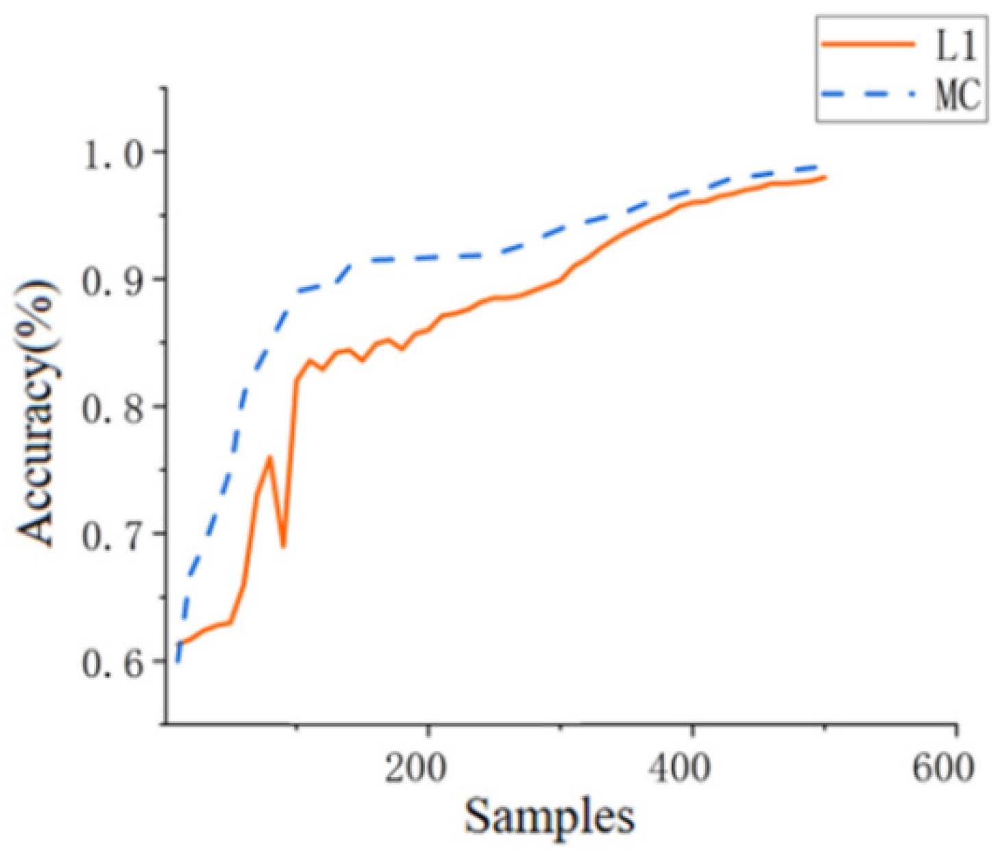
The improved primal-dual interior point method improves the iterative convergence speed of the model, and the convergence process is gentle. Compared with the original method, the new method shows good robustness, and the training process is more stable.

(3)

The simulation signals and the test analysis results from the data collected from the motorized spindle test bed and a gas turbine test bed demonstrate that this method can effectively identify the vibration and impact components in the rotor system, and provide an effective method for rotor fault diagnosis to identify the impact fault.

References

1. Sun, C.; He, Z.; Zhang, Z. Operating reliability assessment for aero-engine based on condition monitoring information. J. Mech. Eng. 2013, 49, 30–37. [Google Scholar] [CrossRef]
2. Chen, G.; Yu, M.; Liu, Y. Identifying rotor-stator rubbing positions using the cepstrum analysis technique. J. Mech. Eng. 2014, 50, 32–38. [Google Scholar] [CrossRef]
3. Amirkhani, S.; Chaibakhsh, A.; Ghaffari, A. Nonlinear robust fault diagnosis of power plant gas turbine using Monte Carlo-based adaptive threshold approach. ISA Trans. 2019, 100, 171–184. [Google Scholar] [CrossRef] [PubMed]
4. Zhao, H.; Wu, Q.; Huang, K. Status and problem research on gear study. J. Mech. Eng. 2013, 49, 11–20. [Google Scholar] [CrossRef]
5. Srivastava, A.K.; Tiwari, M.; Singh, A. Identification of rotor-stator rub and dependence of dry whip boundary on rotor parameters. Mech. Syst. Signal Process. 2021, 159, 107845. [Google Scholar] [CrossRef]
6. Kumar, A.; Tang, H.; Vashishtha, G. Noise subtraction and marginal enhanced square envelope spectrum (MESES) for the identification of bearing defects in centrifugal and axial pump. Mech. Syst. Signal Process. 2022, 165, 108366. [Google Scholar] [CrossRef]
7. Zhang, Y.; Yang, F.; Yue, H.; Deng, Z.; Xu, Y. Shock load identification of star-arrow connection and separation device based on frequency domain method. Vib. Shock 2018, 37, 79–85. [Google Scholar]
8. Le, T.; Heo, S.; Kim, H. Toward Load Identification Based on the Hilbert Transform and Sequence to Sequence Long Short-Term Memory. IEEE Trans. Smart Grid 2021, 12, 3252–3264. [Google Scholar] [CrossRef]
9. Amiri, A.K.; Bucher, C. Derivation of a new parametric impulse response matrix utilized for nodal wind load identification by response measurement. J. Sound Vib. 2015, 344, 101–113. [Google Scholar] [CrossRef]
10. Zhou, L.; Zheng, S.; Wang, B.; Lian, X.; Li, K. Transfer function coherence method for dynamic load identification position optimization. J. Vib. Eng. 2011, 24, 14–19. [Google Scholar]
11. Chen, R.; Liu, J.; Zhang, Z.; Zhang, W. A multi-source dynamic load identification method based on optimal output tracking. J. Vib. Eng. 2014, 27, 348–354. [Google Scholar]
12. Xiao, Y.; Chen, J.; Li, J. Joint denoising correction and regularization pre-optimization iteration method for time-domain identification of dynamic loads. J. Vib. Eng. 2013, 26, 52–61. [Google Scholar]
13. Qiao, B.; Chen, X.; Liu, J. Research on sparse identification method of mechanical structure impact load Chinese. J. Mech. Eng. 2019, 55, 81–89. [Google Scholar] [CrossRef]
14. Wu, Z.; Wei, Z.; Sun, L. Hyperspectral mixed pixel decomposition based on iterative weighted L1. J. Nanjing Univ. Sci. Technol. 2011, 27, 9–13. [Google Scholar]
15. Li, X.; Yu, D.; Zhang, D. Rolling bearing fault diagnosis based on resonance sparse decomposition of optimal quality factor signal. J. Vib. Eng. 2015, 28, 998–1005. [Google Scholar]
16. West, J.C.; Dixon, J.N.; Nourshamsi, N. Best Practices in Measuring the Quality Factor of a Reverberation Chamber. IEEE Trans. Electromagn. Compat. 2018, 60, 564–571. [Google Scholar] [CrossRef]
17. Chen, X.; Yu, D.; Luo, J. Envelope demodulation method based on signal resonance sparse decomposition and its application in bearing fault diagnosis. J. Vib. Eng. 2012, 25, 628–636. [Google Scholar]
18. Ouelaa, Z.; Younes, R.; Djebala, A. Comparative study between objective and subjective methods for identifying the gravity of single and multiple gear defects in case of noisy signals. Appl. Acoust. 2022, 185, 108432. [Google Scholar] [CrossRef]
19. Wang, H.; Du, W. A new K-means singular value decomposition method based on self-adaptive matching pursuit and its application in fault diagnosis of rolling bearing weak fault. Int. J. Distrib. Sens. Netw. 2020, 16, 1–12. [Google Scholar] [CrossRef]
20. Srimani, S.; Ghosh, K.; Rahaman, H. Wavelet Transform based fault diagnosis in analog circuits with SVM classifier. In Proceedings of the 2020 IEEE International Test Conference India (ITC India), Bengaluru, India, 12–14 June 2020; IEEE: New York, NY, USA. [Google Scholar]
21. Fan, W.; Li, S.; Cai, G.; Shen, C.; Huang, W.; Zhu, Z. Bearing fault diagnosis based on wavelet-based sparse signal feature extraction. Chin. J. Vib. Eng. 2015, 28, 972–980. [Google Scholar]
22. Tang, G.; Wang, X. Feature extraction of weak gear faults based on maximum correlation kurtosis deconvolution and sparse coding shrinkage. Chin. J. Vib. Eng. 2015, 28, 478–486. [Google Scholar]
23. Verbert, K.; Babuška, R.; De Schutter, B. Bayesian and Dempster-Shafer reasoning for knowledge-based fault diagnosis-A comparative study. Eng. Appl. Artif. Intell. Int. J. Intell. Real-Time Autom. 2017, 60, 136–150. [Google Scholar] [CrossRef]
24. Amin, M.T.; Khan, F.; Ahmed, S. A data-driven Bayesian network learning method for process fault diagnosis. Process Saf. Environ. Prot. 2021, 150, 110–122. [Google Scholar] [CrossRef]
25. Li, X.; Wang, J.; Zhang, B. Fault diagnosis of rolling element bearing weak fault based on sparse decomposition and broad learning network. Trans. Inst. Meas. Control 2020, 42, 169–179. [Google Scholar] [CrossRef]
26. Gajjar, S.; Kulahci, M.; Palazoglu, A. Least Squares Sparse Principal Component Analysis and Parallel Coordinates for Real-Time Process Monitoring. Ind. Eng. Chem. Res. 2020, 59, 15656–15670. [Google Scholar] [CrossRef]
27. Yan, G.; Sun, H. Research on impact load identification of composite structures based on Bayesian compressive sensing. J. Vib. Eng. 2018, 31, 483–489. [Google Scholar]
28. Mubaraali, L.; Kuppuswamy, N.; Muthukumar, R. Intelligent fault diagnosis in microprocessor systems for vibration analysis in roller bearings in whirlpool turbine generators real time processor applications. Microprocess. Microsyst. 2020, 76, 103079. [Google Scholar] [CrossRef]
29. Aster, R.C.; Borchers, B.; Thurber, C.H. Tikhonov Regularization Parameter Estimation and Inverse Problems, 2nd ed.; Elsevier: Amsterdam, The Netherlands, 2013; pp. 93–127. [Google Scholar]
30. Ngendahayo, J.P.; Niyobuhungiro, J.; Berntsson, F. Estimation of surface temperatures from interior measurements using Tikhonov regularization. Results Appl. Math. 2021, 9, 100140. [Google Scholar] [CrossRef]
31. Ravikumar, K.N.; Kumar, H.; Kumar, G.N. Fault diagnosis of internal combustion engine gearbox using vibration signals based on signal processing techniques. J. Qual. Maint. Eng. 2020; ahead-of-print. [Google Scholar]
32. Karabacak, Y.E.; Zmen, N.G.; Gümüel, L. Intelligent worm gearbox fault diagnosis under various working conditions using vibration, sound and thermal features. Appl. Acoust. 2022, 186, 108463. [Google Scholar] [CrossRef]
33. Qin, Y.; Xing, J.; Mao, Y. Weak transient fault feature extraction based on an optimized Morlet wavelet and kurtosis. Meas. Sci. Technol. 2016, 27, 085003. [Google Scholar] [CrossRef]
34. Jin, C.; Cheng, C. Two minimax theorems of mixed functions. J. Beijing Univ. Technol. 2006, 32, 269–273. [Google Scholar]
35. Zhang, Y.; Ke, W.; Lin, Q. RPSEMD based on convex optimization and its application in fault diagnosis of rolling bearings. Bearings 2020, 14, 51–57. [Google Scholar]
36. Li, S.; Wang, H.; Tang, J.; Zhang, X. Research on Fault Diagnosis of Gas Turbine Rotor Based on Adversarial Discriminative Domain Adaption Transfer Learning. Measurement 2022, 196, 111174. [Google Scholar] [CrossRef]
37. Liu, S.; Wang, H.; Zhang, X. Research on Improved Deep Convolutional Generative Adversarial Networks for Insufficient Samples of Gas Turbine Rotor System Fault Diagnosis. Appl. Sci. 2022, 12, 3606. [Google Scholar] [CrossRef]
Figure 1. Comparison of L1 norm and MC penalty.
Applsci 12 08147 g001
Figure 2. Comparison of MC penalty function curves with function (a = 1/2) curve.
Applsci 12 08147 g002
Figure 3. Process of sparse recognition method based on MC penalty function.
Applsci 12 08147 g003
Figure 4. Different sparsity parameters k robustness. (a) robustness of sparsity parameter k < 1, and (b) robustness of sparsity parameter k > 1.
Applsci 12 08147 g004
Figure 5. Accuracy changes under different input sample sizes.
Applsci 12 08147 g005
Figure 6. Time domain diagram of simulated signal. (a) time-domain diagram of no-noise, and (b) time domain diagram of noisy simulation signal.
Applsci 12 08147 g006
Figure 7. Time domain diagram of sparse decomposition results of MC.
Applsci 12 08147 g007
Figure 8. Time domain diagram of sparse decomposition results of L1.
Applsci 12 08147 g008
Figure 9. Sparse decomposition simulation amplitude/envelope results. (a) sparse decomposition amplitude spectrum, and (b) sparse decomposition envelope spectrum.
Applsci 12 08147 g009
Figure 10. The main part of the bearing vibration and impact fatigue testing machine.
Applsci 12 08147 g010
Figure 11. Donghua test acquisition analyzer.
Applsci 12 08147 g011
Figure 12. Time domain diagram of test bearing vibration signal.
Applsci 12 08147 g012
Figure 13. Time domain diagram of sparse decomposition results.
Applsci 12 08147 g013
Figure 14. Sparse decomposition simulation amplitude/envelope results. (a) sparse decomposition amplitude map, and (b) sparse decomposition envelope spectrum.
Applsci 12 08147 g014
Figure 15. Structure of a certain type of gas turbine rotor system. (1) ball bearing for low pressure compressor; (2) cylindrical roller bearing for low pressure compressor; (3) ball bearing for high pressure compressor; (4) cylindrical roller bearing for high pressure compressor; (5) cylindrical roller bearing for low pressure turbine.
Applsci 12 08147 g015
Figure 16. Time domain diagram of the original vibration signal after preprocessing.
Applsci 12 08147 g016
Figure 17. Time-domain/envelope results of sparse decomposition simulation. (a) MC penalty function sparse decomposition time domain graph, and (b) MC penalty function sparse decomposition envelope spectrogram.
Applsci 12 08147 g017
Publisher’s Note: MDPI stays neutral with regard to jurisdictional claims in published maps and institutional affiliations.