A Reinforcement Learning Method for Layout Design of Planar and Spatial Trusses using Kernel Regression

Abstract

Truss layout design aims to find the optimal layout, considering node locations, connection topology between nodes, and cross-sectional areas of connecting bars. The design process of trusses can be represented as a reinforcement learning problem by formulating the optimization task into a Markov Decision Process (MDP). The optimization variables such as node positions need to be transformed into discrete actions in this MDP; however, the common method is to uniformly discretize the design domain by generating a set of candidate actions, which brings dimension explosion problems in spatial truss design. In this paper, a reinforcement learning algorithm is proposed to deal with continuous action spaces in truss layout design problems by using kernel regression. It is a nonparametric regression way to sample the continuous action space and generalize the information about action value between sampled actions and unexplored parts of the action space. As the number of searches increases, the algorithm can gradually increase the candidate action set by appending actions of high confidence value from the continuous action space. The value correlation between actions is mapped by the Gaussian function and Euclidean distance. In this sampling strategy, a modified Confidence Upper Bound formula is proposed to evaluate the heuristics of sampled actions, including both 2D and 3D cases. The proposed algorithm was tested in various layout design problems of planar and spatial trusses. The results indicate that the proposed algorithm has a good performance in finding the truss layout with minimum weight. This implies the validity and efficiency of the established algorithm.

1. Introduction

Generative design is an intelligent design method that automatically explores and generates architectural design layouts on the premise of satisfying multiple design requirements [1]. It can be realized through structural optimization methods such as size, shape, and topology optimization [2,3,4]. As for truss structures, the optimal layout design is often represented as a combinational structural optimization problem, simultaneously considering node locations, connection topology between nodes, and cross-sectional areas of connecting bars [2]. The design variables involve both continuous and discrete types since node locations are commonly continuous variables and connections between nodes are typical discrete variables, which greatly increases the complexity of the solution space. The ground structure method first proposed by Dorn [5] is an effective and classical strategy to limit the solution space of such truss layout optimization problems and has been widely incorporated into many automatic optimization algorithms of truss layout [6,7,8,9].

The ground structure is formed by a finite number of predefined nodes and members in the design domain and the optimal truss layout can be generated by eliminating unnecessary bars and nodes in the ground structure [10]. Usually, node locations of the ground structure are uniformly sampled in the design domain; however, in order to reach a good auto-design performance, it is often necessary to discretize the design domain with a small step size. This leads to limitations in a large range of two-dimensional design domains or three-dimensional design domains for ground-structure-based methods [11]. For example, when uniformly generating nodes of the ground structure (each dimension is discretized into $k$ nodes), the number of the node candidate set is $k^2$ for two-dimensional design cases and increases to $k^3$ in three-dimensional design cases. Moreover, the total number of design variables becomes larger since the bar connections and cross-sectional areas also need to be considered. This makes the design task challenging to find the optimal truss layout [12]. The engineering design problems often need to consider constraints related to structural performance, which usually makes such optimization tasks suffer from non-convexity and non-differentiability. Many previous studies adopted search-based methods [7,9,13,14,15] to find an approximate global optimal solution instead of mathematical programming methods.

To solve such a huge solution space of the truss layout design, this optimal design task can be regarded as a decision-making problem and formulated into a Markov Decision Process (MDP) [16]. In the MDP, it is not necessary to consider all the decision variables at the same time; however, according to the decision logic of engineers, the generation of the optimal truss layout design can be gradually completed by sequential decisions [17,18]. By defining three kinds of sequential actions, which are adding nodes, adding bars, and selecting the cross-section of bars, the optimal sequence of generating actions can be obtained via Upper Confidence Trees (UCT) [19] search method, which is a reinforcement learning algorithm based on Monte Carlo Tree Search (MCTS) [20]. This UCT method has been successfully applied to the generation of planar trusses; however, there are two main problems to be solved in the generation of 3D structures by using this tree search strategy. First, the UCT algorithm also discretizes continuous variables (node location, cross-sectional area of bars); thus, the number of candidate variables increases exponentially. Although the two-stage gradual discretization strategy can be adopted, the number of variables is still a challenging problem restricting the search efficiency in 3D cases. Second, for the discretization method, the general strategy is to adopt a uniform distribution. For the UCT algorithm, if the generation interval becomes large, most discredited candidate variables are rarely utilized in the search process. This means that the neighborhood information between nodes is not fully utilized, resulting in a large amount of computing power in wasted searching.

In this paper, an algorithm KR-UCT, a UCT-based tree search method using kernel regression (KR), is proposed to solve truss layout design problems. It is applied to continuous action space and is regarded as an effective idea to estimate the reward value using the neighborhood information. The Gaussian Radial Basis Function (Gaussian Kernel) is a heuristic variables generation strategy to deal with continuous variables, which reflects the neighborhood information of the search region. For the truss generation problem, continuous variables such as node coordinates and bar sectional area have a good neighborhood correlation during the tree search process. Gaussian Kernel function can progressively widen the search tree, so as to improve the quality of each decision and the UCT search efficiency by reducing the size of action sets.

2. Reinforcement Learning Task for Truss Layout Design

2.1. Problem Statement

Truss optimal layout design problems involve three kinds of optimization aspects: topology, shape, and size, aiming to find the optimal node positions, bar connections, and bar sectional areas, respectively. This optimal design is usually aimed at finding the layout with the minimum structural weight under linear and nonlinear constraints that limit design variable range, such as structural performance and other design requirements. To make this design task clear, the constraints used in this paper are listed in

Table 1. Constraints used in this paper.

Constraints		Expression
$g_1$	Design domain, $\mathsf{\Omega }$	Check element position in $\mathsf{\Omega }$
$g_2$	Cross-sectional area	$A_{min}\le A_i\le A_{max}$
$g_3$	Strength	$-{\sigma }_{min}\le {\sigma }_i\le {\sigma }_{max}$
$g_4$	Displacement	${\delta }_j\le {\delta }_{max}$
$g_5$	Stability	${\sigma }_i^c\le {\sigma }_{buckle}$
$g_6$	Stiffness	${\lambda }_i\le {\lambda }_{max}$
$g_7$	Bar length	$l_{min}\le l_i\le l_{max}$

, which can be seen as a set to form different constraint combinations $G$ in different experiments. Thus, the layout design problems involved in this paper can be expressed as:

$$minimize W\left(P,E\right)={\displaystyle \sum }_i\rho l_i{A}_i,$$

(1)

$$subjected to G=\left\{G|G\in \left\{g_1,g_2,g_3,g_4,g_5,g_6,g_7\right\}\right\},$$

(2)

where $W\left(P,E\right)$ is the weight of the structure, $P,$ and $E$ are the node set and the edge set of the structure, $\rho$ is the material density, $l_i$ and $A_i$ are the length and cross-sectional area of the $i^{th}$ bar. ${\sigma }_i$ is the stress of $i^{th}$ bar; ${\delta }_j$ is maximum displacement in all directions of the $j^{th}$ node; ${\sigma }_i^c$ is the stress of the $i^{th}$ bar in compression, in general, ${\sigma }_{buckle}={\pi }^{2}E{I}_i/(A_i{l}_i^2)$, where $I_i$ is the moment of inertia of the $i^{th}$ bar; ${\lambda }_i$ is the slenderness ratio of the $i^{th}$ bar. The subscripts $min$ and $max$ represent the upper and lower bound of the corresponding variable, respectively.

For constraint $g_1$, the design domain $\mathsf{\Omega }$ defines the boundaries for the position of the truss element [21]. Constraint $g_2$ defines the upper and lower bounds for the cross-sectional area of bars. For constraint $g_3$, the stress of each truss member should be lower than the allowable stress [9]. The displacement constraint $g_4$ is formulated by considering that the nodal displacement must be lower than the allowable displacement [22]. Constraint $g_5$ represents the buckling instability of the bar. All bar sections used in this paper are circular solid sections unless otherwise stated [23]. Constraints $g_6$ and $g_7$ define the limits of slenderness ratio and length of bars, respectively.

Note that the search-based method is a kind of “black box” optimization model; the algorithm is applicable for different objectives. Here, the most common objective, the minimum weight, is selected as the model objective for the convenience of comparing the experimental results with other literature. The design domain Ω and specific load case information will be given in the specific experiment.

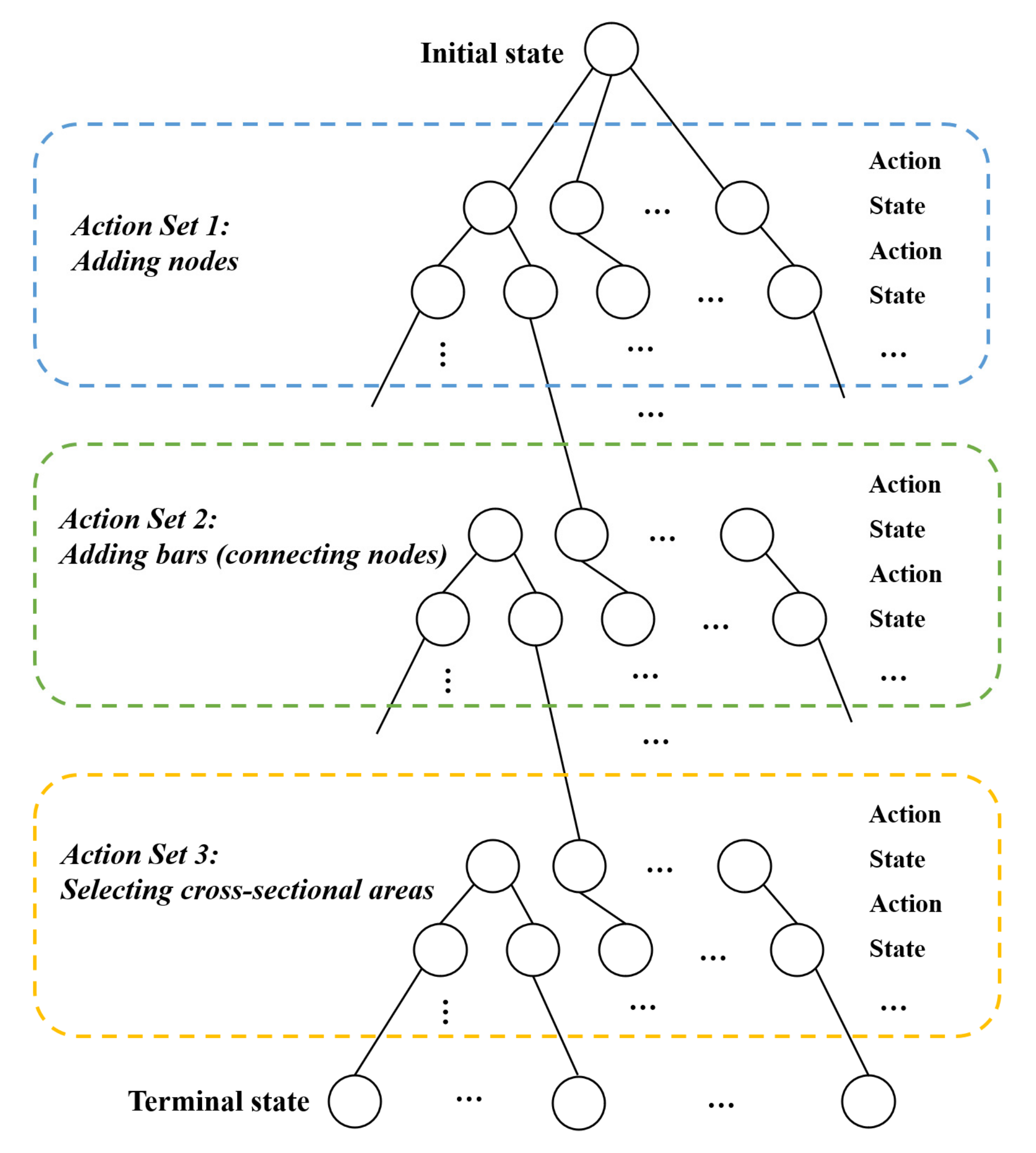
2.2. Sequential Decision Model for Truss Layout Design

Markov Decision Processes (MDP) is the most basic theoretical model and mathematical expression for Reinforcement Learning problems [24]. The purpose of MDP is to construct a classical formal expression of sequential decision problems, which can construct an interactive learning model between an agent and the environment. The design process of truss layout can be modeled as an MDP model, which contains four components: state, action, transition model, and reward. A state can be expressed as all the information possessed by the current truss layout. When reaching a state that is not terminated, the agent will take a corresponding action by observing the characteristics of the state. The action contains three sequential types, that is, adding nodes, adding bars, and selecting cross-sectional areas of the bars. After taking an action, the transition model indicates the probability distribution of the next state. When all the decision steps have been completed, the agent will calculate a numerical reward based on the objective. The reward can guide the algorithm in the right searching direction towards a better solution. The details of the reward function are given in the pseudo-code Algorithm 1.

Algorithm 1 Mixed reward function for evaluation
	Input: Node Set $P$, Bar Set $E$, Current iteration $iter$  Output: Reward of Structure $\left(P,E\right)$
1:	Function$Reward\left(P, E\right)$ //feedback signal to the agent
2:	If $IsStructure\left(P, E\right)$ then
3:	$obj\leftarrow$ objective of $\left(P,E\right)$
4:	If $iter<i_{mark}$
5:	Return $f{\left(obj\right)}_{soft}$
6:	For every constraint $c$ do
7:	If $\left(P, E\right)$ does not pass $c$ then
8:	Return $0$
9:	End For
10:	Return $f{\left(obj\right)}_{hard}$
11:	Return$-1$
12:
13:	Function$IsStructure\left(P, E\right)$ //check geometry stability
14:	$d\leftarrow$ dimension of $\left(P, E\right)$
15:	$r\leftarrow$ number of restricted degrees of freedom at support nodes of $\left(P, E\right)$
16:	$N\leftarrow d\times \left|P\right|-\left|E\right|-r$
17:	If $N\le 0$ then
18:	$K\leftarrow$ stiffness matrix of $\left(P, E\right)$
19:	If $K\succ 0$ then
20:	Return True
21:	Return False

First, the reward function checks the geometric stability of the generated truss. The check process is performed by the function IsStructure. The checking process is divided into two steps: firstly, the Degree of Freedom (DOF) of the generated truss is calculated according to the Maxwell criterion [25]. If $DOF>0$, a negative reward -1 will be passed on to the agent. If $DOF\le 0$, evaluate the positive definiteness of the stiffness matrix of the truss. If the generated truss is judged as a mechanism by stiffness matrix evaluation, a negative reward of -1 will also be passed on to the agent as a penalty.

When the generated truss passes the IsStructure function, the algorithm returns a nonnegative reward to the agent according to the iteration number and the structural performance of the current layout. Specifically, if $iteration<i_{mark}$, the reward is calculated by $f{\left(obj\right)}_{soft}$. Otherwise, the reward is directly assigned as $f{\left(obj\right)}_{hard}$. $f{\left(obj\right)}_{soft}$ is a soft reward model and gives punishment when existing constraint violations. The expression of the soft reward model can be defined as follows:

$$f{\left(obj\right)}_{soft}=\frac{\lambda }{W{\left(P,E\right)}^2*\left(1+\sum penalt{y}_{g_i} \right)}$$

(3)

In Equation (3), $penalt{y}_{g_i}$ is the percentage of constraint violations and $\lambda$ is a parameter to standardize the reward value according to different experiments. $f{\left(obj\right)}_{hard}$ is a hard reward model and only gives positive reward value to those layouts that pass all the constraints; otherwise, the agent will only receive a zero reward. The expression of the hard reward model can be defined as follows:

$$f{\left(obj\right)}_{hard}=\frac{\lambda }{W{\left(P,E\right)}^2}$$

(4)

3. Methodology for Model Solving

3.1. Monte Carlo Tree Search for Truss Layout Design

Monte Carlo Tree Search (MCTS) [19,26] is a reinforcement learning algorithm for selecting the optimal action of a Markov Decision Process (MDP). Starting from an empty tree, the algorithm iteratively expands the search three through a loop consisting of four steps, naming selection, expansion, simulation, and backpropagation. For optimal layout design of trusses, the generation process was first formulated into an MDP and an algorithm based on MCTS [20]. The algorithm is referred to as UCT using the improved upper confidence bounds in the search tree. Given initial loads and supports conditions, a planar truss layout can be generated through the truss layout MDP with three sequential action sets. The whole decision process represented by the search tree is shown in Figure 1.

Firstly, the UCT algorithm adds nodes into the structure. After that, it adds bars between the existing nodes. Finally, the cross-sectional area of each bar is selected. The authors applied adjustments to MCTS for adapting the algorithm to the optimal design task, evaluating the upper confidence bound of state $j$ using

$$U_j=\alpha \times {\overline{v}}_j+\left(1-\alpha \right)\times vbes{t}_j+C\times \sqrt{\frac{\ln \left({{\displaystyle \sum }}_k{n}_k\right)}{n_j}}$$

(5)

where, ${\overline{v}}_j$ is the average reward; $vbes{t}_j$ is the optimal best reward; the parameter α is used to adjust the proportion of the optimal best reward; $n_j$ is the number of simulations. Usually, C is set as a positive constant, keeping $U_j=+\infty$ when $n_j=0$.

3.2. Kernel Regression UCT for Truss Layout Design

The UCT algorithm has been proven to be effective for truss generation [20]; however, there remains a problem dealing with continuous action space. Notice that the coordinates of newly added nodes and cross-sectional areas of bars are often continuous variables. The strategy for uniformly discretizing the continuous decision space would cause exponential growth of candidate nodes in 3D cases; therefore, it is worth looking for some method to discretize the action space while controlling the size of candidate sets and the value of each action in the collection. That is, a continuous action set, which is of finite size and heuristically generated, is required.

To control the size of the candidate set, one direct approach is to gradually expand the width of the search tree as the number of loop iteration grows. More concretely, the $n$th candidate action is added to the search tree after $T\left(n\right)$ loops of MCTS have proceeded. This approach was independently introduced in [27] named progressive widening. Commonly, $T\left(n\right)$ can be set to a power function. In this paper, $T\left(n\right)$ is set to be $3n^2$.

When adding a new action to the candidate set, the previous search information should be considered to give a reference for choosing high-value candidate actions. This paper uses the Gaussian Radial Basis Function [28] to evaluate the neighborhood information, which is a nonparametric fit to the existing search experience. More concretely, when sampling an action with a continuous variable vector $\overrightarrow{\mathit{x}}$ once, another action $\overrightarrow{\mathit{y}}$ is treated to be sampled

$$K\left(\overrightarrow{\mathit{x}}, \overrightarrow{\mathit{y}}\right)= \exp \left(-\frac{\Vert \overrightarrow{\mathit{x}}-{\overrightarrow{\mathit{y}}\Vert }^2}{2{\sigma }^2}\right)$$

(6)

times. Assume $m$ simulations are processed, vector ${\overrightarrow{\mathit{x}}}_i$ is sampled with a reward of $r_i$ in $i$th simulation and the vector ${\overrightarrow{\mathit{x}}}_i$ is sampled $n_{{\overrightarrow{\mathit{x}}}_i}$ times. For an action vector $\overrightarrow{\mathit{y}}$, the weighting function can be defined as

$$W\left(\overrightarrow{\mathit{y}}\right)={\displaystyle \sum }_{i=1}^{m}K\left({\overrightarrow{\mathit{x}}}_i, \overrightarrow{\mathit{y}}\right)n_{{\overrightarrow{\mathit{x}}}_i}.$$

(7)

Similarly, the average reward of an action vector $\overrightarrow{\mathit{y}}$ can be approximately evaluated by

$$\overline{v}\left(\overrightarrow{\mathit{y}}\right)=\frac{W\left(\overrightarrow{\mathit{y}}\right)r_i}{W\left(\overrightarrow{\mathit{y}}\right)}=\frac{{{\displaystyle \sum }}_{i=1}^{m}K\left({\overrightarrow{\mathit{x}}}_i, \overrightarrow{\mathit{y}}\right)n_{{\overrightarrow{\mathit{x}}}_i}{r}_i}{{{\displaystyle \sum }}_{i=1}^{m}K\left({\overrightarrow{\mathit{x}}}_i, \overrightarrow{\mathit{y}}\right)n_{{\overrightarrow{\mathit{x}}}_i}}$$

(8)

using Equations (7) and (8), the adjusted upper confidence bound in our approach can be written as

$$U_{\overrightarrow{\mathit{y}}}=\alpha \times \overline{v}\left(\overrightarrow{\mathit{y}}\right)+\left(1-\alpha \right)\times vbes{t}_{\overrightarrow{\mathit{y}}}+C\times \sqrt{\frac{\ln \left({{\displaystyle \sum }}_{\overrightarrow{\mathit{x}}}W(\overrightarrow{\mathit{x}})\right)}{W\left(\overrightarrow{\mathit{y}}\right)}}$$

(9)

Notice that the constraints in the generation process are strict, indicating that a small difference in node position or bar area may let the structure fail to pass a constraint. Therefore, the optimal structure found by the algorithm cannot be evaluated around the neighborhood. When $\overrightarrow{\mathit{y}}$ has not been simulated, $vbes{t}_{\overrightarrow{\mathit{y}}}$ is initially set to 0.

The selection strategy of a new action should discover the unknown area of the continuous space with a high expected reward. To discover the unknown area, the weight function of the new action should be small. To keep a high expected reward, assume the current optimal action is $\overrightarrow{\mathit{y}}$, the new action should be chosen from the neighbor of $\overrightarrow{\mathit{a}}$; therefore, the new action is chosen by

$${\mathrm{argmin} }_{||\overrightarrow{\mathit{a}}-\overrightarrow{\mathit{y}}||<\tau } W\left(\overrightarrow{\mathit{a}}\right)$$

(10)

Notice that the optimization above is hard to compute, so we approximate it by selecting the action with minimum weight function from $k$ actions randomly generated from the space $||\overrightarrow{\mathit{a}}-\overrightarrow{\mathit{y}}||<\tau$.

A truss generation algorithm with a continuous variable selection strategy is well defined after applying the progressive widening method with the approximation strategy mentioned above to the first and the third stage of the UCT algorithm introduced in Section 2.2. This approach uses the kernel regression function to approximately evaluate the neighborhood; the abbreviation KR-UCT refers to this approach in the following text. For a more detailed version, the pseudo-code of this approach is shown in Algorithm 2.

Algorithm 2 KR-UCT Algorithm for Truss Generation
	Input: Node Set $P$, Bar Set $E$, Allowed Area Interval $I_A$, Number of Nodes $maxp$, Design Envelope $D$  Output: Generated Node Set $P_{opt}$, Generated Bar Set $E_{opt}$
1:	$A\leftarrow InitialSet\left(P,E\right)$ //generate initial available action set
2:	While$ActionSet\left(P,E\right)\ne \varnothing$do
3:	$a^{*}\leftarrow KRTreeSearch\left(P,E\right)$ //the beat action $a^{*}$ in the state (P, E)
4:	$P,E\leftarrow TakeAction\left(P,E,a^{*}\right)$ //allpy action $a^{*}$ to update state $\left(P,E\right)$
5:	End While
6:	$P_{opt}, E_{opt}\leftarrow P,E$
7:	Return$P_{opt}, E_{opt}$ //obtain the optimal truss layout
8:
9:	$A\leftarrow InitialSet\left(P,E\right)$ //generate initial available action set
10:	$opt\leftarrow ActionSet\left(P,E\right)$
11:	If $opt=1$ then
12:	$A\leftarrow$ add new candidate points $x_i| i=1\dots n_{init}$, $x_i$ is randomly sampled //node location $x_i$ is a multidimensional vector
13:	If $opt=2$ then
14:	$A\leftarrow$ add a bar from all allowed bars
15:	If $opt=3$ then
16:	$id\leftarrow$index of the first unmodified bar
17:	$A\leftarrow$ modify the area of $E_{id}$ to $a_i | i=1\dots n_{init}$, $a_i$is randomly sampled //cross-sectional area $a_i$ a one-dimensional vector (scalar).
18:	Return $A$
19:
20:	Function$ActionSet\left(P,E\right)$ //Returns the action type corresponding to the current state
21:	If $\left|P\right|<Np$ then
22:	Return $1$ //action set 1: add nodes
23:	If $Reward\left(P, E\right)\le 0$ then
24:	Return $2$ //action set 2: add bars connections
25:	$id\leftarrow$ index of the first unmodified bar
26:	If $id$ exits then
27:	Return $3$ //action set 3: modify the area of the bars
28:	Return $\varnothing$
29:
30:	Function$KRTreeSearch\left(P,E\right)$//tree search algorithm
31:	For $iter=0$ to $Maxiter$ do
32:	$P_{new},E_{new}\leftarrow P, E$
33:	While $\left(P_{new}, E_{new}\right)$ in Tree and $ActionSet\left(P_{new},E_{new}\right)\ne \varnothing$ do//selection
34:	$opt\leftarrow ActionSet\left(P_{new}, E_{new}\right)$ //tree policy
35:	If $opt=1$ then
36:	$act \leftarrow arg{\max }_{x_i\in A_{now}} U_{x_i}$ //$U_{x_i}$ is defined in Equation (9)
37:	If ${{\displaystyle \sum }}_{x_i\in A_{now}}{n}_{x_i}>3\times {\left|A_{now}\right|}^2$ then //progressive widening
38:	$x_{new}\leftarrow { \mathrm{argmin} }_{\left|\left|x_{new}-act\right|\right|<\tau } W\left(x_{new}\right)$ //see Equation (10)
39:	$act \leftarrow add x_{new} into P$
40:	$A_{now} \leftarrow A_{now} \cup act$
41:	If $opt=2$ then
42:	$act\leftarrow arg{\max }_{a\in A_{now}}{v}_a+C\sqrt{\frac{\ln \left({{\displaystyle \sum }}_{b\in A_{now}}{n}_b\right)}{n_a}}$
43:	If $opt=3$ then
44:	$act \leftarrow arg{\max }_{x_i\in A_{now}} U_{a_i}//U_{a_i}$ is defined in Equation (9)
45:	If ${{\displaystyle \sum }}_{a_i\in A_{now}}{n}_{a_i}>3\times {\left|A_{now}\right|}^2$ then //progressive widening
46:	$a_{new}\leftarrow { \mathrm{argmin} }_{a_{new}-act<\tau } W\left(a_{new}\right)$ //see Equation (10)
47:	$act \leftarrow$modify the area of the current bar to $a_{new}$
48:	$A_{now} \leftarrow A_{now} \cup act$
49:	$\left(P_{new}, E_{new}\right)\leftarrow TakeAction\left(P_{new}, E_{new},act\right)$
50:	End While
51:	If $\left(P_{new}, E_{new}\right)$ is not in the search tree then //expand
52:	$Expand\left(P_{new}, E_{new}\right)$
53:	$P_{tmp}, E_{tmp}\leftarrow P_{new},E_{new}$
54:	While $ActionSet\left(P_{tmp},E_{tmp}\right)=\varnothing$ do //default policy
55:	$P_{tmp}, E_{tmp}\leftarrow TakeAction\left(P_{tmp}, E_{tmp}, a_{random}~A_{tmp}\right)$
56:	End While
57:	$r=Reward\left(P_{tmp},E_{tmp}\right)$ //simulation
58:	While $(P_{new},E_{new}) \ne \left(P, E\right)$ do //backpropagation
59:	use $r$ to update all related values of $(P_{new}, E_{new})$
60:	$(P_{new},E_{new})\leftarrow fa\left(P_{new},E_{new}\right)$
61:	End While

3.3. Modification for Symmetry Truss Layout Design

To develop designs that are topologically unique and interesting, and yet somewhat regular for practical and constructability considerations, global constraints such as symmetry can be enforced before the design generation. For KR-UCT, the operation objects are the most basic structural units: node, bar, and cross-sectional area. Thus, the design adapted to specific geometric constraints can be generated by modifying the truss generation process. The main idea of the modification is to do all actions symmetrically.

For the add-node step, there are two kinds of ways to add nodes. The first way is to add one node if this node is on the vertical symmetry axis of the design domain. Note that the axis of symmetry mentioned below all refers to the vertical symmetry axis of the design domain. The second way is to add two symmetric nodes at the same time and regard it as one add-node action. For the add-bar step, there are two kinds of ways to add bars. The first way is to add one bar if this bar is originally symmetrical in the layout. The second way is to add two symmetric bars at the same time, which can be regarded as one action. The final step is to modify the cross-sectional area of bars according to the adding order in the second step. The only difference in this step is to simultaneously modify the area of two symmetric bars if they are added by the second way of the add-bar step.

4. Numerical Experiments

4.1. Proof of Concept

As mentioned, the most significant difference between UCT and KR-UCT is whether the design variables are continuous values or not. Serving as a proof of concept, the 17-bar truss experiment is used to demonstrate the design workflow of the KR-UCT algorithm. This experiment illustrates the design of a long cantilever truss in the design domain. The design domain of the 17-bar truss and the details of specified essential nodes [21] are shown in Figure 2 and

Table 2. Essential node coordinates in the 17-bar experiment.

Essential Node	Node Location (mm)	Node Label
$\left(1\right)$	$\left(0, 0\right)$	$\mathrm{Pinned} \mathrm{support}$
$\left(2\right)$	$\left(0, 2540\right)$	$\mathrm{Pinned} \mathrm{support}$
$\left(3\right)$	$\left(10,160, 0\right)$	$\mathrm{Loading}$ (0, −444,800 N)

. The settings of material properties are given in

Table 3. Material property settings in the 17-bar experiment.

Material Properties	Settings
$\mathrm{Young}’\mathrm{s} \mathrm{modulus}$	206,850 MPa
$\mathrm{Density}$	$7418.21 \mathrm{kg}/{\mathrm{m}}^3$

. The constraint combination in this experiment is $\left(g_1,g_2,g_3,g_4,g_5\right)$, and the parameters or formulas are summarized in

Table 4. Constraint parameter settings in the 17-bar experiment.

Constraints	Parameters	Settings
${\mathrm{g}}_1$	Xmin; Xmax Ymin; Ymax	$0 \mathrm{mm};10,160 \mathrm{mm};$ $0 \mathrm{mm};2540 \mathrm{mm}$
${\mathrm{g}}_2$	${\mathrm{A}}_{\min },{\mathrm{A}}_{\max }$	$0.6452 {\mathrm{cm}}^2;200 {\mathrm{cm}}^2$
${\mathrm{g}}_3$	${\mathsf{\sigma }}_{\min },{\mathsf{\sigma }}_{\max }$	$334.6 \mathrm{MPa};334.6 \mathrm{MPa}$
${\mathrm{g}}_4$	${\mathsf{\delta }}_{\max }$	$50.8 \mathrm{mm}$
${\mathrm{g}}_5$	${\mathsf{\sigma }}_{\mathrm{buckle}}$	${\mathsf{\pi }}^2\mathrm{EI}/{\mathrm{L}}^2$

. The purpose of this experiment was to find the truss layout of minimum weight under constraints.

There are three action sets for KR-UCT to choose sequentially. In the first action set, nodes are chosen from the candidate node set and added to the structure. In UCT, the design domain needs to be uniformly discretized, whereas, in KR-UCT, only the initial number of actions needs to be set. All initial actions are generated randomly from the design domain. In the second action set, several bars are added to the truss until it passes all the constraints. In the third action set, KR-UCT assigns optimal cross-sectional areas to the generated bars. In UCT, the candidate cross-sectional area set ($\left[A_{\min },A_{\max }\right]$), also needs to be discretized. In KR-UCT, only the initial number of actions needs to be set. All initial actions are generated randomly from the optional cross-sectional area set.

Figure 3 shows the optimal truss layout in this experiment. The weight of the optimal truss layout is 1463.44 kg. Note that a bar in red/blue color indicates that it is in tension/compression, respectively. Figure 4 shows its construction process, which depicts how KR-UCT makes decisions to build a truss. In the UCT algorithm, the node candidate set in every step of the adding-node stage is uniformly discretized, as shown in Figure 5; Figure 6 shows the heuristic distribution of node candidate sets in the KR-UCT algorithm in order to prove the effectiveness of kernel regression. It is found that, in each step of adding a node to the truss, a large number of optional actions are gathered around the location of the final selected point. This indicates that the selection of optional node location has heuristic significance.

To verify the effectiveness of the KR-UCT algorithm, the optimal solution of KR-UCT is compared with that of UCT. The comparison results are shown in

Table 5. Comparison results of the 17-bar experiment.

Algorithm	UCT [20]	KR-UCT
$\mathrm{weight} \left(\mathrm{kg}\right)$	$1695.89$	$1463.44$

. The optimal solution found in this study weighs 1463.44 kg, which is about 13.7% lighter and topologically different from the one generated by the UCT algorithm.

4.2. 10-Bar Planar Truss Experiment

To further verify the effectiveness of the KR-UCT algorithm, another comparison with the UCT algorithm is carried out under the same design domain, constraints, and load cases for the 10-bar planar truss experiment. The design domain is shown in Figure 7 and the details of specified essential nodes are given in

Table 6. Essential node coordinates in the 10-bar experiment.

Essential Node	Node Location (mm)	Node Label
$\left(1\right)$	$\left(0, 0\right)$	$\mathrm{Pinned} \mathrm{support}$
$\left(2\right)$	$\left(0, 9144\right)$	$\mathrm{Pinned} \mathrm{support}$
$\left(3\right)$	$\left(9144, 0\right)$	$\mathrm{Loading} \left(0,-\mathrm{444,800} \mathrm{N}\right)$
$\left(4\right)$	$\left(\mathrm{18,288}, 0\right)$	$\mathrm{Loading} \left(0,-\mathrm{444,800} \mathrm{N}\right)$

. Material property settings are summarized in

Table 7. Material property settings in the 10-bar experiment.

Material Properties	Settings
$\mathrm{Young}’\mathrm{s} \mathrm{modulus}$	$\mathrm{68,950} \mathrm{MPa}$
$\mathrm{Density}$	$2767.99 \mathrm{kg}/{\mathrm{m}}^3$

. The constraint combination in this experiment is $\left(g_1,g_2,g_3,g_4,g_5\right)$, and the parameters or formulas are given in

Table 8. Constraint parameter settings in the 10-bar experiment.

Constraints	Parameters	Settings
${\mathrm{g}}_1$	Xmin; Xmax Ymin; Ymax	0 mm; 18,288 mm $0 \mathrm{mm};9144 \mathrm{mm}$
${\mathrm{g}}_2$	${\mathrm{A}}_{\min };{\mathrm{A}}_{\max }$	$0.6452 {\mathrm{cm}}^2;400 {\mathrm{cm}}^2$
${\mathrm{g}}_3$	${\mathsf{\sigma }}_{\min };{\mathsf{\sigma }}_{\max }$	$172.3 \mathrm{MPa};172.3 \mathrm{MPa}$
${\mathrm{g}}_4$	${\mathsf{\delta }}_{\max }$	$50.8 \mathrm{mm}$
${\mathrm{g}}_5$	${\mathsf{\sigma }}_{\mathrm{buckle}}$	${\mathsf{\pi }}^2\mathrm{EI}/({\mathrm{Al}}^2)$

. The goal of this experiment is to find the truss layout of minimum weight under constraints.

In order to make the comparison in a more detailed manner, this paper uses a series of node number settings (maxp) varying from 6 to 9. The comparison results are summarized in

Table 9. Minimum weights (kg) for the different number of nodes in the 10-bar planar truss experiment.

Algorithms		Assimi et al. [9]	Fenton et al. [21]	UCT [20]	KR-UCT
Number of nodes (maxp)	6	2223.5	2217.54	2223.10	2153.87
	7	N/A	N/A	2255.72	1968.72
	8	N/A	N/A	2280.93	1852.46
	9	N/A	N/A	2339.62	2122.05

. The generative design results are shown in Figure 8.

In the structural design practice, the global optimal and unique solution does not always satisfy the architects’ design intuition. Usually, they need a variety of different designs with high structural performance. The proposed algorithm has the ability to generate multiple competitive solutions with significantly different layouts. In KR-UCT, the three types of action in the decision-making process can expand the solution space. Note that each decision trajectory does not affect the other. This can fully explore the solution space and ensure the independence of every decision trajectory. Further, the Monte Carlo method can bring randomness to action-making steps in the decision tree; therefore, KR-UCT can generate various competitive truss design solutions under the same design requirements (design objectives, constraints, algorithm parameters). Figure 9 shows several truss layouts obtained by the KR-UCT algorithm when the total number of nodes is set to 8. The 12 layouts illustrated in Figure 9 have a weight ranging from 1852.46 kg to 2306.61 kg.

4.3. 39-Bar Planar Truss Experiment

The task of this experiment is the generation of a planar simply supported truss in the design domain, as shown in Figure 10. The details of specified essential nodes and material property settings are summarized in

Table 10. Essential node coordinates in the 39-bar experiment.

Essential Node	Node Location (mm)	Node Label
$\left(1\right)$	$\left(0, 0\right)$	$\mathrm{Pinned} \mathrm{support}$
$\left(2\right)$	$\left(\mathrm{12,192}, 0\right)$	$\mathrm{Sliding} \mathrm{support}$
$\left(3\right)$	$\left(3048, 0\right)$	$\mathrm{Loading} \left(0,-\mathrm{88,964} \mathrm{N}\right)$
$\left(4\right)$	$\left(9144, 0\right)$	$\mathrm{Loading} \left(0,-\mathrm{88,964} \mathrm{N}\right)$
$\left(5\right)$	$\left(6096, 0\right)$	$\mathrm{Loading} \left(0,-\mathrm{88,964} \mathrm{N}\right)$

and

Table 11. Material property settings in the 39-bar experiment.

Material Properties	Settings
$\mathrm{Young}’\mathrm{s} \mathrm{modulus}$	$68,950 \mathrm{MPa}$
$\mathrm{Density}$	$2767.99 \mathrm{kg}/{\mathrm{m}}^3$

. The constraint combination used in this experiment is $\left(g_1,g_2,g_3,g_4\right)$ and the parameters are given in

Table 12. Constraint parameter settings in the 39-bar experiment.

Constraints	Parameters	Settings
${\mathrm{g}}_1$	Xmin; Xmax Ymin; Ymax	$0 \mathrm{mm};\mathrm{12,192} \mathrm{mm};$ $0 \mathrm{mm};6096 \mathrm{mm}$
${\mathrm{g}}_2$	${\mathrm{A}}_{\min };{\mathrm{A}}_{\max }$	$0.323 {\mathrm{cm}}^2;14.516 {\mathrm{cm}}^2$
${\mathrm{g}}_3$	${\mathsf{\sigma }}_{\min };{\mathsf{\sigma }}_{\max }$	$137.9 \mathrm{MPa};137.9 \mathrm{MPa}$
${\mathrm{g}}_4$	${\mathsf{\delta }}_{\max }$	$50.8 \mathrm{mm}$

. The purpose of this experiment is to find the truss layout of minimum weight under given constraints.

Figure 11 depicts the optimal truss layout generated for this experiment. In this experiment, the third step of KR-UCT can be simplified because this problem is controlled by stress constraints. Hence, the structural optimization criterion, i.e., the full stress criterion [29], can help the agent to make the selection of cross-sectional area faster and better. The third step of KR-UCT is no longer to adjust the cross-section of bars but to give all bars the cross-section directly according to the fully stressed design criterion.

The optimal solution of KR-UCT is compared with that from other literature, as shown in

Table 13. Comparison results of the 39-bar experiment.

Algorithm	GA [30]	AS-API [31]	AMPDE [32]	FA [22]	IPVS [7]	KR-UCT
$\mathrm{weight}\left(\mathrm{kg}\right)$	$87.18$	$85.61$	$85.48$	$86.77$	$84.30$	$82.14$

. The optimal solution found in this study weighs 82.14 kg, which is about 2.56% lighter than the IPVS algorithm [7]. It should be noted that by introducing symmetry, the number of decision steps required to generate this truss structure is reduced from 49 to 26, which reduces the total decision length by nearly half. Thus, the decision process can be significantly shortened by introducing symmetry into the actions of MDP.

4.4. Long-Span Truss Bridge Experiment

This section presents an experiment with more kinds of constraints. All constraints are set according to AISC design specifications [33], which makes this experiment closer to engineering practice. The design domain of this long-span bridge is given in Figure 12. The details of specified essential nodes and material property settings are shown in

Table 14. Essential node coordinates in the long-span bridge experiment.

Essential Node	Node Location (mm)	Node Label
$\left(1\right)$	$\left(0, 0\right)$	$\mathrm{Pinned} \mathrm{support}$
$\left(2\right)$	$\left(\mathrm{70,000}, 0\right)$	$\mathrm{Sliding} \mathrm{support}$
$\left(3\right)$	$\left(\mathrm{10,000}, 0\right)$	$\mathrm{Loading}\left(0,-\mathrm{500,000} \mathrm{N}\right)$
$\left(4\right)$	$\left(\mathrm{60,000}, 0\right)$	$\mathrm{Loading}\left(0,-\mathrm{500,000} \mathrm{N}\right)$
$\left(5\right)$	$\left(\mathrm{20,000}, 0\right)$	$\mathrm{Loading}\left(0,-\mathrm{500,000} \mathrm{N}\right)$
$\left(6\right)$	$\left(\mathrm{50,000}, 0\right)$	$\mathrm{Loading}\left(0,-\mathrm{500,000} \mathrm{N}\right)$
$\left(7\right)$	$\left(\mathrm{30,000}, 0\right)$	$\mathrm{Loading}\left(0,-\mathrm{500,000} \mathrm{N}\right)$
$\left(8\right)$	$\left(\mathrm{40,000}, 0\right)$	$\mathrm{Loading}\left(0,-\mathrm{500,000} \mathrm{N}\right)$

and

Table 15. Material property settings in the long-span bridge experiment.

Material Properties	Settings
$\mathrm{Young}’\mathrm{s} \mathrm{modulus}$	$201 \mathrm{GPa}$
$\mathrm{Density}$	$7851.03 \mathrm{kg}/{\mathrm{m}}^3$
$\mathrm{Yield} \mathrm{strength}$	$248.8 \mathrm{MPa}$

. The constraint combination in this experiment is $(g_1,g_2,g_3,g_4,g_6,g_7$). Two relevant AISC design specifications are given as follows. First, the allowable tension stress ${\sigma }_t$ of bars is 0.6$f_y$. Second, the allowable compression stress ${\sigma }_c$ is computed by Equation (11):

$${[\sigma ]}_C=\left\{\begin{array}{ll}\frac{12{\pi }^{2}E}{23{\lambda }^2},& if {\lambda }_j>C\\ \frac{\left(1-\frac{{\lambda }^2}{2C^2}\right)f_y}{\frac{5}{3}+\frac{3\lambda }{8C}-\frac{{\lambda }^3}{8C^3}}, & if {\lambda }_j<C \end{array}\right.,$$

(11)

where $\lambda =L/r$, $C=\pi \sqrt{2E/f_y}$, and $L$ and r are the length and radius of gyration of the cross-section of bars; the allowable node displacement is limited to $1/1000$ of span, i.e., 70 mm; the allowable bar slenderness ratios are specified to be 300 for tension bars and 200 for compression bars; the minimum and minimum length of bars are 5 m and 35 m, respectively. Note that all the truss bars are selected from a set of 30 standard AISC sections, i.e., $\mathrm{W}14\times 22$ through $\mathrm{W}14\times 426$. The purpose of this experiment is to find the truss layout of minimum weight under given constraints.

Figure 13 illustrates the optimal truss layout generated for this experiment. The optimal solution of KR-UCT is compared with those obtained from other literature. The comparison results are given in

Table 16. Comparison results of the long-span bridge truss experiment.

Algorithm	GA [35]	GP [34]	GA [36]	KR-UCT
$\mathrm{weight}\left(\mathrm{kg}\right)$	$\mathrm{60,329}$	$\mathrm{45,404}$	$\mathrm{46,222}$	$\mathrm{44,566}$

. The optimal solution found in this study weighs 44,566 kg, which is about 1.85% lighter than the GP algorithm [34].

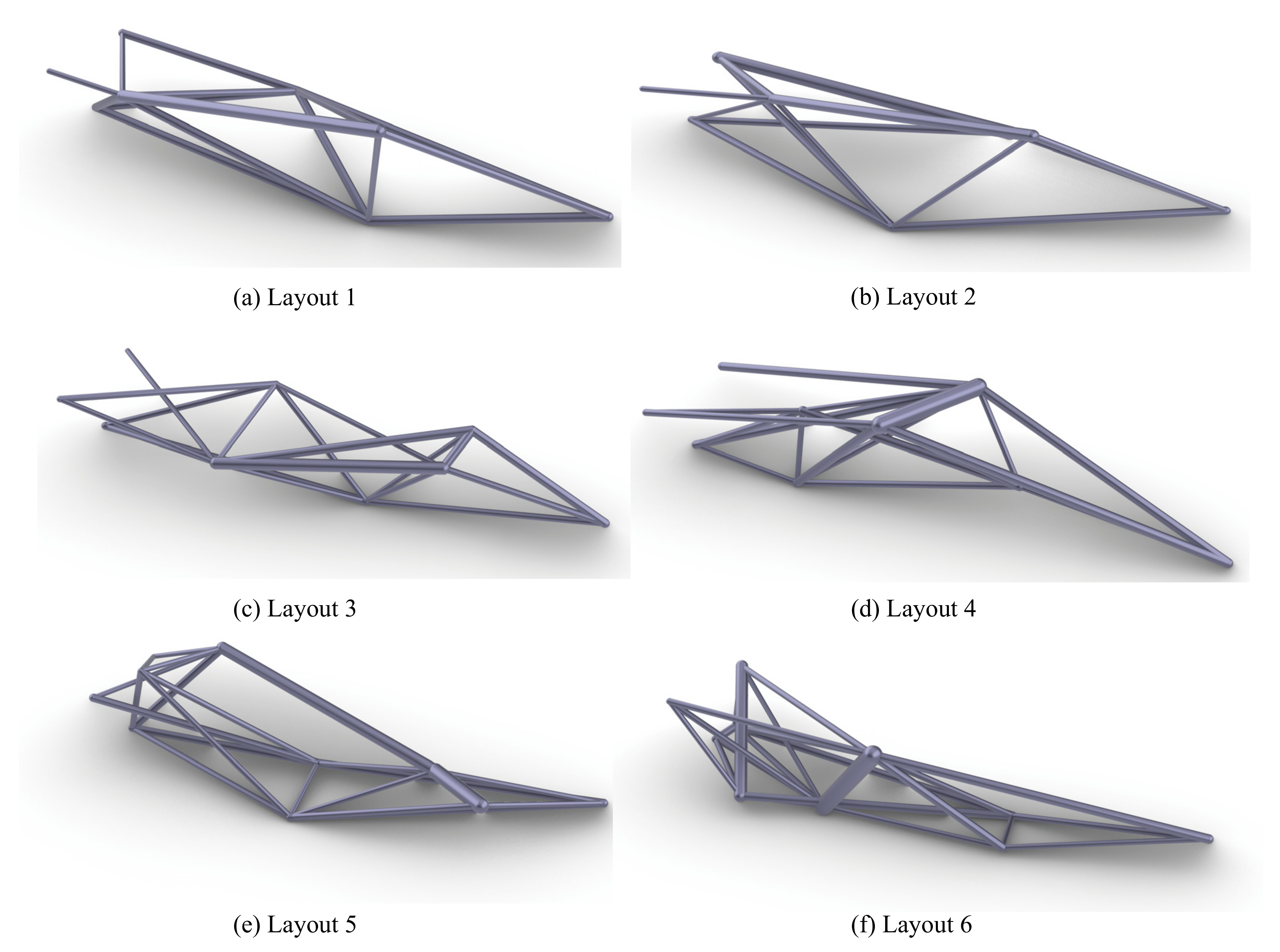
4.5. Three-Dimensional Cantilever Sundial Design

This design case is a test example of the KR-UCT algorithm on space trusses design, which is adapted from the sundial bracket truss built in Paternoster Square, London, UK [37]. A cantilever space truss with a length of 4634 mm is needed as the sundial bracket. Due to the need to read the scale based on the shadow of the sundial tip, the design of the sundial bracket is very strict with the stiffness of the space truss. The purpose of this experiment is to find the minimum truss weight under constraints in the three-dimensional design domain.

The design domain of this case is shown in Figure 14. This domain area only represents the essential node locations, and there is no mandatory geometric boundary on newly added nodes and bars. There are four fixed nodes in the design domain, among which nodes (1), (2), and (3) are pinned supported nodes, which are fixed on the wall in an isosceles triangle. Node (4) is the sundial tip, which is the loading node. It is fixed with a metal disk with holes of 300 mm in diameter and 6mm in thickness. The load is 50 N. The details of specified essential nodes and material property settings are summarized in

Table 17. Essential node coordinates in the three-dimensional cantilever sundial experiment.

Essential Node	Node Location (mm)	Node Label
$\left(1\right)$	$\left(0.0,0.0, 0.0\right)$	$\mathrm{Pinned} \mathrm{support}$
$\left(2\right)$	$\left(0.0,-0.483,0.595\right)$	$\mathrm{Pinned} \mathrm{support}$
$\left(3\right)$	$\left(0.0,0.483,0.595\right)$	$\mathrm{Pinned} \mathrm{support}$
$\left(4\right)$	$\left(4.634,0.772,-0.078\right)$	$\mathrm{Loading} \left(0, 0,-50 \mathrm{N}\right)$

and

Table 18. Material property settings in the three-dimensional cantilever sundial experiment.

Material Properties	Settings
$\mathrm{Young}’\mathrm{s} \mathrm{modulus}$	$193 \mathrm{GPa}$
$\mathrm{Density}$	$8000 \mathrm{kg}/{\mathrm{m}}^3$
$\mathrm{Yield} \mathrm{strength}$	$213 \mathrm{MPa}$

. The constraint combination for this experiment is $(g_1,g_2,g_3,g_4,g_6,g_7$). The parameters or formulas are expressed as follows: the allowable tension stress and the allowable compression stress ${\sigma }_c$ are both 0.6$f_y$; the allowable node displacement is limited to 2 mm; the allowable bar slenderness ratios are specified to be 220 for tension bars and 180 for compression bars; the minimum and maximum length of bars are 0.03 m and 5 m; in addition to the conventional constraint model, this example also requires that the angle between any two connecting bars should not exceed 1 degree; the cross-section of the bars used in this paper is the section of cold-formed thin-wall welded round steel tube (GB50018-2002). There are 61 groups of cross-section sizes from d25t1.5 to d245t4.0. In terms of structural load, this design case also considers the influence of the self-weight of the truss structure. The self-weight of the structure is evenly distributed on the end node of bars.

For the three different numbers of nodes varying from 8 to 10, the results generated by the KR-UCT algorithm for these three groups of experiments are illustrated in Figure 15. Two design results are presented for each group. Among the six generative design layouts, each layout has its own characteristics. In terms of weight, layout 3 is the lightest one, which receives the largest reward in the decision process. From the perspective of novelty, layout 4 may be an innovative design, which looks similar to a flapping wing.

In architectural structural design, structural weight and shape novelty is often weighed and considered according to the user or designer of the buildings, without a clear, quantifiable index. For example, in this experiment, KR-UCT can generate completely different layout schemes based on deterministic indicators through different decision trajectories. The final design scheme can be determined by comparing and selecting from various schemes. To facilitate a reference for comparison by subsequent studies, this paper lists the design results of layout 3 from multiple perspectives, as shown in Figure 16.

5. Conclusions

An MCTS-based reinforcement learning algorithm named KR-UCT is proposed to deal with continuous action spaces for truss layout design problems by using kernel regression. The algorithm solves the problem of sampling continuous action space when uniformly generating candidate action sets in a large-scale design space. It is a nonparametric regression way to sample the action space and generalize the information about action value between sampled actions and unexplored parts of the action space. As the number of iterations increases, the candidate action set is gradually expanded by appending actions with high confidence values from the design space. The value correlation between actions is mapped by the Gaussian function and Euclidean distance. In this sampling strategy, a modified upper confidence bound formula with kernel weight is proposed to evaluate the heuristics of sampled actions for both 2D and 3D cases. Several examples of generative design cases are carried out to demonstrate the effectiveness of the proposed algorithm. Excellent design performance is indicated by different experiments.

However, KR-UCT is limited in generating large-scale spatial structures such as grid structures or lattice shell structures since the three basic action sets require much more computing resources to generate complex structures. This limitation could be improved in the future from the following two aspects. The first is to develop new action sets. The layout elements of complex spatial truss structures can be disassembled into other basic structural elements (e.g., tetrahedrons and quadrangular pyramids). The difficulty of such research is how to deal with the complex and changeable spatial geometric relations and define the execution rules of relevant actions. The second is to improve the generalization ability of the model. A large amount of search data (decision experience) can be generated in advance for training deep neural networks to fit the expectation of reward value generated by different actions.

References

1. Shea, K.; Aish, R.; Gourtovai, M. Towards integrated performance-driven generative design tools. Autom. Constr. 2005, 14, 253–264. [Google Scholar] [CrossRef]
2. Amir, O.; Sigmund, O. Reinforcement layout design for concrete structures based on continuum damage and truss topology optimization. Struct. Multidiscip. Optim. 2013, 47, 157–174. [Google Scholar] [CrossRef]
3. Abdollahi, A.; Amini, A.; Hariri-Ardebili, M.A. An uncertainty-aware dynamic shape optimization framework: Gravity dam design. Reliab. Eng. Syst. Saf. 2022, 222, 108402. [Google Scholar] [CrossRef]
4. Watson, M.; Leary, M.; Brandt, M. Generative design of truss systems by the integration of topology and shape optimisation. Int. J. Adv. Manuf. Technol. 2022, 118, 1165–1182. [Google Scholar] [CrossRef]
5. Dorn, W. Automatic design of optimal structures. J. De Mec. 1964, 3, 25–52. [Google Scholar]
6. Zhu, S.; Ohsaki, M.; Hayashi, K.; Guo, X. Machine-specified ground structures for topology optimization of binary trusses using graph embedding policy network. Adv. Eng. Softw. 2021, 159, 103032. [Google Scholar] [CrossRef]
7. Tejani, G.G.; Savsani, V.J.; Patel, V.K.; Savsani, P.V. Size, shape, and topology optimization of planar and space trusses using mutation-based improved metaheuristics. J. Comput. Des. Eng. 2018, 5, 198–214. [Google Scholar] [CrossRef]
8. Gao, G.; Liu, Z.-y.; Li, Y.-b.; Qiao, Y.-f. A new method to generate the ground structure in truss topology optimization. Eng. Optim. 2017, 49, 235–251. [Google Scholar] [CrossRef]
9. Assimi, H.; Jamali, A.; Nariman-zadeh, N. Sizing and topology optimization of truss structures using genetic programming. Swarm Evol. Comput. 2017, 37, 90–103. [Google Scholar] [CrossRef]
10. Hagishita, T.; Ohsaki, M. Topology optimization of trusses by growing ground structure method. Struct. Multidiscip. O 2009, 37, 377–393. [Google Scholar] [CrossRef]
11. Stolpe, M. Truss optimization with discrete design variables: A critical review. Struct. Multidiscip. O 2016, 53, 349–374. [Google Scholar] [CrossRef]
12. Lieu, Q.X. A novel topology framework for simultaneous topology, size and shape optimization of trusses under static, free vibration and transient behavior. Eng. Comput. 2022. [Google Scholar] [CrossRef]
13. Shea, K.; Cagan, J. Languages and semantics of grammatical discrete structures. Artif. Intell. Eng. Des. Anal. Manuf. 1999, 13, 241–251. [Google Scholar] [CrossRef]
14. Kaveh, A.; Talatahari, S. Particle swarm optimizer, ant colony strategy and harmony search scheme hybridized for optimization of truss structures. Comput. Struct. 2009, 87, 267–283. [Google Scholar] [CrossRef]
15. Li, L.J.; Huang, Z.B.; Liu, F.; Wu, Q.H. A heuristic particle swarm optimizer for optimization of pin connected structures. Comput. Struct. 2007, 85, 340–349. [Google Scholar] [CrossRef]
16. Bellman, R. A Markovian decision process. J. Math. Mech. 1957, 6, 679–684. [Google Scholar] [CrossRef]
17. Raina, A.; McComb, C.; Cagan, J. Learning to design from humans: Imitating human designers through deep learning. J. Mech. Des. 2019, 141, 111102. [Google Scholar] [CrossRef]
18. Raina, A.; Cagan, J.; McComb, C. Design Strategy Network: A Deep Hierarchical Framework to Represent Generative Design Strategies in Complex Action Spaces. J. Mech. Des. 2021, 144, 4052566. [Google Scholar] [CrossRef]
19. Browne, C.B.; Powley, E.; Whitehouse, D.; Lucas, S.M.; Cowling, P.I.; Rohlfshagen, P.; Tavener, S.; Perez, D.; Samothrakis, S.; Colton, S. A survey of monte carlo tree search methods. IEEE Trans. Comput. Intell. AI Games 2012, 4, 1–43. [Google Scholar] [CrossRef]
20. Luo, R.; Wang, Y.; Xiao, W.; Zhao, X. AlphaTruss: Monte Carlo Tree Search for Optimal Truss Layout Design. Buildings 2022, 12, 641. [Google Scholar] [CrossRef]
21. Fenton, M.; McNally, C.; Byrne, J.; Hemberg, E.; McDermott, J.; O’Neill, M. Discrete planar truss optimization by node position variation using grammatical evolution. IEEE Trans. Evol. Comput. 2015, 20, 577–589. [Google Scholar] [CrossRef]
22. Miguel, L.F.F.; Lopez, R.H.; Miguel, L.F.F. Multimodal size, shape, and topology optimisation of truss structures using the Firefly algorithm. Adv. Eng. Softw. 2013, 56, 23–37. [Google Scholar] [CrossRef]
23. Pyrz, M. Discrete optimization of geometrically nonlinear truss structures under stability constraints. Struct. Optim. 1990, 2, 125–131. [Google Scholar] [CrossRef]
24. Sutton, R.S.; Barto, A.G. Reinforcement Learning: An Introduction, 2nd ed.; The MIT Press: Cambridge, MA, USA, 2018. [Google Scholar]
25. Maxwell, J.C.L. on the calculation of the equilibrium and stiffness of frames. Philos. Mag. J. Sci. 1864, 27, 294–299. [Google Scholar] [CrossRef]
26. Kocsis, L.; Szepesvári, C. Bandit Based Monte-Carlo Planning. In Proceedings of the European Conference on Machine Learning, Berlin, Germany, 18–22 September 2006; pp. 282–293. [Google Scholar]
27. Chaslot, G.M.J.; Winands, M.H.; Herik, H.J.V.D.; Uiterwijk, J.W.; Bouzy, B. Progressive strategies for Monte-Carlo tree search. New Math. Nat. Comput. 2008, 4, 343–357. [Google Scholar] [CrossRef]
28. Yee, T.; Lisý, V.; Bowling, M.H.; Kambhampati, S. Monte Carlo Tree Search in Continuous Action Spaces with Execution Uncertainty. In Proceedings of the IJCAI, New York, NY, USA, 9–16 July 2016; pp. 690–697. [Google Scholar]
29. Razani, R. Behavior of fully stressed design of structures and its relationshipto minimum-weight design. AIAA J. 1965, 3, 2262–2268. [Google Scholar] [CrossRef]
30. Deb, K.; Gulati, S. Design of truss-structures for minimum weight using genetic algorithms. Finite Elem. Anal. Des. 2001, 37, 447–465. [Google Scholar] [CrossRef]
31. Luh, G.-C.; Lin, C.-Y. Optimal design of truss structures using ant algorithm. Struct. Multidiscip. Optim. 2008, 36, 365–379. [Google Scholar] [CrossRef]
32. Wu, C.-Y.; Tseng, K.-Y. Truss structure optimization using adaptive multi-population differential evolution. Struct. Multidiscip. Optim. 2010, 42, 575–590. [Google Scholar] [CrossRef]
33. Construction, A. Manual of Steel Construction: Allowable Stress Design; AISC: Chicago, IL, USA, 1989. [Google Scholar]
34. Yang, Y.; Soh, C.K. Automated optimum design of structures using genetic programming. Comput. Struct. 2002, 80, 1537–1546. [Google Scholar] [CrossRef]
35. Shrestha, S.M.; Ghaboussi, J. Evolution of optimum structural shapes using genetic algorithm. J. Struct. Eng. 1998, 124, 1331–1338. [Google Scholar] [CrossRef]
36. Gutiérrez, N. Optimización Estructural de Armaduras Utilizando Algoritmos Genéticos. Master’s Thesis, Universidad Autónoma de Querétaro, México City, Mexico, 2007. [Google Scholar]
37. Shea, K.; Zhao, X. A novel noon mark cantilever support: From design generation to realization. In Proceedings of the IASS 2004: Shell and Spatial Structures from Models to Realization, Montpellier, France, 20–24 September 2004. [Google Scholar]
Figure 1. Truss layout MDP model represented by the search tree.
Applsci 12 08227 g001
Figure 2. Design domain of the 17-bar planar truss.
Applsci 12 08227 g002
Figure 3. Optimal truss layout generated in the 17-bar experiment.
Applsci 12 08227 g003
Figure 4. Action-taking process for constructing an optimal truss in the 17-bar experiment.
Applsci 12 08227 g004
Figure 5. Uniform distribution of node candidate set in the UCT algorithm.
Applsci 12 08227 g005
Figure 6. Heuristic distribution of node candidate sets in the KR-UCT algorithm.
Applsci 12 08227 g006
Figure 7. Design domain of 10-bar planar truss.
Applsci 12 08227 g007
Figure 8. Generated layouts for the 10-bar planar truss experiment. (a) maxp = 6, weight = 2153.87 kg; (b) maxp = 7, weight = 1968.72 kg; (c) maxp = 8, weight = 1852.46 kg; (d) maxp = 9, weight = 2122.05 kg.
Applsci 12 08227 g008
Figure 9. Multiple competitive truss layouts generated by the KR-UCT algorithm.
Applsci 12 08227 g009
Figure 10. Design domain of the 39-bar planar truss.
Applsci 12 08227 g010
Figure 11. Optimal truss layout generated for the 39-bar experiment.
Applsci 12 08227 g011
Figure 12. Design domain of the long-span bridge truss.
Applsci 12 08227 g012
Figure 13. Optimal truss layout generated for long-span bridge truss experiment.
Applsci 12 08227 g013
Figure 14. Design domain of the three-dimensional cantilever sundial truss.
Applsci 12 08227 g014
Figure 15. Generated layouts in the three-dimensional cantilever sundial experiment. (a) maxp = 8, weight = 38.7 kg; (b) maxp = 8, weight = 46.5 kg; (c) maxp = 9, weight = 37.2 kg; (d) maxp = 9, weight = 41.6 kg; (e) maxp = 10, weight = 44.3 kg; (f) maxp = 10, weight = 46.7 kg.
Applsci 12 08227 g015
Figure 16. Multi-view presentation of layout 3. (a) Top view; (b) perspective view; (c) front view; (d) right view.
Applsci 12 08227 g016