Two-Dimensional Profile Simulation Model for Five-Axis CNC Machining with Bull-Nose Cutter

Abstract

Surface topography is closely related to fatigue strength and mating accuracy of workpieces. The profile method is widely adopted to evaluate surface topography. In the present study, a 2D profile simulation model of five-axis CNC machining with a bull-nose cutter is proposed to predict the surface topography of a machined workpiece. To this end, a simplified scallop model is established by analyzing the geometry and motion of the bull-nose cutter. Then, the principles of the 2D profile simulation model for plane and free-form surfaces are described to provide the basis for building 2D profile simulation models. After that, 2D profiles are obtained directly from CL data, tool parameters, and workpiece design models, and an algorithm is proposed to obtain 2D profiles. Finally, the proposed algorithm is verified by different machining experiments on plane and free-form surfaces. The results show that the simulation and measurement results are in good agreement. The proposed simulation model for five-axis CNC machining with a bull-nose cutter can be effectively applied to simulate 2D profiles of plane and free-form surfaces. The present study is expected to provide a reference for optimizing process parameters.

1. Introduction

Milling is an important machining process widely used in manufacturing free-form surfaces. Bull-nose cutters have superior characteristics, such as curvature adaptiveness, so they are increasingly used in CNC machining. Applying bull-nose cutters for machining complex convex surfaces can reduce machining time and improve machining quality compared to ball-end cutters [1]. Surface topography is defined as the surface geometry of the machined workpiece after cutting, which includes the surface profile and surface quality [2] and is closely related to the fatigue strength and mating accuracy of the workpiece. The better the surface topography, the higher the workpiece’s fatigue performance, corrosion resistance, stability, and reliability [3]. Further investigations have revealed that surface topography is affected by tool type, tool path [3,4,5,6], machining parameters [4,7,8,9], and tool orientation [3,8,10,11,12,13].

Because surface topography has a large impact on the performance of a workpiece, a large number of scholars have conducted research on surface topography prediction methods. Currently, surface topography prediction methods can be mainly categorized into experimental methods and analytical models. In this regard, extensive cutting experiments have been carried out, and empirical models have been established through data analysis. Michal Gdula et al. [14] conducted cutting experiments on five-axis milling with bull-nose cutters, analyzed the effect of tool orientation and workpiece radius of the curvature on surface roughness and topography, and developed an empirical model. Khorasani et al. [15] developed a neural milling process model based on experimental data to predict surface roughness during milling. Hasan et al. [16] analyzed experimental data and developed a surface roughness prediction model using neural networks and genetic algorithms. Cao et al. [17] proposed a GAN algorithm to predict surface roughness. Moayyedian et al. [18] investigated the effects of different cutting parameters on surface roughness by experiments and proposed a mathematical model to predict the signal-to-noise (S/N) ratio. Dayan et al. [19] developed a mathematical relationship between the surface roughness, cutting speed, feed rate, and cutting depth based on experimental data. Kumar et al. [20] carried out experiments and studied the variation of surface roughness of Inconel 718 under different machining conditions and developed second-order surface roughness models to predict the surface roughness of a workpiece. It should be indicated that although these proposed models obtained by cutting experiments for topography or roughness of the surface are accurate, they are only suitable for the materials studied. Furthermore, the formation process of milling surface topography cannot be theoretically analyzed.

Reviewing the literature also indicates that numerous analytical models have been proposed for surface topography. Layegh et al. [21] established a trajectory model for the cutting edge of a ball-end cutter, then calculated the intersection between the trajectory and the cutting plane in the vertical feed direction, and finally established a surface topography analysis and prediction model for five-axis CNC milling. Yuan et al. [22] established a surface roughness prediction model to study the flat-end cutter milling process, considering the runout and minimum chip thickness in the calculations. Gao et al. [23] established a motion trajectory equation of the cutting edge to obtain a surface topography prediction model of flat-end and ball-end cutters. Zhang et al. [24] proposed an iterative method to simulate the surface topography of milling with a ball-end cutter. Cai et al. [25] analyzed the motion of the cutting edge of a ball-end cutter and established a surface topography model based on the Z-Map model. Peng et al. [26] established a cutting-edge trajectory model to simulate the surface topography of a micro-ball-end cutter. In this regard, numerous parameters, including tool orientation, tremor, runout, cutting force, and plastic deformation, were considered in the calculation. Further, this method is also based on the Z-Map. Wei et al. [27] analyzed the motion of the cutting edge of a ball-end cutter and constructed a 3D surface topography model accordingly. Based on the N-buffer method and combined with inverse kinematic transformation of five-axis machining, Quinsat et al. [28] proposed a 3D surface topography model for machining. Wang et al. [29] combined geometric and mechanical models and established a surface roughness prediction model considering the influence of elastic and plastic deformation. Based on the Z-Map, Zhou et al. [30] established a model to predict the surface topography of four-axis milling by analyzing the cutting-edge motion of a bull-nose cutter. However, this method does not consider tool deformation, tool wear, or vibration in machining. Lavernhe et al. [31] used the N-Buffer method to develop a 3D topography prediction model for free-form surfaces machined by a bull-nose cutter, and investigated the effect of inclination angle on surface topography using the prediction model and milling experiments. Recently, Bizzarri et al. [32] proposed a symbolic–numerical approach for approximating the curve. This approach is an efficient method for approximating the curve using graphs of critical points.

Bull-nose cutters are increasingly used in CNC machining due to their curvature adaptiveness. However, most current studies focus on modeling surface topography for machining with ball-end and flat-end cutters, while only a few focus on using bull-nose cutters. Simultaneously, the prediction model of surface topography after machining by a five-axis CNC with a bull-nose cutter can be used to verify the machining parameters and provide a theoretical basis to optimize them. Additionally, the profile method is a widely adopted method to evaluate surface topography. Therefore, a 2D profile simulation model is proposed in this study to predict the surface topography of five-axis CNC machining with a bull-nose cutter. This model and the corresponding simulation algorithm are presented in Section 2 and Section 3, respectively. Simulation and machining experiments for the bull-nose cutter machining plane and free-form surface are discussed in Section 4. Finally, the main achievements and conclusions are summarized in Section 5.

2. Model of Surface Topography with a Bull-Nose Cutter

During the machining process, the cutter makes translational and rotational movements, which are controlled by the machine tool. When the cutter contacts the workpiece, material removal occurs, leaving traces on the workpiece’s surface and forming the surface topography. Figure 1 shows the model of the bull-nose cutter, in which $R$ and $r$ are the cutter’s radius and the corner radius, respectively. Moreover, $L$ and $LN$ denote the cutter length and the length of the cutting edge, respectively. The cutting edge can be divided into three parts: the bottom surface $A1$, the circular surface $A2$, and the cylindrical surface $A3$.

Geometrically, the surface topography of the workpiece is a function of the step distance $d$ between adjacent cutting contact trajectories and the amount of feed per tooth $f_z$. During machining, the parameter $f_z$ is small, so the scallops left by cutter movement can be considered part of the annulus. Figure 2 shows that the surface topography of the workpiece varies with tool orientation. During the finishing process, the material is removed by the circular surface $A2$ of the cutter due to the small depth of the cut. Figure 2 also reveals that the surface topography of the machined workpiece consists of scallops. Scallops are formed by the movement of the cutting edge of the bull-nose cutter. Without considering the phase angle, each scallop is adjacent to at least four scallops and usually adjacent to six scallops. Thus, it is necessary to describe these surface scallops to describe the surface topography of the workpiece.

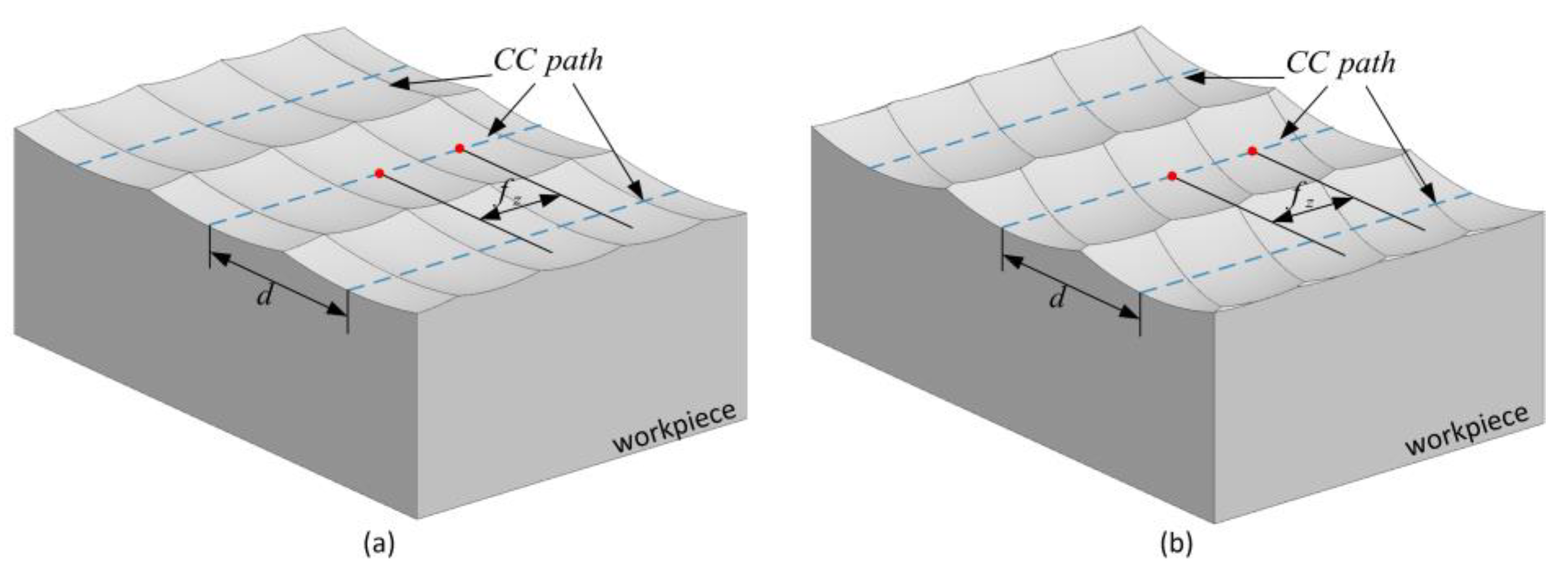
2.1. Calculation of Scallops

Each scallop can be considered an envelope of moving annulus. The parametric equation of an annulus in the tool coordinate system $C{S}_T$ can be expressed in the form below:

$$\mathrm{C}\left(\alpha ,\beta \right)=\left[\begin{array}{c}x\left(\alpha ,\beta \right)\\ y\left(\alpha ,\beta \right)\\ z\left(\alpha ,\beta \right)\end{array}\right]=\left[\begin{array}{c}\left[\left(R-r\right)+r\cdot \sin \alpha \right]\cdot \cos \beta \\ \left[\left(R-r\right)+r\cdot \sin \alpha \right]\cdot \sin \beta \\ r\cdot \left(1-\cos \alpha \right)\end{array}\right].$$

(1)

In five-axis CNC machining, the transformation matrix of the tool coordinate system $C{S}_T$ to the workpiece coordinate system $C{S}_W$ is:

$$M_{T-W}=\left[\begin{array}{cccc}{X}_{T-W}& Y_{T-W}& Z_{T-W}& O_{T-W}\\ 0& 0& 0& 1\end{array}\right],$$

(2)

where $X_{T-W}$, $Y_{T-W}$, and $Z_{T-W}$ represent the axes of the tool coordinate system $C{S}_T$ in the workpiece coordinate system $C{S}_W$, and $O_{T-W}$ represents the cutter location (CL) in the workpiece coordinate system $C{S}_W$. In the workpiece coordinate system $C{S}_W$, the parametric equation of the annulus is:

$$\left[\begin{array}{c}{x}_W\left(\alpha ,\beta \right)\\ y_W\left(\alpha ,\beta \right)\\ z_W\left(\alpha ,\beta \right)\\ 1\end{array}\right]=M_{T-W}\cdot \left[\begin{array}{c}x\left(\alpha ,\beta \right)\\ y\left(\alpha ,\beta \right)\\ z\left(\alpha ,\beta \right)\\ 1\end{array}\right].$$

(3)

The cutter and the workpiece are tangent at the CC point, so the scallop is tangent to the surface of the workpiece. For an arbitrary scallop, the approximate surface of the scallop at the CC point in the local coordinate system $\left\{CC,T_{\max }^C,T_{\min }^C,N\right\}$ can be expressed in the form below:

$$z=\frac{1}{2}\left({\kappa }_1{x}^2+{\kappa }_2{y}^2\right)+o\left(x^2+y^2\right),$$

(4)

where ${\kappa }_1$ and ${\kappa }_2$ are the principal curvatures of the bull-nose cutter at the CC point. This equation is the second-order approximation of the annulus surface at the CC point, and it is actually the equation of the so-called oscullating paraboloid [33]. This equation describes the geometric properties of the bull-nose cutter at the CC point. It is used in tool motion planning, tool orientation optimization, and other problems in CNC machining.

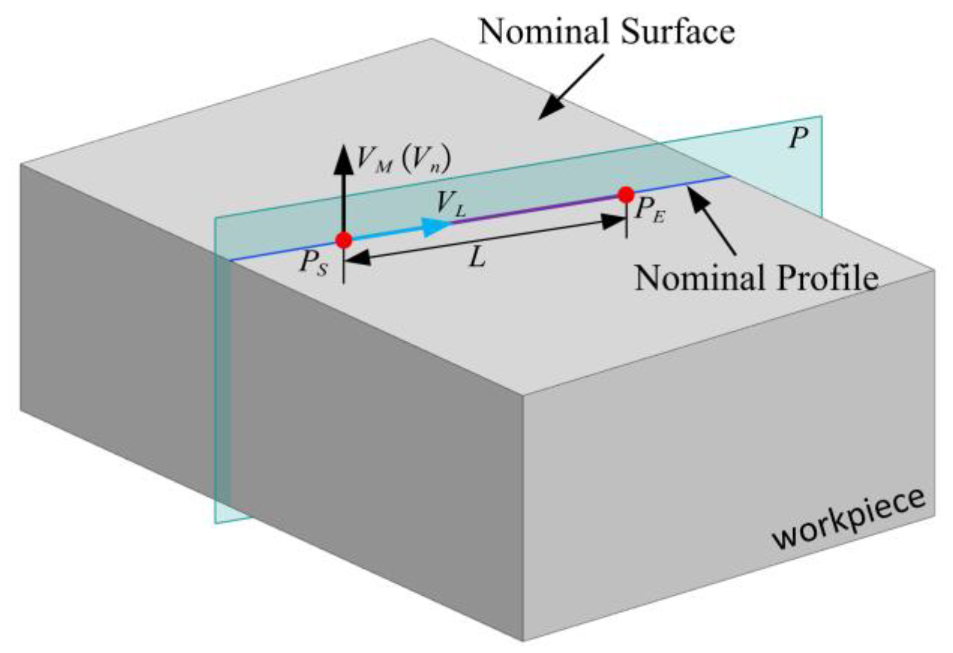
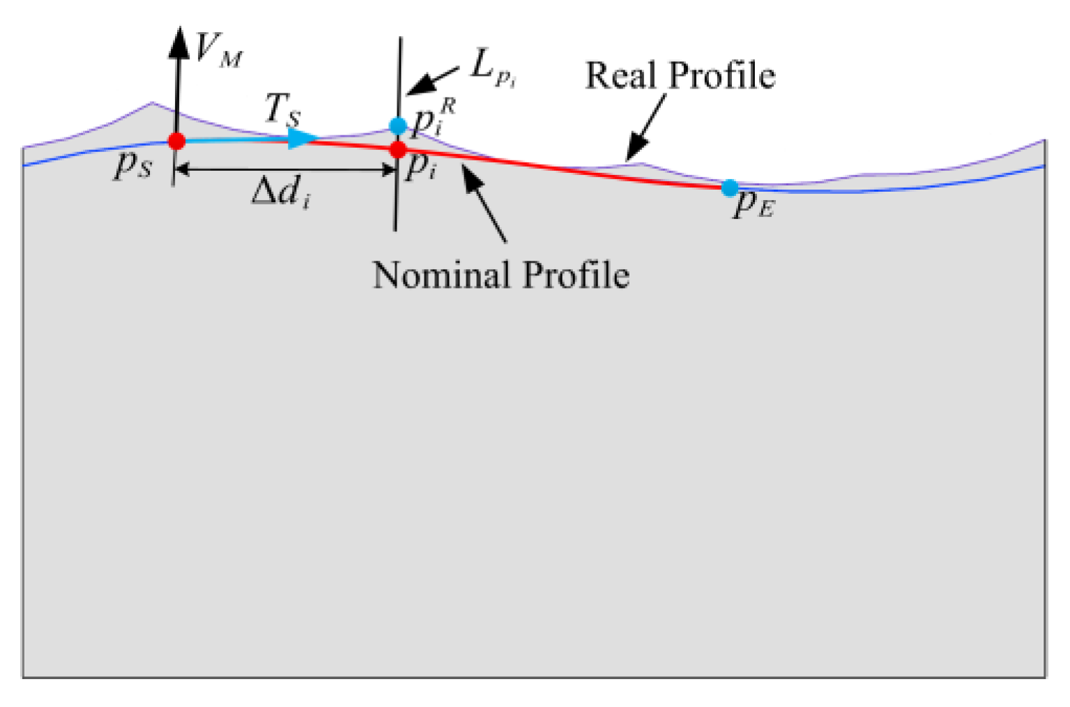
2.2. The Principle of 2D Profile Measurement

The profile method is major for evaluating surface topography, and it is widely used in machining. A 2D profile is obtained by intersecting a specified plane $P$ with the surface. The plane $P$ is determined by the 2D profile measurement line $V_L$, which is a straight line that connects the start point $P_S$ and end point $P_E$, and the normal vector $V_n$ of the nominal surface at the start point $P_S$. Usually, $V_n$ and $V_L$ are not parallel or perpendicular. The normal vector $n_P$ of the plane $P$ is a unit vector. Thus, $n_P$ can be expressed in the form below:

$$n_P=\frac{V_L\times V_n}{\left|V_L\times V_n\right|}.$$

(5)

The length $L$ between $P_S$ and $P_E$ is determined according to the standard. The measuring direction $V_M$ is on plane $P$ and perpendicular to $V_L$, and it is a unit vector to which the probe is parallel during measurement. Thus, $V_M$ can be expressed in the form below:

$$V_M=n_P\times V_L.$$

(6)

Then, the points and vectors of 2D profile measurement are described separately for planes and free-form surfaces.

For a plane surface, the start and end points are on the nominal surface. Thus, the 2D profile measurement line $V_L$ is on the nominal surface, and it is also perpendicular to the normal vector $V_n$ of the nominal surface at the start point $P_S$. Therefore, the measuring direction $V_M$ is parallel to the ... These points and vectors are shown in Figure 3.

However, for a free-form surface, these points and vectors are different from those on a plane. First of all, points $P_1$ and $P_2$ are taken on the nominal surface to determine the 2D profile measurement line $V_L$. The 2D profile measurement line $V_L$ satisfies:

$$V_L=\frac{P_2-P_1}{\left|P_2-P_1\right|}.$$

(7)

Then, $P_1$ is used as the start point of the 2D profile measurement line $V_L$, and is denoted $P_S$. The point along the 2D profile measurement line $V_L$ with distance $L$ from the start point $P_S$ is the end point $P_E$. Normally, $V_L$ is not perpendicular to the normal vector $V_n$ of the nominal surface at $P_S$. These points and vectors are presented in Figure 4. It is worth noting that point $P_E$ is not on the nominal surface if the surface is a free-form surface, as shown in Figure 4 and Figure 5.

The process of obtaining a nominal profile can be summarized as follows: the stylus parallel to the measuring direction $V_M$ starts from starting point $P_S$, follows the measuring line direction $V_L$, obtains a surface profile of a certain length $L$, and ends at the endpoint $P_E$. The above describes the points and vectors of 2D profile measurement, which is the foundation of the simulation algorithm of the 2D profile.

3. Simulation Algorithm of the 2D Profile

3.1. Calculation of the Nominal Profile

Nominal profile refers to the profile of intersection between the nominal surface and plane $P$. The nominal profile of a plane surface is a line segment of length $L$ that passes the starting point $P_S$ along the 2D profile measurement line $V_L$. Thus, the point $p_i$ on the nominal profile of a plane surface can be mathematically expressed in the form below:

$$p_i=P_S+l\prime \cdot V_L,$$

(8)

where $0\le l\prime \le L$.

However, the nominal profile of a free-form surface is different from that of a plane. Assume that, in the workpiece coordinate system, the parametric equation of the nominal surface can be expressed as follow:

$$r=r\left(u,v\right),$$

(9)

where $u$ and $v$ are parameters of nominal surface. Figure 6 shows that the nominal profile of the free-form surface is a plane curve that passes the start point $P_S$. The start and end points of this curve are $p_S$ and $p_E$, respectively. Obviously, the point $p_S\left(u_S,v_S\right)$ is on the nominal surface. Line $L_{P_E}$ passes through point $P_E$, and it is parallel to $V_M$. It is worth noting that $p_E$ is the intersection of line $L_{P_E}$ with the nominal surface.

As shown in Figure 7, the vector $T_S$ is on plane $P$, which is the tangent vector of the nominal profile at $p_S$. $T_S$ can be expressed in the form below:

$$T_S=\frac{V_n\times n_P}{\left|V_n\times n_P\right|}.$$

(10)

$T_S$ can also be written in the following form:

$$T_S=r_u\cdot \delta u_{T_S}+r_v\cdot \delta v_{T_S},$$

(11)

where $r_u$ and $r_v$ are the tangent vectors along with the parameters $u$ and $v$, respectively, at $p_S$. The ratio of $\delta v_{T_S}$ to $\delta u_{T_S}$ (which is hereafter called $k$) can be used to describe the direction $T_S$. The angle between the principal direction $T_{\max }$ and $T_S$ is $\omega$, so the following equation holds:

$$T_{\max }\cdot T_S=\left|T_{\max }\right|\cdot \left|T_S\right|\cdot \cos \omega ,$$

(12)

where

$$T_{\max }=r_u\cdot \delta u_{\max }+r_v\cdot \delta v_{\max }.$$

(13)

The ratio of $\delta v_{\max }$ to $\delta u_{\max }$ can also be used to describe the direction $T_{\max }$. Combining Equations (10)–(13) yields the following expression:

$$k=\frac{-\left(\frac{2\cdot B\cdot C}{A^2\cdot {\cos }^2\omega }-2r_u\cdot r_v\right)\pm \sqrt{{\left(\frac{2\cdot B\cdot C}{A^2\cdot {\cos }^2\omega }-2r_u\cdot r_v\right)}^2-4\left(\frac{C^2}{A^2\cdot {\cos }^2\omega }-r_v{}^2\right)\left(\frac{B^2}{A^2\cdot {\cos }^2\omega }-r_u{}^2\right)}}{2\cdot \left(\frac{C^2}{A^2\cdot {\cos }^2\omega }-r_v{}^2\right)},$$

(14)

where $A=\sqrt{\delta u_{\max }{}^2\cdot r_u{}^2+2\delta u_{\max }\cdot \delta v_{\max }+\delta v_{\max }{}^2\cdot r_v{}^2}$, $B=\delta u_{\max }\cdot r_u{}^2+\delta v_{\max }\cdot r_u\cdot r_v$, and $C=\delta u_{\max }\cdot r_u\cdot r_v+\delta v_{\max }\cdot r_v{}^2$.

Any point $p_i$ on the nominal profile can be expressed as follows:

$$p_i=r\left(u_s+\Delta u_i,v_s+\Delta v_i\right),$$

(15)

where $\Delta u_i$ and $\Delta v_i$ are the differences of the parameters between $p_i$ and $p_S$. Figure 8 shows that within the nominal profile, the interval between any point $p_i$ and the starting point $p_S$ of the nominal contour is $\Delta d_i$. When $\Delta d_i$ is infinitely small, the point $p_i$ can be considered to be on the tangent vector $T_S$, so it satisfies the following equation:

$$\overrightarrow{p_i-p_E}=\frac{T_S}{\left|T_S\right|}\cdot \Delta d_i,$$

(16)

where

$$\overrightarrow{p_i-p_E}=r_u\cdot \Delta u_i+r_v\cdot \Delta v_i.$$

Further, because $\Delta v_i=k\cdot \Delta u_i$, we can obtain:

$$\{\begin{array}{l}\Delta u_i=\frac{\Delta d_i}{\sqrt{r_u{}^2+2k\cdot r_u\cdot r_v+k^2\cdot r_v{}^2}}\\ \Delta v_i=k\cdot \Delta u_i\end{array}.$$

(17)

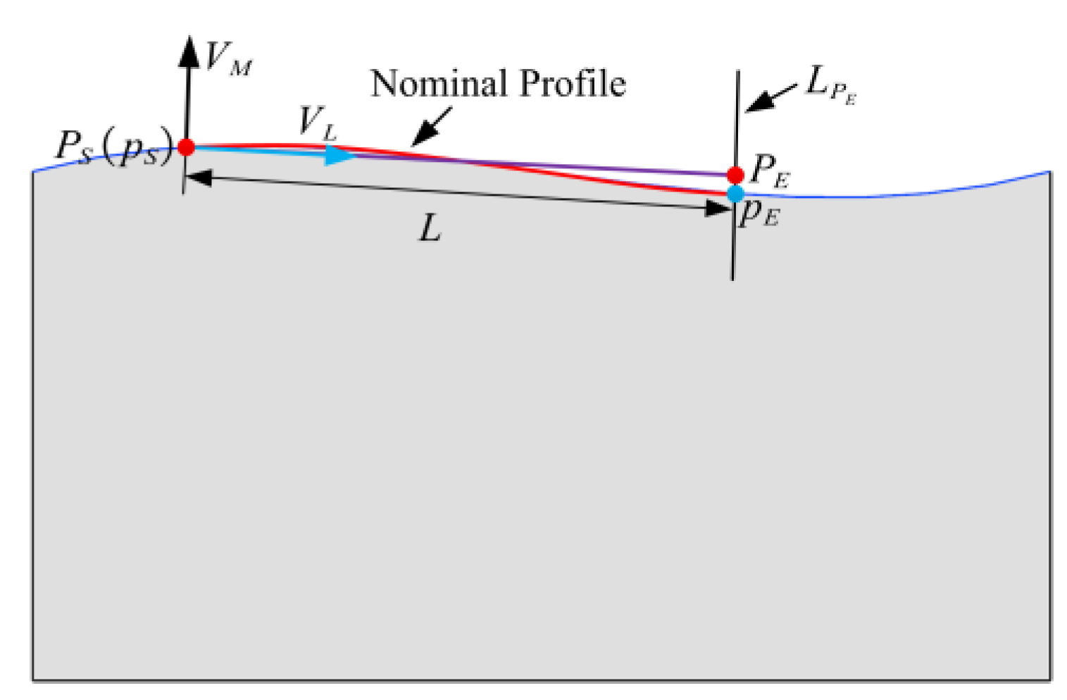
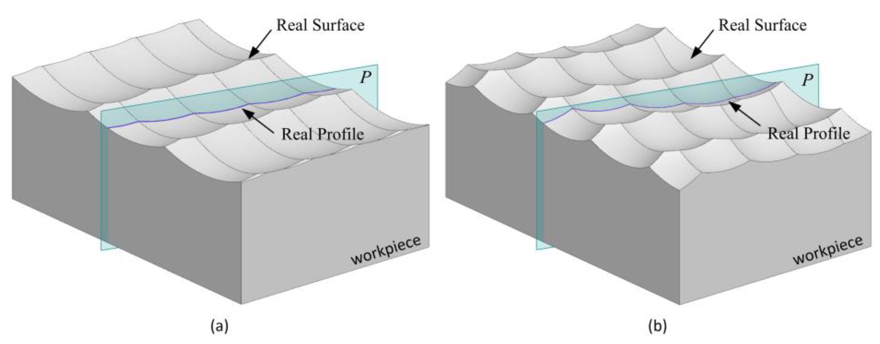
3.2. Calculation of the Real Profile

The real profile refers to the line of intersection between the real surface and the plane $P$, which is presented in Figure 9. We found that the simulation model can be considered a series of scallops, each defined by the CC point, the principal direction, and the principal curvature.

In a free-form surface as an example, line $L_{p_i}$ passes through point $p_i$, and it is parallel to the measuring direction $V_M$. Figure 10 shows that the intersection of line $L_{p_i}$ and the real profile is point $p_i^R$, which corresponds to the nominal point $p_i$.

Line $L_{p_i}$ intersects some scallops, and the distance between the intersection point $p_i^m$ and the point $p_i$ is denoted $l_i^m$, where m is the index of the CC point corresponding to the scallop, as shown in Figure 11. The point corresponding to the minimum distance value $l_{i,\min }$ is the intersection point $p_i^R$ of $L_{p_i}$ with the real profile.

The flowchart for calculating the 2D profile is shown in Figure 12. The 2D profile can be obtained through the following steps:

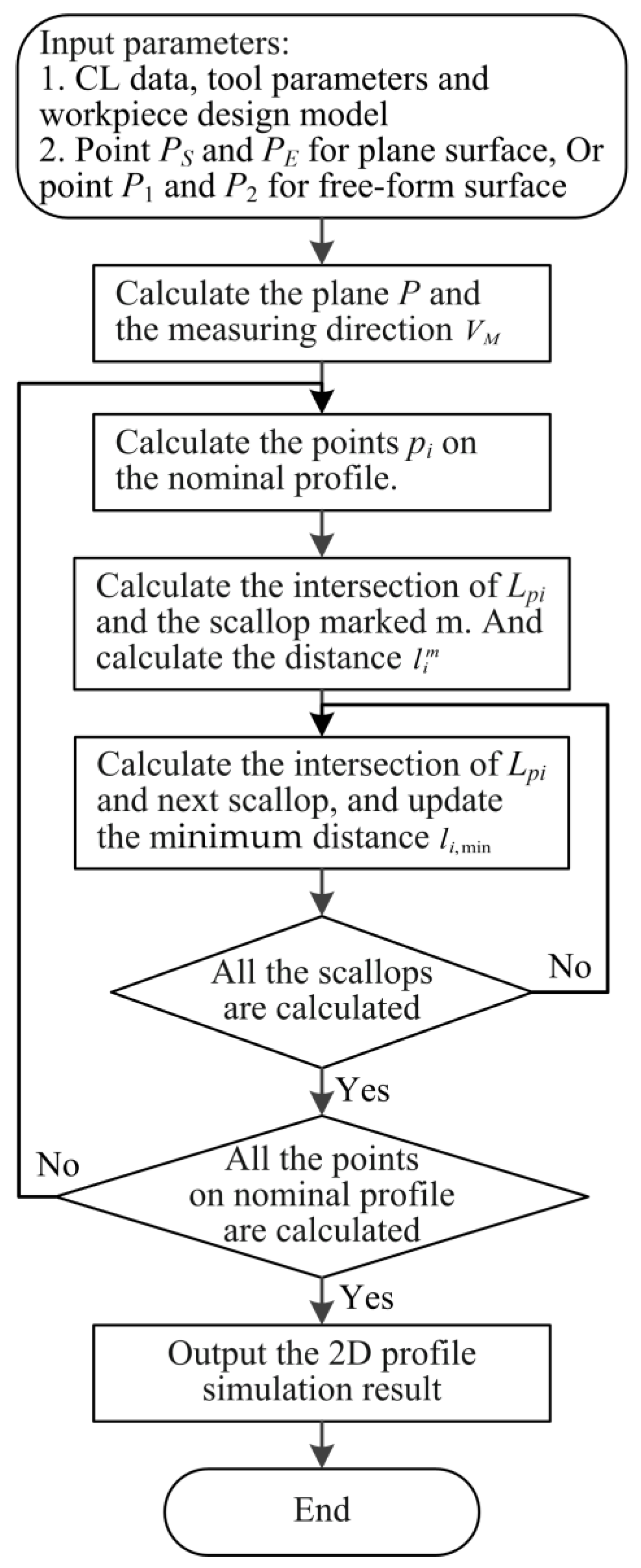
• Input the CL data, tool parameters, and the workpiece design model. Input points $P_S$ and $P_E$ for a plane surface, or input points $P_1$ and $P_2$ for a free-form surface.
• Calculate plane $P$ according to the 2D profile measuring line $V_L$ and the normal vector $V_n$ of the nominal surface at the start point $P_S$. Then calculate the measuring direction $V_M$ by using Equation (6).
• Calculate the points $p_i$ on the nominal profile.
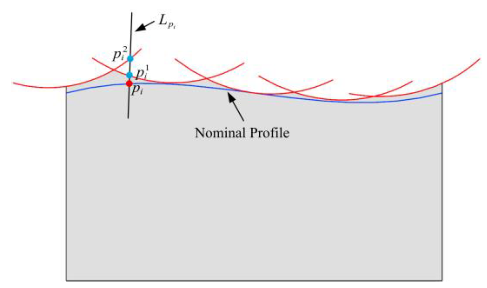
• Calculate the intersection of $L_{p_i}$ and the scallop marked m according to the point $p_i$ and the measurement direction $V_M$. Then calculate the distance $l_i^m$.
• Calculate the intersection of $L_{p_i}$ and the next scallop, and update the minimum distance $l_{i,\min }$.
• Repeat Step (5) for each scallop to obtain the minimum distance $l_{i,\min }$ and the real profile’s intersection point $p_i^R$.
• Repeat Steps (3) to (6) for each point $p_i$ to get the real profile.
• The main objective of 2D profile simulation is to find the difference between the real profile and the nominal profile. Hence, the simulation algorithm of the 2D profile can be obtained.

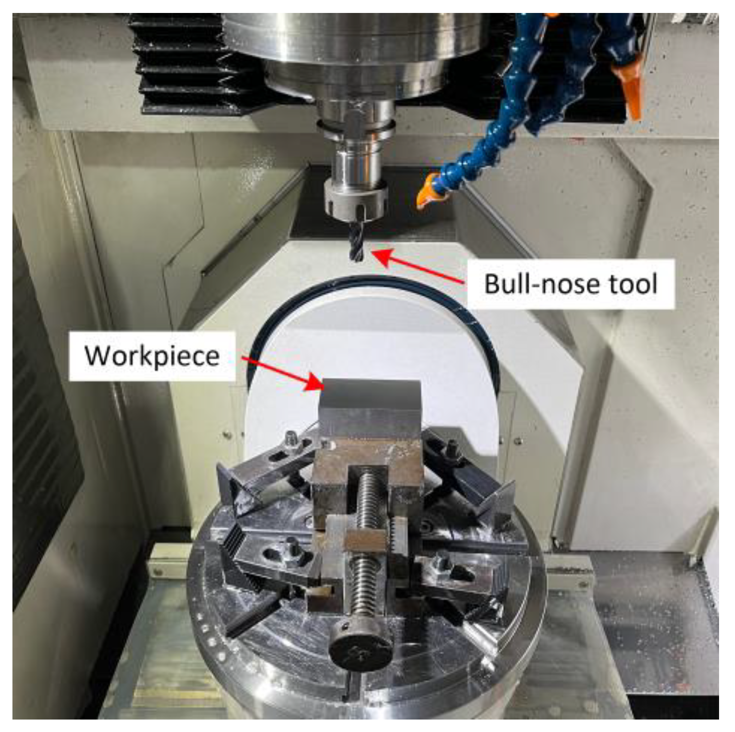
4. Simulation and Experiments

To verify the accuracy of the 2D profile simulation model, cutting experiments were carried out using a JD GR200T five-axis CNC machine. The material to be machined was 2Cr13 steel. Larger cutting parameters were used in the finishing process for easy observation and comparison. There are two main machining experiments: plane and free-form surface machining.

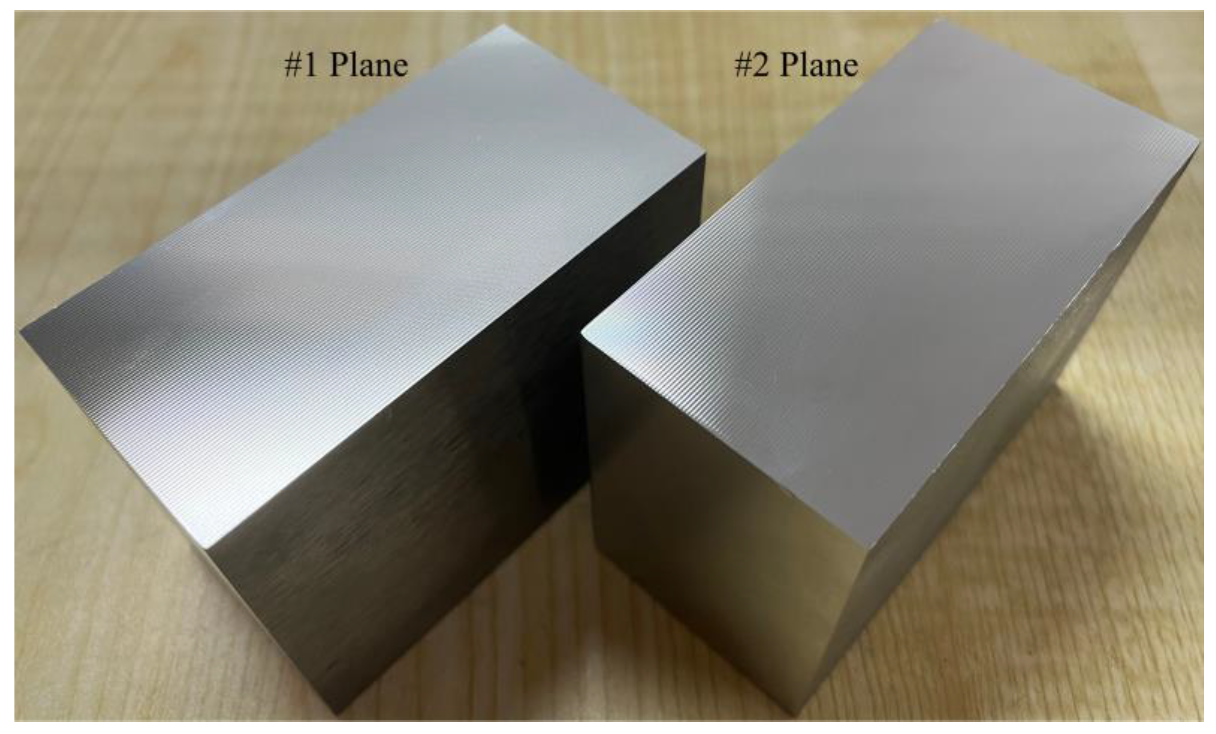
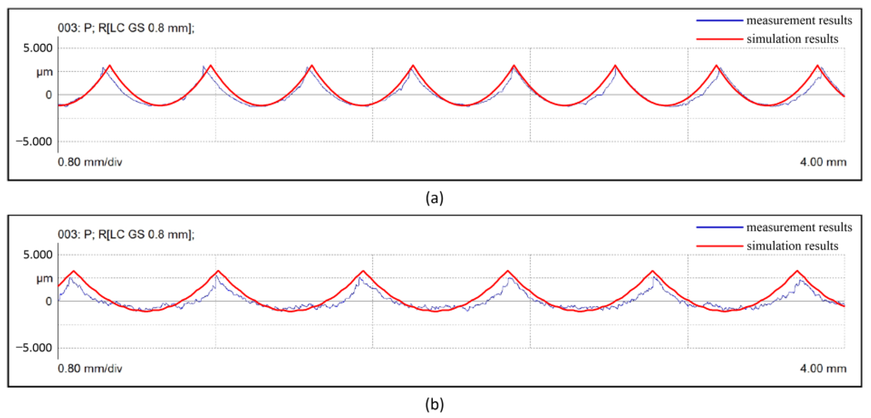
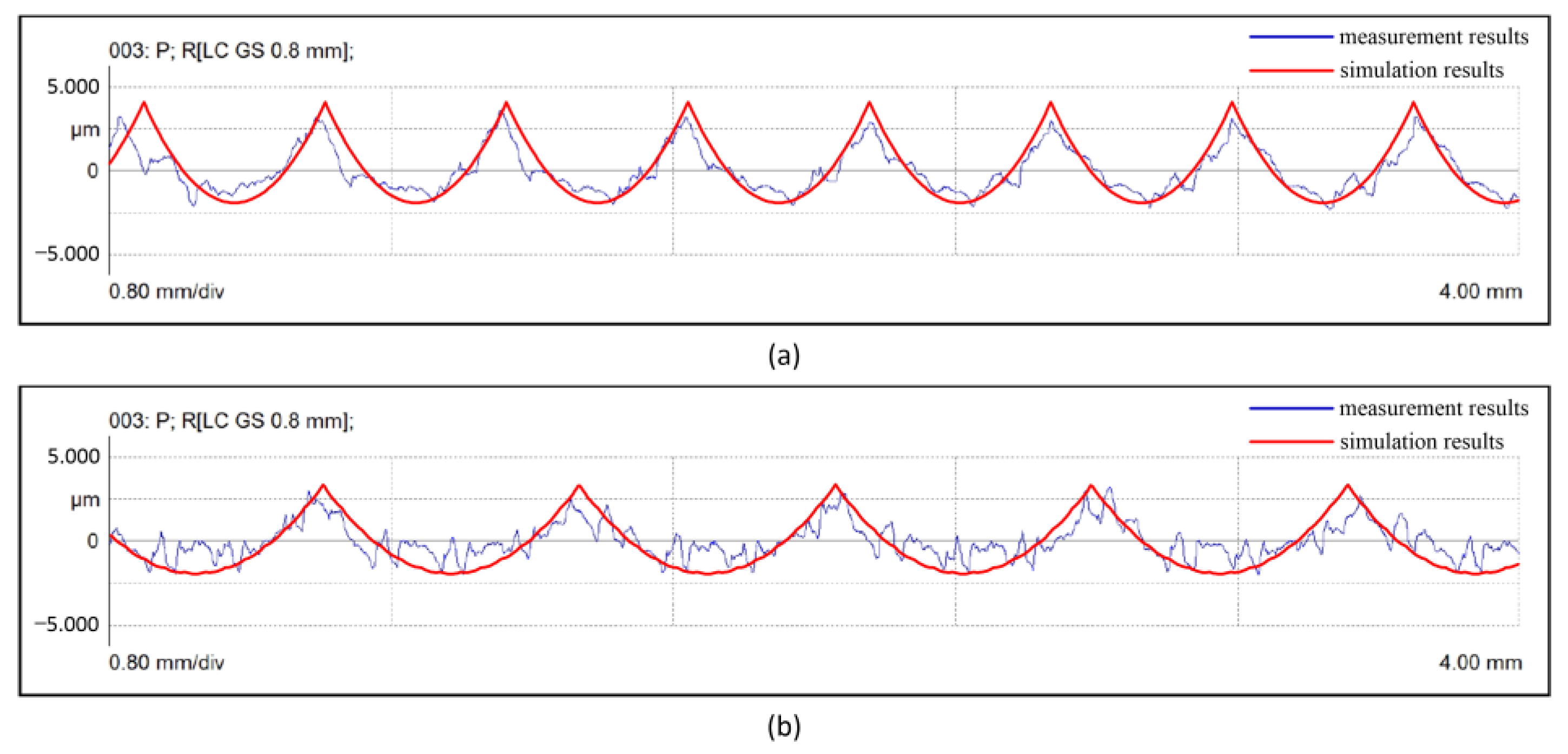
4.1. Milling Plane Surface with Bull-Nose Cutter

The tool used in the machining experiment was a four-tooth bull-nose cutter with a radius of $R=5\mathrm{mm}$ and a corner radius of $r=3\mathrm{mm}$. Figure 13 shows the configuration of the machining experiment. The experiment blank was 82 mm long, 42 mm wide, and 62 mm high.

Table 1. Cutting parameters used in the plane-surface machining experiment.

Spindle speed	4000 rpm
Cutting depth	0.2 mm
Stepover	0.5 mm
Feed rate per tooth	0.05 mm/tooth

shows the cutting parameters for the machining experiments.

Table 2. Tool orientation for the plane-surface machining experiment.

	Inclination Angle (°)	Tilt Angle (°)
Plane #1	30	0
Plane #2	30	30

indicates that the blanks were machined using different tool orientations. The machining plane is shown in Figure 14.

After machining, the 2D profile of the workpiece was measured by a Mahr XT20. To verify the accuracy of the model, the 2D profile was measured in two different directions and compared with the simulation results. The point $P_S\left(x=20,y=15,z=39.8\right)$ was used as the starting point of the 2D profile measurement line, and the endpoints were $P_{E,1}\left(x=20,y=19,z=39.8\right)$ and $P_{E,2}\left(x=22.4,y=18.2,z=39.8\right)$. The measurement and simulation results of the Planes #1 and #2 are shown in Figure 15 and Figure 16, respectively. In Figure 15 and Figure 16, the blue line represents the measurement result of the plane surface along the direction, and the red line is the simulation result. The measurement and simulation results of Plane #1 are shown in Figure 15. The results measured in Direction #1 are plotted in Figure 15a, the Rz values of measurement and simulation results are 4.3 μ and 4.5 μm, respectively. The results measured in Direction #2 are plotted in Figure 15b; the Rz values of measurement and simulation results are 3.7 μm and 4.4 μm, respectively. The measurement and simulation results of Plane #2 are shown in Figure 16. The results measured in Direction #1 are plotted in Figure 16a; the Rz values of measurement and simulation results are 5.4 μm and 6.0 μm, respectively. The results measured in Direction #2 are plotted in Figure 16b; the Rz values of measurement and simulation results are 4.8 μm and 5.3 μm, respectively. The measurement profiles are compared with the simulation results in different directions. We found that the simulation results are consistent with the measurement experiments. Accordingly, we inferred that the proposed 2D profile can be effectively applied to simulate the plane surface.

Surface roughness is one of the characteristics of surface topography. The 2D profile simulation algorithm has the ability to calculate surface roughness, i.e., by obtaining the deviation between the real profile and the nominal profile within a defined evaluation length and calculating the roughness. The surface roughness Rz values in different directions on the plane surfaces are shown in

Table 3. Rz values in different directions on plane surfaces.

		Measurement Results Rz (μm)	Simulation Results Rz (μm)	Error (%)
Plane #1	Direction #1	4.3	4.5	4.7%
	Direction #2	3.7	4.4	18.9%
Plane #2	Direction #1	5.4	6.0	11.1%
	Direction #2	4.8	5.3	10.4%

. The error between the measurement and simulation results is no more than 20%. The reason for the large error may be that the phase angle between adjacent CC paths was not considered in the simulation model. When the phase angle is large, if the measurement direction does not cross multiple CC paths (e.g., measured in Direction #1), the difference between measurement and simulation results is less affected by the phase angle. However, if the measurement direction crosses multiple CC paths (e.g., measured in Direction #2), the difference between measurement and simulation results is greatly affected by the phase angle. Further, tool runout, wear, vibration, and other factors are ignored in the proposed model. However, these errors are inevitable in machining. These may lead to the big difference between the measurement and simulation results.

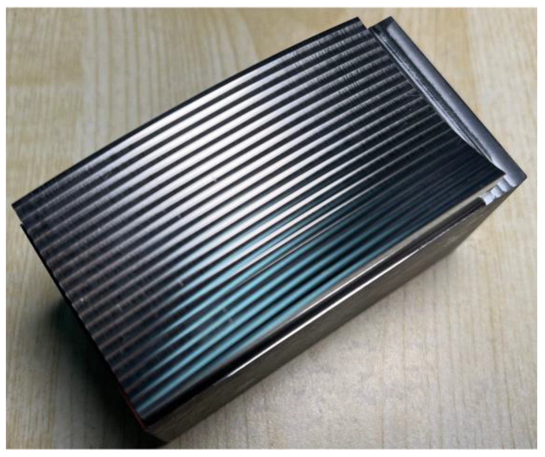
4.2. Milling a Free-Form Surface with Bull-Nose Cutter

In the present study, a bull-nose cutter with the same parameters as above was used in a machining experiment of a free-form surface obtained from the blade model. The CC path was generated according to the iso-parameters, the inclination angle was ${30}^{\circ }$, and the tilt angle was $0^{\circ }$ at any CC point. The spindle speed was 4000 rpm, and the feed rate per tooth was 0.03 mm/tooth. The workpiece’s material was 2Cr13, and the machined workpiece is shown in Figure 17.

After machining, the 2D profile of the workpiece was measured by a Mahr XT20. The 2D profile was also measured in three different directions and compared with the simulation results. The point $P_S\left(x=35.0,y=19.9,z=29.9\right)$ was selected as the starting point of the 2D profile measurement line in the workpiece coordinate system, and the endpoints were $P_{2,1}\left(x=35.0,y=32.0,z=30.6\right)$ and $P_{2,2}\left(x=42.0,y=27.9,z=30.1\right)$. Figure 18 shows the measurement and simulation results of the free-form surface. The blue line represents the measurement result of the plane surface along the direction, and the red line is for the simulation result. It can be observed that the measurement profiles are consistent with the simulation results along different measurement directions. It can be inferred that the proposed 2D contour can be effectively applied to free-form surfaces.

The obtained results show that the proposed 2D profile of five-axis CNC machining with a bull-nose cutter can be effectively applied to analyze free-form surface machining. The proposed 2D profile simulation model is expected to provide a reference for optimizing process parameters.

5. Conclusions

In the present study, a 2D profile simulation model is proposed for five-axis CNC machining with a bull-nose cutter. Based on the geometry and CL data of the machined workpiece, a simplified surface topography model is established. Based on the performed analyses, the main conclusions can be summarized as follows:

• The proposed model can be applied to accurately predict the 2D profile of the workpiece. This scheme can be extended to 3D profiles as well.
• The proposed model can be applied to predict the 2D profile of planes and free-form surfaces.
• Although this model is proposed for machining with bull-nose cutters, it can be extended to machining with other tools such as ball-end and drum tools.
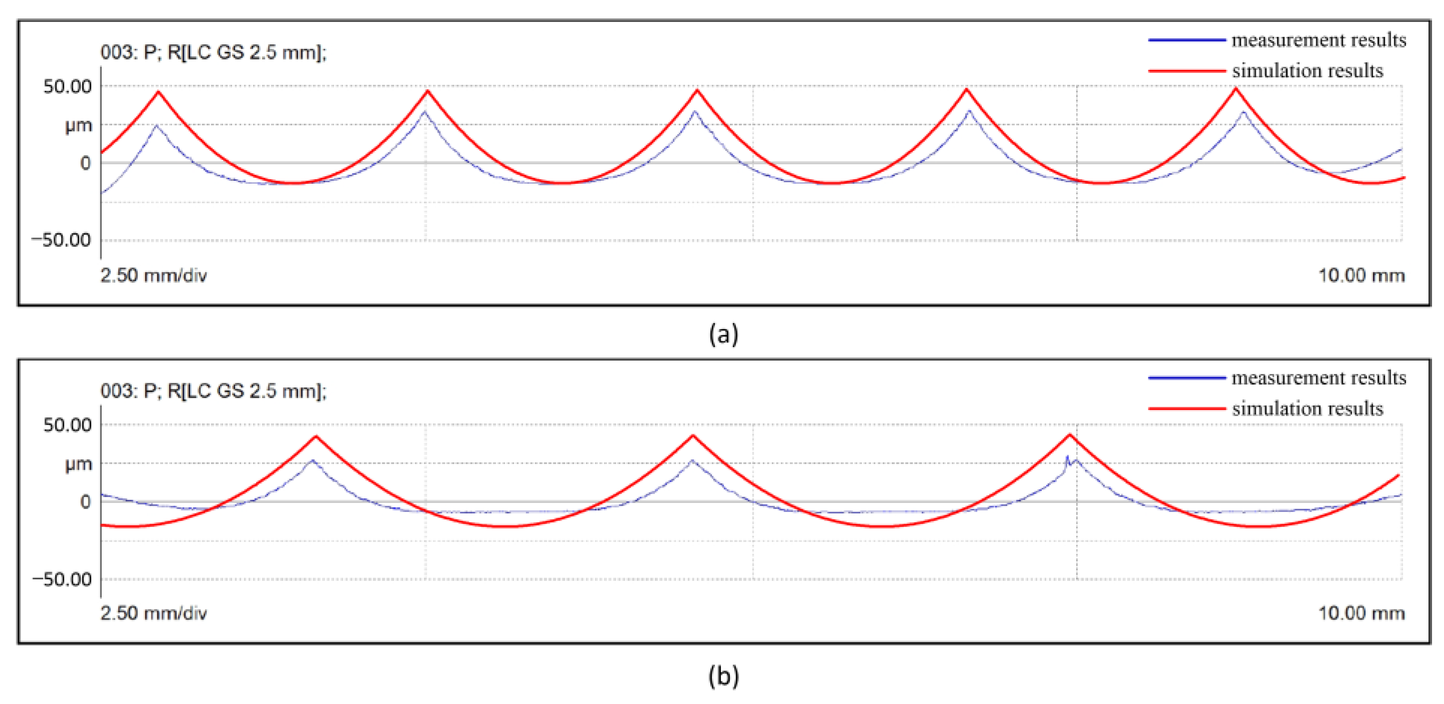
• Tool runout, wear, vibration, and other factors are ignored in the proposed model. However, these errors are inevitable in machining. Further, the phase angle between adjacent CC paths is not considered either. These may lead to error (no more than 20%) between the measurement and simulation results. Overall, the simulation results are consistent with the measurement experiments and can provide a reference for optimizing process parameters.

References

- Slătineanu, L.; Oşan, A.; Bănică, M.; Năsui, V.; Merticaru, V.; Mihalache, A.M.; Dodun, O.; Ripanu, M.I.; Nagit, G.; Coteata, M.; et al. Processing of convex complex surfaces with toroidal milling versus ball nose end mill. MATEC Web Conf. 2018, 178, 01003. [Google Scholar] [CrossRef]
- Davim, J.P. Machining of Complex Sculptured Surfaces; Springer: Berlin, Germany, 2012. [Google Scholar]
- Yao, C.; Tan, L.; Yang, P.; Zhang, D. Effects of tool orientation and surface curvature on surface integrity in ball end milling of TC17. Int. J. Adv. Manuf. Technol. 2018, 94, 1699–1710. [Google Scholar] [CrossRef]
- Lopes da Silva, R.H.; Hassui, A. Cutting force and surface roughness depend on the tool path used in side milling: An experimental investigation. Int. J. Adv. Manuf. Technol. 2018, 96, 1445–1455. [Google Scholar] [CrossRef]
- Toh, C.K. Cutter path orientations when high-speed finish milling inclined hardened steel. Int. J. Adv. Manuf. Technol. 2006, 27, 473–480. [Google Scholar] [CrossRef]
- Tan, L.; Yao, C.F.; Ren, J.X.; Zhang, D.H. Effect of cutter path orientations on cutting forces, tool wear, and surface integrity when ball end milling TC17. Int. J. Adv. Manuf. Technol. 2017, 88, 2589–2602. [Google Scholar] [CrossRef]
- de Souza, A.F.; Diniz, A.E.; Rodrigues, A.R.; Coelho, R.T. Investigating the cutting phenomena in free-form milling using a ball-end cutting tool for die and mold manufacturing. Int. J. Adv. Manuf. Technol. 2014, 71, 1565–1577. [Google Scholar] [CrossRef]
- Daymi, A.; Boujelbene, M.; Ben Amara, A.; Bayraktar, E.; Katundi, D. Surface integrity in high speed end milling of titanium alloy Ti-6Al-4V. Mater. Sci. Technol. 2011, 27, 387–394. [Google Scholar] [CrossRef]
- Yazid, M.Z.A.; Zainol, A. Tool life and surface roughness in dry high speed milling of aluminum alloy 7075-T6 using bull nose carbide insert. J. Eng. Sci. Technol. 2020, 15, 128–138. [Google Scholar]
- Yang, P.; Yao, C.; Xie, S.; Zhang, D.; Tang, D.X. Effect of Tool Orientation on Surface Integrity during Ball End Milling of Titanium Alloy TC17. In Proceedings of the Procedia CIRP, Stockholm, Sweden, 15–17 June 2016; pp. 143–148. [Google Scholar]
- Ko, T.J.; Kim, H.S.; Lee, S.S. Selection of the machining inclination angle in high-speed ball end milling. Int. J. Adv. Manuf. Technol. 2001, 17, 163–170. [Google Scholar] [CrossRef]
- Kalvoda, T.; Hwang, Y.R. Impact of various ball cutter tool positions on the surface integrity of low carbon steel. Mater Des. 2009, 30, 3360–3366. [Google Scholar] [CrossRef]
- Chen, X.X.; Zhao, J.; Dong, Y.W.; Han, S.G.; Li, A.H.; Wang, D. Effects of inclination angles on geometrical features of machined surface in five-axis milling. Int. J. Adv. Manuf. Technol. 2013, 65, 1721–1733. [Google Scholar] [CrossRef]
- Gdula, M. Empirical Models for Surface Roughness and Topography in 5-Axis Milling Based on Analysis of Lead Angle and Curvature Radius of Sculptured Surfaces. Metals 2020, 10, 932. [Google Scholar] [CrossRef]
- Khorasani, A.; Yazdi, M.R.S. Development of a dynamic surface roughness monitoring system based on artificial neural networks (ANN) in milling operation. Int. J. Adv. Manuf. Technol. 2017, 93, 141–151. [Google Scholar] [CrossRef]
- Oktem, H.; Erzurumlu, T.; Erzincanli, F. Prediction of minimum surface roughness in end milling mold parts using neural network and genetic algorithm. Mater Des. 2006, 27, 735–744. [Google Scholar] [CrossRef]
- Cao, L.; Huang, T.; Zhang, X.-M.; Ding, H. Generative Adversarial Network for Prediction of Workpiece Surface Topography in Machining Stage. IEEE-Asme Trans. Mechatron. 2021, 26, 480–490. [Google Scholar] [CrossRef]
- Moayyedian, M.; Mohajer, A.; Kazemian, M.G.; Mamedov, A.; Derakhshandeh, J.F. Surface roughness analysis in milling machining using design of experiment. SN Appl. Sci. 2020, 2, 1–9. [Google Scholar] [CrossRef]
- Dayan, G.M.; Kishore, R.H.; Praveen, V. Experimental investigation of cutting parameters in CNC machining for surface roughness, temperature and MRR for Ti alloys. Mater. Today 2019, 18, 2191–2196. [Google Scholar] [CrossRef]
- Kumar, S.; Singh, D.; Kalsi, N.S. Experimental Investigations of Surface Roughness of Inconel 718 under different Machining Conditions. Mater. Today 2017, 4, 1179–1185. [Google Scholar] [CrossRef]
- Layegh, K.S.E.; Lazoglu, I. 3D surface topography analysis in 5-axis ball-end milling. CIRP Ann. 2017, 66, 133–136. [Google Scholar] [CrossRef]
- Yuan, Y.J.; Jing, X.B.; Ehmann, K.F.; Zhang, D.W. Surface roughness modeling in micro end-milling. Int. J. Adv. Manuf. Technol. 2018, 95, 1655–1664. [Google Scholar] [CrossRef]
- Gao, T.; Zhang, W.H.; Qiu, K.P.; Wan, M. Numerical simulation of machined surface topography and roughness in milling process. J. Manuf. Sci. Eng. 2006, 128, 96–103. [Google Scholar] [CrossRef]
- Zhang, W.H.; Tan, G.; Wan, M.; Gao, T.; Bassir, D.H. A new algorithm for the numerical simulation of machined surface topography in multiaxis ball-end milling. J. Manuf. Sci. Eng. 2008, 130, 11. [Google Scholar] [CrossRef]
- Yujun, C.; Lizhen, P. A geometrical simulation of ball end finish milling process and its application for the prediction of surface topography. In Proceedings of the 2010 International Conference on Mechanic Automation and Control Engineering, Wuhan, China, 26–28 June 2010; pp. 519–522. [Google Scholar]
- Peng, Z.; Jiao, L.; Yan, P.; Yuan, M.; Gao, S.; Yi, J.; Wang, X. Simulation and experimental study on 3D surface topography in micro-ball-end milling. Int. J. Adv. Manuf. Technol. 2018, 96, 1943–1958. [Google Scholar] [CrossRef]
- Wei, J.; Hou, X.; Sun, C. Modeling and simulation of surface topography in five-axis ball end milling. J. Phys. Conf. Ser. 2021, 1820, 012049. [Google Scholar] [CrossRef]
- Quinsat, Y.; Lavernhe, S.; Lartigue, C. Characterization of 3D surface topography in 5-axis milling. Wear 2011, 271, 590–595. [Google Scholar] [CrossRef]
- Wang, B.; Zhang, Q.; Wang, M.H.; Zheng, Y.H.; Kong, X.J. A predictive model of milling surface roughness. Int. J. Adv. Manuf. Technol. 2020, 108, 2755–2762. [Google Scholar] [CrossRef]
- Zhou, R.; Chen, Q. An analytical prediction model of surface topography generated in 4-axis milling process. Int. J. Adv. Manuf. Technol. 2021, 115, 3289–3299. [Google Scholar] [CrossRef]
- Lavernhe, S.; Quinsat, Y.; Lartigue, C. Model for the prediction of 3D surface topography in 5-axis milling. Int. J. Adv. Manuf. Technol. 2010, 51, 915–924. [Google Scholar] [CrossRef]
- Bizzarri, M.; Lávička, M. A symbolic-numerical approach to approximate parameterizations of space curves using graphs of critical points. J. Comput. Appl. Math. 2013, 242, 107–124. [Google Scholar] [CrossRef]
- Barton, M.; Bizzarri, M.; Rist, F.; Sliusarenko, O.; Pottmann, H. Geometry and tool motion planning for curvature adapted CNC machining. Acm. T Graph. 2021, 40, 1–16. [Google Scholar] [CrossRef]