Hybrid VOF–Lagrangian CFD Modeling of Droplet Aerobreakup

Abstract

A hybrid VOF–Lagrangian method for simulating the aerodynamic breakup of liquid droplets induced by a traveling shock wave is proposed and tested. The droplet deformation and fragmentation, together with the subsequent mist development, are predicted by using a fully three-dimensional computational fluid dynamics model following the unsteady Reynolds-averaged Navier–Stokes approach. The main characteristics of the aerobreakup process under the shear-induced entrainment regime are effectively reproduced by employing the scale-adaptive simulation method for unsteady turbulent flows. The hybrid two-phase method combines the volume-of-fluid technique for tracking the transient gas–liquid interface on the finite volume grid and the discrete phase model for following the dynamics of the smallest liquid fragments. The proposed computational approach for fluids engineering applications is demonstrated by making a comparison with reference experiments and high-fidelity numerical simulations, achieving acceptably accurate results without being computationally expensive.

1. Introduction

Due to the continuous advancement in computing power and technology, computational fluid dynamics (CFD) has become an established industrial design tool, which helps to reduce design times and improve fluids engineering processes [1]. The present CFD study deals with a particular industrial fluid dynamics problem that has several very important applications, namely, the aerodynamic breakup of liquid droplets under shock wave loading, which is commonly referred to as aerobreakup [2]. The exposure to the high-speed post-shock airflow is responsible for the drift, distortion, and breakup of the original droplet into much smaller fragments [3]. This phenomenon has a crucial role in many fluids engineering applications including, just to mention, raindrop fragmentation in the flow field around supersonic aircrafts. Indeed, in the aerospace industry, a proper aerodynamic design can help greatly reduce the erosion caused by the impingement of small liquid fragments at high relative speeds on the aircraft surfaces [4].

Theoretically, the physics of aerobreakup is controlled by the Ohnesorge number (Oh) of the droplet, which compares the effects of liquid viscosity and surface tension, and the Weber number (We) at freestream conditions, which describes the ratio of disruptive inertial to restorative interfacial forces. Previously, based on the definition of various different breakup modes, the interpretation and identification of the aerobreakup mechanism have been recently reviewed and simplified by Theofanous, who introduced only two principal modes of fragmentation that are based on the underlying physical mechanism of the dominant interfacial instabilities [5]. Basically, at low Ohnesorge numbers ($\mathrm{Oh}\ll 1$), the process is practically governed by the Weber number. For low Weber numbers ($10<\mathrm{We}<{10}^2$), the Rayleigh–Taylor (RT) instability represents the main driving mechanism for the aerobreakup, which is referred to as the RT piercing regime, corresponding to a moderate fragmentation. Differently, at high Weber numbers ($\mathrm{We}>{10}^3$), the breakup process is governed by the Kelvin–Helmholtz instability of the stretched liquid filaments that are formed at the periphery of the deforming droplet, with the subsequent liquid sheet stripping and thinning, and the extended entrainment of liquid mist. This terminal mechanism, which is referred to as the shear-induced entrainment (SIE) regime, corresponds to a strong fragmentation, where capillary forces and turbulent mixing play an important role [2].

Several experimental studies have been conducted to investigate the relevant physical mechanisms and the main features of the droplet aerobreakup. In practical experiments, a traveling planar shock front is often reproduced through shock tube devices, where uniform airflow conditions are established around the water body [6]. In these experiments, sophisticated visualization techniques are used to analyze the deformation and breakup of droplets under shock wave loading [7]. In particular, the physical mechanisms determining the dynamics of the dispersed particles that are forming as a result of the chaotic fragmentation in the SIE regime have been investigated by different research groups [8,9]. However, the experimental quantification of the characteristic sizes and velocities of the liquid fragments inside the mist remains very challenging.

From a numerical point of view, since the droplet aerobreakup under the SIE regime is characterized by a very broad range of spatial and temporal scales, the accurate prediction of the droplet deformation and fragmentation is particularly demanding in terms of computing power. Due to the high computational cost of fully three-dimensional (3D) simulations, several CFD studies have been conducted in two spatial dimensions, by considering that the shear-induced breakup of a cylindrical liquid column [10,11,12]. Two-dimensional simulations have been mostly focused on the early stages of the breakup process, without investigating the droplet fragmentation and the subsequent mist development [13,14]. On the other hand, to make them affordable in the context of preliminary analyses, 3D computations have been most often conducted by solving the Euler equations, while neglecting the viscous effects [15,16]. Typically, compressible two-phase solvers based on a five-equation model [17] are used to computationally study shock–droplet interactions, where the gas–liquid interface is modeled using the volume-of-fluid (VOF) approach [18]. The governing equations consist of two continuity equations for the two different phases, the volume fraction advection equation, and the mixture momentum and energy equations. As far as turbulence modeling is concerned, either the under-resolved direct numerical simulation (DNS) or the large eddy simulation (LES) approach is usually followed [6,16]. However, these expensive CFD models are generally limited to the early stages of the aerobreakup process, investigating the droplet surface instabilities, without examining the later-stages fragmentation and the liquid mist evolution.

The main goal of the present work is the computational evaluation of the droplet aerobreakup under the SIE regime following a relatively lighter approach, where the viscous effects are not neglected. To investigate the multiscale features of the phenomenon with a viable computational cost, the mean turbulent flow field is simulated by solving the compressible unsteady Reynolds-averaged Navier–Stokes (URANS) equations endowed with a two-equation turbulence model. In contrast to our previous work [19], the newly proposed URANS model is supplied with the scale-adaptive simulation (SAS) method for unsteady turbulent flows [20]. Being able to dynamically adjust to the resolved unsteady turbulent structures, the SAS-URANS model represents an attractive alternative to the existing expensive numerical methods for transient two-phase flows. Moreover, the CFD modeling approach is enriched by introducing a Lagrangian method for tracking the sub-particles that originate from the breaking droplet. The simulations are conducted with the commercial solver Ansys Fluent, which is widely used for industrial CFD applications [1,21]. The mean-flow-governing equations are solved employing a finite volume (FV) numerical technique [13,22], where the transient tracking of the air–water interface is approximated through the VOF methodology.

Basically, a hybrid two-phase model combining the VOF approach and the discrete phase model (DPM) is implemented in the CFD solver, with the former model tracking the gas–liquid interface to describe the deformation and fragmentation of the parent body, and the latter model allowing for tracking the child particles. The combination of CFD with DPM represents a powerful tool to simulate two-phase flows of engineering interest, which has recently received considerable attention. For instance, the analysis of a combined CFD-DPM method for predicting the performance of finely atomized sprays for dust suppression has been performed in [23], while a two-stage multi-phase model for close-coupled gas atomization has been developed in [24], by combining an Eulerian model for primary atomization and a Lagrangian particle tracking approach to predict the particle size distribution resulting from secondary atomization. Following a similar but different approach, a VOF-to-DPM model has been recently employed for the under-resolved DNS of the aerodynamic droplet breakup in [11]. In the present work, instead, the combined VOF–Lagrangian model is developed and tested in the framework of the SAS-URANS approach. The overall computational modeling procedure for simulating the droplet aerobreakup is validated against reference data that are provided by both experimental studies [8] and high-fidelity numerical simulations [15].

The rest of this manuscript is organized as follows. After describing the hybrid VOF–Lagrangian approach in Section 2, the applied CFD model is introduced in Section 3. The results of the computational analysis are presented and discussed in Section 4. Finally, in Section 5, some concluding remarks are drawn.

2. Hybrid VOF–Lagrangian Approach

Together with the droplet drift and deformation, the passage of a shock wave front leads to the fragmentation of a large portion of the liquid body. Indeed, the parent droplet is partially converted into much smaller child droplets, whose size can also result in being comparable to the local mesh size that is used by numerical investigations. Differently from [19], where only the early stages of the interaction process were examined, the hybrid VOF–Lagrangian two-phase CFD model that is used in this work enables us to simulate the droplet aerobreakup also during the later phase.

2.1. VOF Method

To approximate the transient air–water interface, while tracking it on the FV mesh, the classical VOF method is utilized. This technique was demonstrated to be very efficient when dealing with the complex interface between two immiscible fluids [18] and has been widely used to investigate the droplet aerobreakup [6,13]. The additional field variable $\alpha$ that represents the volume fraction of liquid is introduced, which changes discontinuously across the interface. Following this approach, the compressible Navier–Stokes equations are solved for an effective mixture fluid, whose (averaged) properties are determined by the actual volume fractions. For instance, the mixture density and molecular viscosity are defined as:

$$\rho =\alpha {\rho }_{\mathrm{l}}+(1-\alpha ){\rho }_{\mathrm{g}},$$

(1)

and

$$\mu =\alpha {\mu }_{\mathrm{l}}+(1-\alpha ){\mu }_{\mathrm{g}},$$

(2)

respectively, where the subscripts denote liquid and gas phases.

The volume fraction $\alpha$ is calculated throughout the computational domain by solving a simple advection equation, that is:

$$\frac{\partial \left(\alpha {\rho }_{\mathrm{l}}\right)}{\partial t}+\nabla ·\left(\alpha {\rho }_{\mathrm{l}}\mathbf{u}\right)=0.$$

(3)

Therefore, the main advantage of the VOF method is that the liquid mass is correctly conserved for any given mesh resolution, which is particularly important for the present URANS approach. As the non-physical smearing of the interface due to numerical diffusion leads to a loss of accuracy in the definition of the interface location, the sharp interface modeling type, along with interfacial antidiffusion, was used [16]. Another interface-capturing method that is frequently employed when simulating the droplet aerobreakup is the level-set (LS) method [25]. The advantage of the LS approach is that it provides a sharp definition of the interface, but it is not mass conservative and thus requires higher-order numerical schemes [26]. To more accurately predict the air–water interface, the application of the coupled LS and VOF method, which combines the advantages of both methods, is currently under study.

In the VOF framework, the effect of surface tension forces at the air–water interface can be simply simulated by employing the continuum surface force model proposed in [27], where the momentum equation is supplied with an additional source term due to surface tension [28]. The present VOF method for simulating the mixture fluid dynamics is supplemented with a Lagrangian approach for particle tracking as discussed in the following.

2.2. Discrete Phase Model

The so-called VOF-to-DPM method implemented in the industrial CFD solver that is utilized in this study allows for automatic switching from the above VOF approach to a Lagrangian model for approximating the dynamics of the sub-droplets that are stripped from the main droplet [29]. Depending on the local flow conditions, where it is appropriate, the liquid volume fraction of the FV cell is converted into liquid particles, while an equal volume of gas is created to maintain the volume conservation in the same cell. The possible transition is controlled by a couple of user-defined parameters related to both size and shape of the water fragments originating from the breakup process. The first parameter corresponds to the diameter of the volume-equivalent sphere, which needs to be within a specified range. The second parameter corresponds to the so-called asphericity, which stands for a normalized measure of the shape deviation from that spherical one. For the present simulations, the maximum equivalent diameter is chosen corresponding to a spherical domain occupying eight times the volume of an interface cell, while the threshold of $0.5$ is prescribed for the maximum asphericity. Practically, only water fragments obeying these two criteria are converted into liquid particles. Note that the VOF-to-DPM transition tool is directly combined with dynamic mesh adaption following the mixture fluid evolution [30].

Once originated, the discrete phase is simulated by tracking the particles that evolve in the continuous flow field, while imposing the momentum balance on each particle. Namely, given the position ${\mathbf{x}}_p\left(t\right)$ and the velocity ${\mathbf{u}}_p=d{\mathbf{x}}_p/dt$ of a generic particle, the corresponding trajectory is calculated by integrating the following momentum equation (per unit particle volume):

$${\rho }_{\mathrm{l}}\frac{d{\mathbf{u}}_p}{dt}={\rho }_{\mathrm{l}}{f}_{\mathrm{d}}\left(\mathbf{u}-{\mathbf{u}}_p\right)+\left({\rho }_{\mathrm{l}}-\rho \right)\mathbf{g}.$$

(4)

The two terms at the right-hand-side of (4) represent the aerodynamic drag and the gravity forces, whereas the residual forces exerted on the particle (for instance, the virtual mass force) are considered negligible. The aerodynamic drag force is determined by fixing:

$$f_{\mathrm{d}}=\frac{18\mu }{{\rho }_{\mathrm{l}}{d}_p^2}\frac{C_d{\mathrm{R}\mathrm{e}}_p}{24},$$

(5)

where ${\mathrm{R}\mathrm{e}}_p=\rho \left|\mathbf{u}-{\mathbf{u}}_p\right|d_p/\mu$ stands for the particle Reynolds number, and $C_d$ is the drag coefficient. The latter parameter is evaluated as a known function of ${\mathrm{Re}}_p$, according to the experimental relationship derived in [31] for spherical particles. Due to the Lagrangian approach, micro-droplet properties such as equivalent diameter, position, and velocity can be statistically determined for the ongoing simulation.

3. CFD Modeling

In this section, after introducing the particular case flow under investigation, the main characteristics of the CFD model are presented, including the turbulence closure procedure. Differently from similar numerical studies solving the Euler equations, our engineering analysis employs the compressible Navier–Stokes equations, by also taking into account the surface tension effects at the air–water interface.

3.1. Flow Configuration

The flow geometry practically reproduces a shock tube device with a square cross-section, where the spatial coordinates system $(x,y,z)$ is chosen with the first axis direction along the tube axis, corresponding to the traveling direction of the shock front. Based on previous numerical studies conducted for similar flow configurations, the extent of the computational domain is chosen such that $-30<x/d_0<40$, $\left|y\right|/d_0<30$. and $\left|z\right|/d_0<30$, where $d_0=4.8$ mm stands for the initial diameter of the water sphere. The current droplet size represents one of the most studied cases, corresponding to the classical experiments of Igra and Takayama [7]. The above domain size serves as the necessary compromise between numerical accuracy and computational costs, as it could be determined by industrial researchers and developers. Following previous works, this size of the computational domain can be considered sufficiently large to avoid non-physical wave reflections on the boundaries [32].

In this study, differently from [19], the shock tube flow is not explicitly simulated, but the discontinuous air flow conditions are directly imposed. Practically, the experimental conditions are mimicked by initially setting two different thermodynamic states for the air occupying the two different subdomains that are separated by a virtual cross diaphragm perpendicular to the x-axis. The simulations are initiated with the shock front being positioned one diameter away from the droplet center, while the origin of the coordinate system corresponds to the initial position of the droplet leading edge. Practically, given the atmospheric pre-shock conditions in a section, the high-speed post-shock conditions in the other one uniquely correspond to the prescribed Mach number. The latter parameter was selected as $\mathrm{Ma}=1.47$, representing one of the cases mostly investigated in the engineering and scientific literature, both computationally [10,15] and experimentally [7]. As it is empirically demonstrated, the proposed model can reproduce a plane shock wave traveling at the prescribed velocity that is $V_{\mathrm{S}}=505$ m/s. For brevity, the airflow parameters corresponding to the present simulations are summarized in

Table 1. Airflow parameters.

Parameter	Pre-Shock	Post-Shock
Temperature (K)	293	381
Pressure (kPa)	101.3	239
Density (kg/m${}^3$)	1.204	2.18
Viscosity (Pa s)	$1.8\times {10}^{-5}$	$2.2\times {10}^{-5}$
Velocity (m/s)	0	226
Mach number	0	0.577

. It is worth noting that owing to the actual post-shock thermodynamic conditions, the ambient air pressure results in being greater than the saturation pressure of water, and thus, the liquid body does not undergo a phase change. In practice, the two different fluids can be considered immiscible, which could be no more valid for increasing Mach number.

The density and the dynamic viscosity of the liquid phase are initially set to ${\rho }_{\mathrm{l}0}=998$ kg/m${}^3$ and ${\mu }_{\mathrm{l}0}=1.00\times {10}^{-3}$ Pa s, while the surface tension at the gas–liquid interface is assumed equal to $\sigma =7.29\times {10}^{-2}$ N/m. This way, the characteristic Ohnesorge and Weber numbers result in being $\mathrm{Oh}={\mu }_{\mathrm{l}0}/\sqrt{{\rho }_{\mathrm{l}0}\sigma d_0}=1.64\times {10}^{-4}$ and $\mathrm{We}={\rho }_{\mathrm{g}}{u}_{\mathrm{g}}^2{d}_0/\sigma =7.3\times {10}^3$, respectively. According to these values, the present configuration corresponds to the droplet aerobreakup under the SIE regime [8]. Moreover, based on the high Weber number, as well as the high Reynolds number, that is, $\mathrm{Re}={\rho }_{\mathrm{g}}{u}_{\mathrm{g}}{d}_0/{\mu }_{\mathrm{g}}=1.06\times {10}^5$, both capillary and viscous effects might be neglected in practical calculations. Indeed, similar numerical studies have been mostly conducted by solving the compressible Euler equations without including the surface tension term [15]. For the sake of completeness, these effects are not ignored in the present study involving the Navier–Stokes equations, paving the way for a more general CFD modeling approach.

Finally, the system of governing equations is completed by employing two equations of state for the two different fluids. Together with the ideal gas law, the following equation is applied for the liquid phase [33]:

$$\frac{{\rho }_{\mathrm{l}}}{{\rho }_{\mathrm{l}0}}={\left(\frac{p+\mathcal{B}}{p_0+\mathcal{B}}\right)}^{\frac{1}{\kappa }},$$

(6)

where $p_0$ and ${\rho }_{\mathrm{l}0}$ represent the reference pressure and density levels, while $\mathcal{B}$ and $\kappa$ are constant parameters. Following [13], the pressure-like parameter $\mathcal{B}$ and the so-called adiabatic index $\kappa$ are set to the values of 305 MPa and $6.68$, respectively. Noteworthily, given the maximum pressure level achieved in the practical simulations, the water density can be considered approximately constant for the present engineering analysis.

3.2. Turbulence Modeling

The turbulence effects become significant under supersonic flow conditions, playing an important role in the breakup of the smallest sub-droplets [32]. In this CFD study, the unsteady mean turbulent flow around the droplet is numerically predicted by solving the URANS equations with the scale-adaptive simulation (SAS) method [20]. The SAS-URANS approach is based on the shear-stress transport (SST) k–$\omega$ turbulence model [34], where two additional transport equations are solved for the turbulent kinetic energy and the specific turbulent dissipation rate. Among the different versions of the k–$\omega$ model, the SST formulation represents the most commonly used in engineering research given its high accuracy-to-expense ratio. This model provides a better prediction of separated flows, having the ability to account for the transport of the principal shear stress in adverse pressure gradient boundary layers. In the SAS framework, an extra production term is added in the $\omega$ equation, which is sensitive to resolved unsteady fluctuations. Contrary to the standard SST k–$\omega$ model adopted in [19], the present SAS formulation provides a turbulent length scale that is depending on the local flow structure. Practically, the method allows for resolving unsteady turbulence structures with LES-like accuracy, where it is appropriate, and is particularly suitable for flows with strong instabilities [35]. In addition, the $\gamma$ transition model is used in conjunction with the SST model, where an additional transport equation is solved for the so-called turbulence intermittency [36].

Due to these features, the SAS-URANS method, which is increasingly used by industrial researchers, results in being particularly suitable for simulating the complex unsteady two-phase flow under investigation. For the sake of brevity, the mean-flow-governing equations, including the model equations, are not reported here and can be found in the referenced works.

3.3. CFD Solver

The numerical simulations are conducted by using the industrial solver Ansys Fluent, which has been successfully employed for droplet breakup investigations [12,14], as well as in applied CFD studies of bluff body flows by the present research group [21]. The solver utilizes the finite volume (FV) method to approximate the compressible flow, with the conservation principles being applied over each control volume [37,38]. To accurately model the two-phase flow, both high-order spatial and time discretization schemes are employed. Specifically, the pressure–velocity coupling is addressed using the pressure implicit with the splitting of operators (PISO) scheme [39], which is commonly adopted for complex transient flows. As to spatial discretization, the pressure staggering option is used for the pressure field, the bounded-central differencing scheme is employed for the momentum equation, while the QUICK scheme [40] is adopted for the continuity and energy equations, as well as for the additional turbulence model equations. The compressive discretization scheme is used to solve the volume fraction advection Equation (3). As far as time integration is concerned, a second-order implicit method is used along with the VOF implicit scheme, while prescribing a low time step size, which is $\mathsf{\Delta }t=2\times {10}^{-7}$ s, due to the restrictions of convection, diffusion, and surface tension effects.

The practical computational domain corresponds to the entire physical domain described above, without imposing any symmetry condition at the midplane, as was performed in [19]. This way, fully three-dimensional simulations are conducted. Pressure inlet and pressure outlet boundary conditions are associated with the sub-domains corresponding to the post-shock and pre-shock air conditions, respectively. The adaptive mesh resolution ranges from 30 to 100 cells per original droplet diameter, with the finest mesh being used in the transition region between the two phases, as the total number of FV cells results in being about 10 million. The choice of this mesh resolution is based on our previous studies [14,19], where a grid sensitivity analysis was completed. It is worth noting that the finest mesh size is comparable to that one recently used for under-resolved DNS in [15]. Nevertheless, the two approaches are completely different. Therein, a direct solution of the Euler equations was performed, where the numerical scheme inherently included artificial viscosity mimicking the effect of unresolved scales, without introducing any closure model. Very dissimilarly, the present study aims to determine the mean turbulent flow by solving the URANS equations supplied with a suitable turbulence model.

4. Results

Starting from the initial conditions discussed in Section 3.1, the planar shock front actually travels in the positive x-axis direction, impacting the water sphere at $t_0=0.5d_0/V_{\mathrm{S}}$. The robustness of the proposed CFD model and the accuracy of the unsteady solution have been preliminarily assessed through comparison with the theoretical discontinuous profiles of the flow field variables, similarly to what was performed in [19]. In the following, as is commonly found in droplet aerobreakup studies, the independent time variable is nondimensionalized as follows:

$$t^{*}=\frac{u_{\mathrm{g}}}{d_0\sqrt{\epsilon }}(t-t_0),$$

(7)

where $\epsilon$ stands for the ratio between liquid and gas densities.

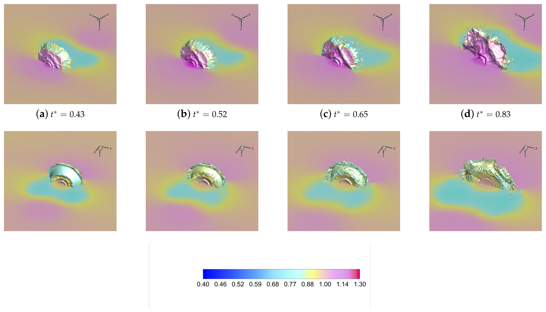
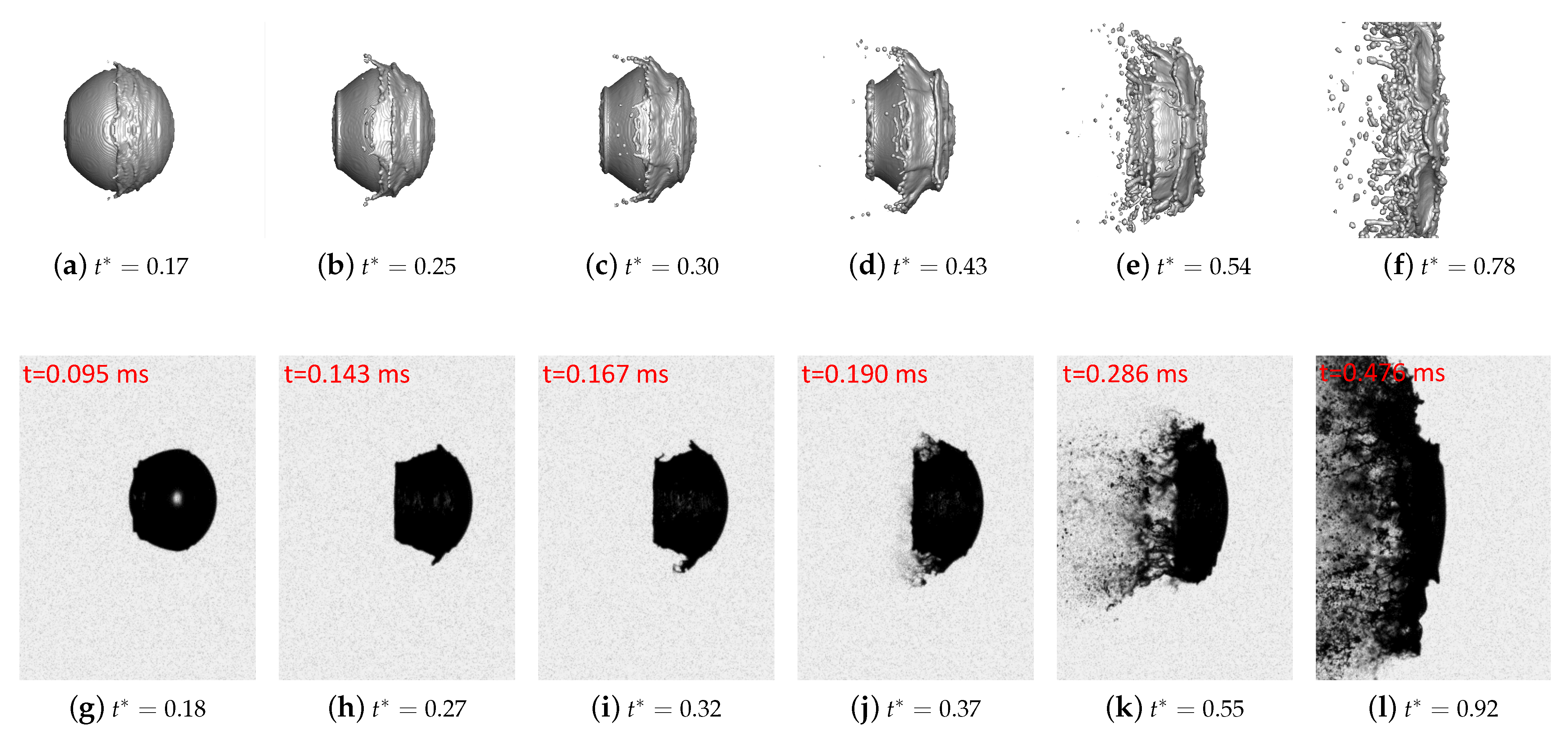
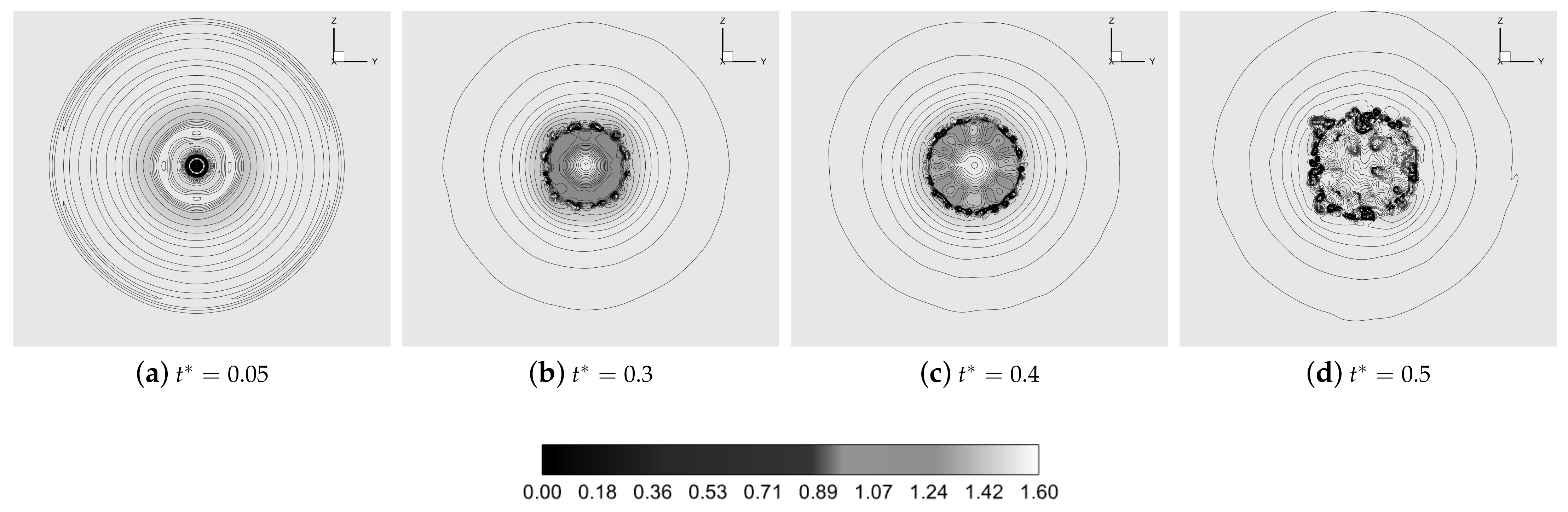
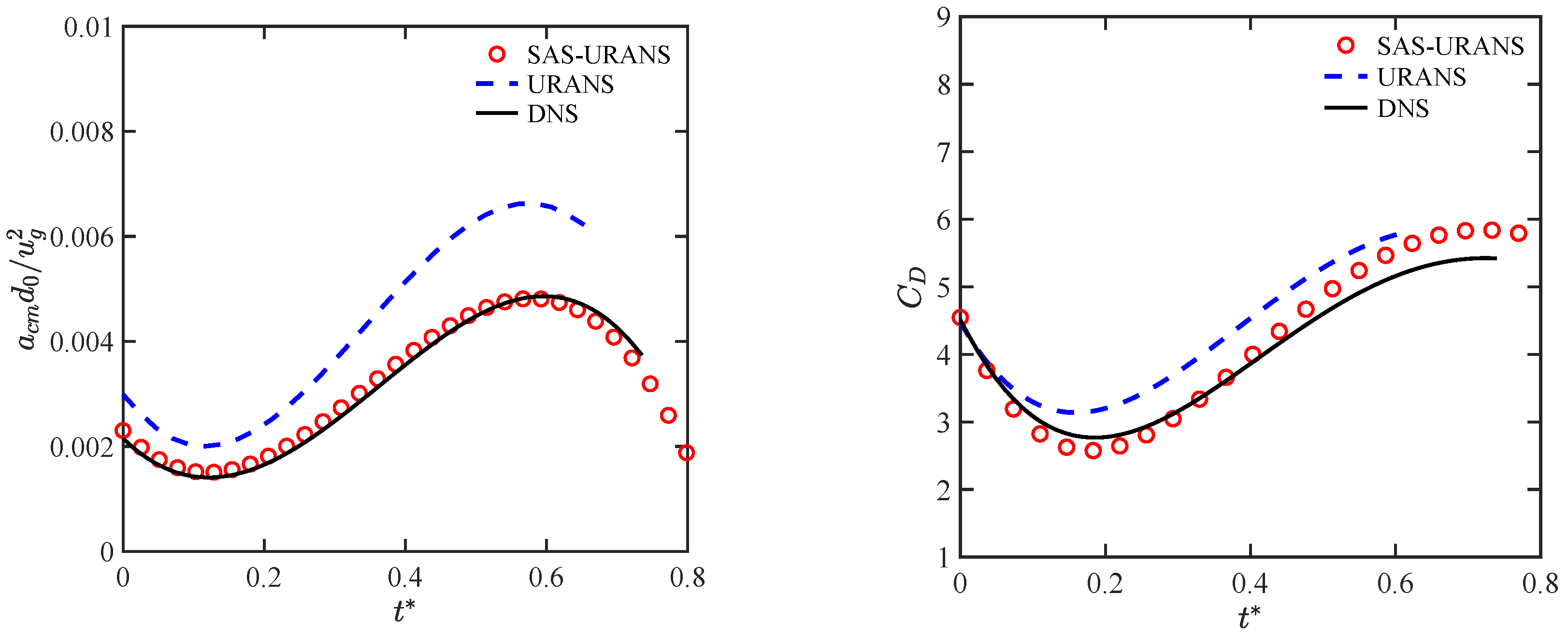
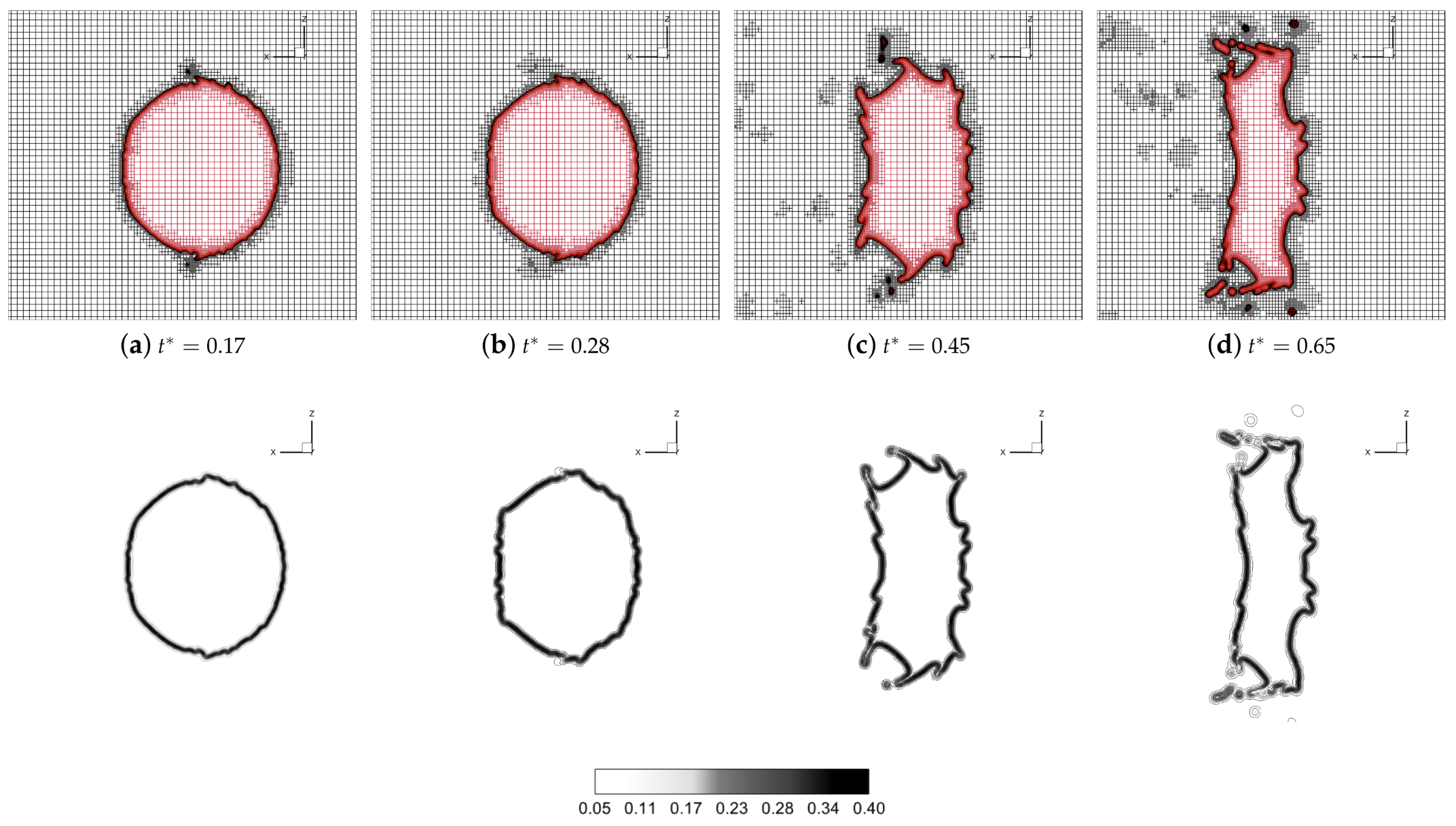
4.1. Droplet Deformation

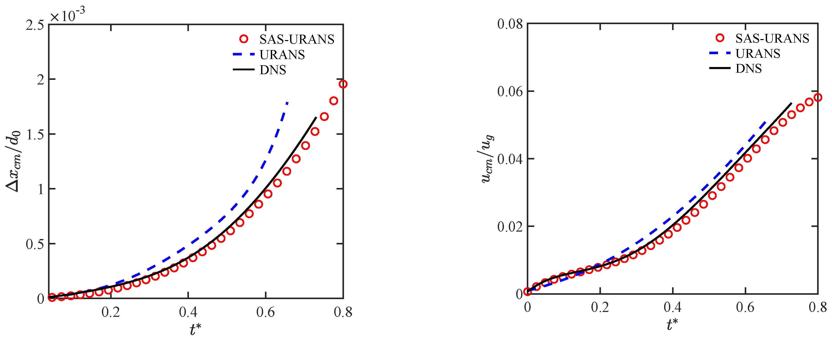
As a consequence of the exposure to the post-shock high-speed flow, after the reaction time has elapsed, during which the solution practically corresponds to the flow past a rigid sphere, the deformation of the droplet begins to be observed. At the early stages of the process, following the small-scale instabilities originating on the liquid surface, the water body is flattened in the streamwise direction. That is mainly due to the high pressure difference between the front and back droplet sides. The droplet evolution is illustrated, in Figure 1 and Figure 2, by drawing the isosurfaces of the volume fraction of water at $\alpha =0.5$, to identify the droplet boundary, along with the instantaneous pressure contours at the midplane $y=0$. Both front and back views are reported, for eight typical instants in the time interval $0.044\le t^{*}\le 0.83$, with the pressure field being normalized by the post-shock freestream value. To correctly illustrate the droplet drift and deformation, the size and position of the zoomed images are the same for each snapshot of these two figures. Initially, as the droplet shape changes very slightly, both reflected and transmitted wavefronts are apparent in Figure 1. Then, the formation of ligaments at the droplet surface is observed, which are further stretched and, eventually, disintegrated by the aerodynamic shearing force of the surrounding airflow, as shown in Figure 2. The water body is continuously eroded, with sub-droplets being stripped from the parent droplet, as well as from the water ligaments. In the later stages, the liquid droplet shatters into smaller fragments distributed widely in the flow field. These pictures confirm the qualitative features of the so-called shear stripping breakup mechanism, which is typical at high Weber numbers, under the SIE regime [2].

To further analyze the CFD solution, in Figure 3, the vortical structures are visualized by plotting the contours of the second component of the normalized vorticity vector field in the midplane $y=0$, as well as on the droplet boundary. The equatorial recirculation region that is formed around the droplet is apparent, corresponding to the muffin-like shape of the deforming water body. As observed in [15], this leads to the formation of liquid sheets that are simultaneously drawn out from the hemispherical lip and the planar back of the droplet. When making a comparison with URANS [19], the present SAS-URANS method allows for a better representation of unsteady turbulent flow features, with the capture of some fine-scale structures.

In Figure 4, the morphology of the deforming droplet is demonstrated by showing the side view of the water body traced by nondimensional time, making a direct comparison with the experimental images provided by Theofanous and co-workers [8]. The simulation results partially agree with the observations made in the experiment investigating the water droplet breakup at $\mathrm{We}=7.8\times {10}^2$ with a post-shock flow Mach number of $0.32$. In the CFD analysis, owing to the higher Mach number, the surface instability at the equator is more pronounced than that one originating at the rear part of the body. The comparison with experimental findings is initially quite good while, at later times, the URANS solution inherently cannot represent the fine scale structure of the two-phase flow. Nevertheless, these results suggest that the SAS formulation is capable of accurately reproducing the transition process by resolving, at least partially, the small-scale flow structures at the gas–liquid interface. In practice, the proposed multiscale URANS approach is found to predict the early stage breakup mechanisms with an accuracy comparable to more expensive methods.

The good performance of the present CFD model is further demonstrated by examining the partial density field of the gas phase, normalized by the post-shock freestream value, whose contour plots are depicted in Figure 5, in the plane corresponding to the initial position of the droplet trailing edge, at four typical time instants. Also due to the fully three-dimensional character of the SAS-URANS solution, some important features of the air flow field that are related to developing RT instabilities can be observed. The gas density field, which is initially axisymmetric, at later time instants shows the characteristic transverse azimuthal modulations observed in the DNS study [15]. Later on, the solution evolves into a turbulent wake flow. This capability represents a distinctive feature of the proposed modeling approach, which makes it different from recent similar numerical studies investigating the droplet aerobreakup at comparable Mach number [11]. Therein, only a very limited fraction of the flow field was simulated, while applying periodic boundary conditions in the azimuthal direction. This limitation undoubtedly affected the predictions of droplet deformation and breakup due to vortex shedding and turbulence.

4.2. Droplet Drift

The quantitative validation of the present CFD model is addressed by examining the kinematics of the droplet center-of-mass (CM), while making a comparison with reference DNS data [15]. The time-dependent axial position and velocity of the CM are determined according to:

$$x_{\mathrm{cm}}\left(t\right)=\frac{1}{m_{\mathrm{l}}}{\int }_{\mathsf{\Omega }}\alpha {\rho }_{\mathrm{l}}xd\mathsf{\Omega },u_{\mathrm{cm}}\left(t\right)=\frac{1}{m_{\mathrm{l}}}{\int }_{\mathsf{\Omega }}\alpha {\rho }_{\mathrm{l}}ud\mathsf{\Omega },$$

(8)

where $\mathsf{\Omega }$ represents the overall computational domain, and $m_{\mathrm{l}}={\int }_{\mathsf{\Omega }}\alpha {\rho }_{\mathrm{l}}d\mathsf{\Omega }$ is the constant liquid mass in the domain. Owing to the VOF formulation, the above evaluations inherently take into account the proper contribution from regions occupied by the liquid phase.

The displacement and velocity of the droplet CM are reported in Figure 6, while the approximated acceleration and the corresponding drag coefficient are drawn in Figure 7. The unsteady acceleration $a_{\mathrm{cm}}$ is simply evaluated by numerically differentiating the velocity data while, following [41], an attempt to evaluate the time-dependent drag force coefficient is made by simply defining:

$$C_D=\frac{m_{\mathrm{l}}{a}_{\mathrm{cm}}}{\frac{1}{2}{\rho }_{\mathrm{g}}{(u_{\mathrm{g}}-u_{\mathrm{cm}})}^2{A}^{\prime }}$$

(9)

where A stands for the initial frontal area of the liquid droplet. When making a comparison with previous URANS solution [19], the novel SAS formulation results in being more accurate, as the reference DNS is clearly approached.

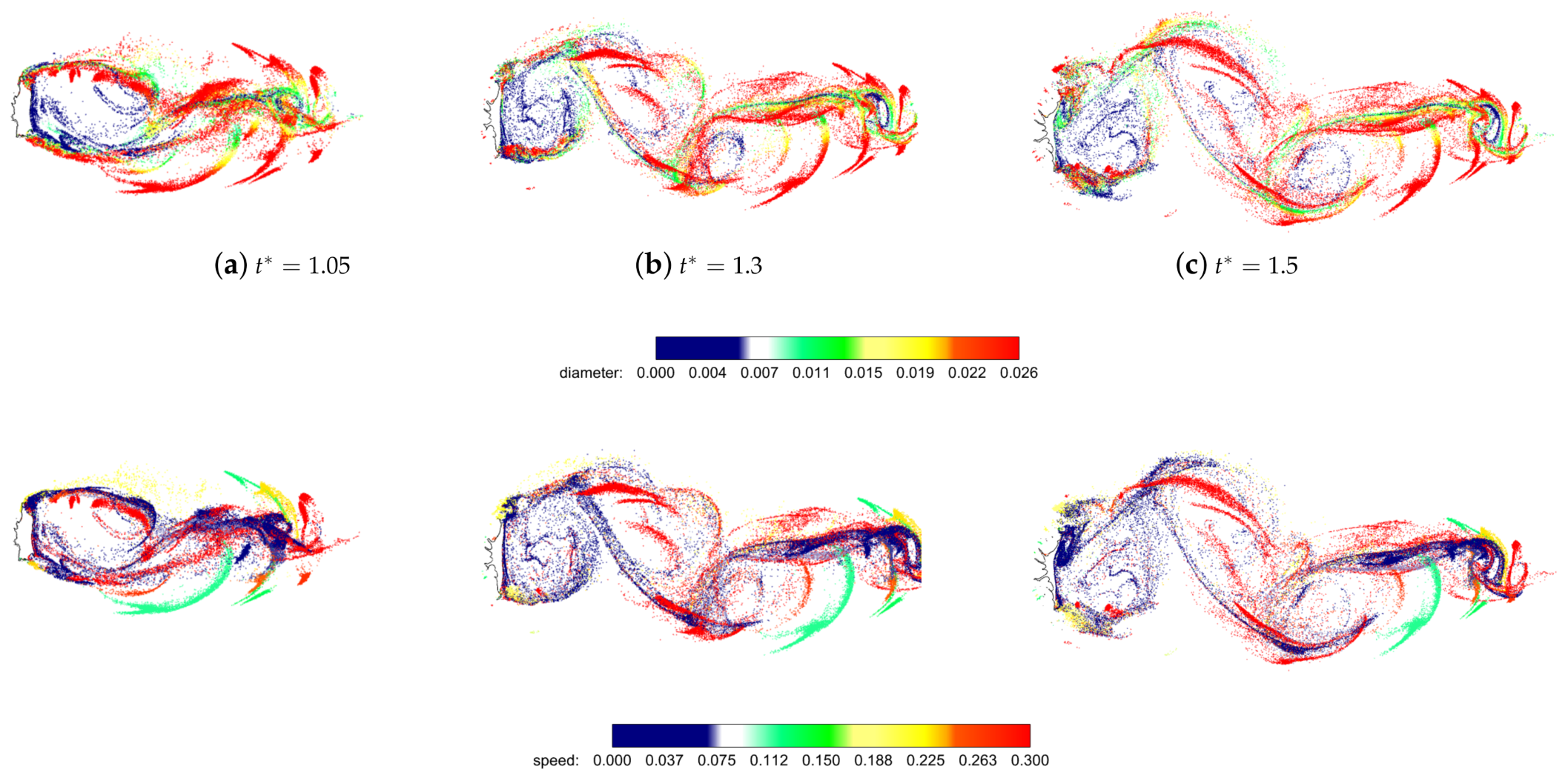
4.3. Sub-Droplets Tracking

A very important but less investigated aspect of droplet aerobreakup under the SIE regime concerns the dynamics of the dense mist of sub-droplets that is forming as a result of the droplet disintegration. In this study, due to the adoption of the hybrid VOF/DPM methodology, we can effectively simulate all stages of the shock-induced breakup, including the birth and the dynamics of small liquid particles that are consequently originated. Differently from what was recently performed in the Eulerian/Lagrangian model proposed in [42], here, the number of Lagrangian particles is not predetermined, but is increasing with time depending on the verification of the two transition criteria discussed in Section 2.2. The VOF-to-DPM method employs a dynamic mesh adaptation strategy, where the mesh resolution is automatically increased in the transition region between the two different phases, according to the volume fraction gradient field. This is exemplified in Figure 8, where the plane views of the FV mesh at four typical time instants are shown, in the midplane $y=0$, along with the corresponding contours of the volume fraction gradient magnitude, which is normalized by the reciprocal of the minimum mesh size. The coupling of adaptive meshing with the VOF method allows for capturing the gas–liquid interfaces with increased resolution, improving the numerical predictions for given computational resources.

The simulation of the discrete phase, through the solution of the momentum balance Equation (4) for each particle, allows determining the spatial-temporal evolution of the sub-droplets in the mean turbulent flow. To illustrate the results, in Figure 9, the instantaneous positions of the DPM particles are reported at three typical time instants, while being colored by either the nondimensional diameter $d_p/d_0$ (top) or the nondimensional speed $u_p/u_{\mathrm{g}}$ (bottom). Apparently, the sub-droplets evolve following the gas stream flow in the complex wake of the residual water body. By inspection of these pictures, there is a lack of correspondence between size and speed, as the space-time evolution of DPM particles results in being quite complicated.

The statistical distribution of sub-droplets is examined in Figure 10, where the histograms report the percentage of DPM particles in terms of either normalized diameter or speed, at two different time instants. Seemingly, the particle–size and particle–speed distributions appear poly-disperse and time-dependent. This is not surprising since the aerobreakup under the SIE regime is a continuous and multi-stage phenomenon [8]. Indeed, the small-scale sub-droplets are continuously formed and entrained during the whole process, while the fragmentation occurs not only from the parent body but also from sheets and ligaments, as well as from smaller child droplets. Moreover, finer particles achieve higher speeds faster. When looking at the particles arising from the shear-stripping of liquid ligaments, the size distribution should resemble a Gamma function distribution [43]. This is approximately observed on the left side of Figure 10, where the theoretical behavior seems to be somewhat approached with increasing time.

Converting the smallest liquid lumps resulting from the dissolution of the parent body into point masses that can be tracked using the DPM model, the hybrid modeling approach provides insight into the sub-droplets dynamics, allowing to bypass the limits of experimental studies, where the dense mist investigation is extremely difficult. This way, the proposed CFD model is very promising to be used in the fluids engineering research. For instance, these results could be of particular importance when predicting the rain erosion on supersonic aircraft [44].

5. Conclusions

This work contributed to testing a novel method for the industrial CFD prediction of the droplet aerobreakup process while providing an insight into the mist formation and development, which is of particular interest for engineering design. The aerodynamic breakup of a liquid droplet was numerically simulated adopting a physically consistent and computationally efficient multiscale approach for two-phase flows. In contrast to our previous study [19], a hybrid VOF–Lagrangian model was implemented allowing us to simulate the dynamics of the small liquid fragments. Moreover, the mean turbulent compressible flow was approximated following the SAS-URANS approach leading to the better prediction of unsteady turbulent structures. The breakup features observed in the experiments which are deformation, fragmentation, and dispersion of the produced mist were reproduced with acceptable accuracy by the hybrid method, without being computationally cumbersome. The effectiveness of the proposed method was demonstrated by making both qualitative and quantitative comparisons with reference solutions provided by experimental visualizations and high-fidelity numerical simulations. That highlighted the benefits of the proposed relatively simple CFD model, which is also able to predict the characteristics of the secondary droplets within the produced mist.

As to future perspectives, the possibility of applying more sophisticated models based on wavelet multiscale methods [45,46] is under study. Very recently, this innovative approach employing the adaptive wavelet collocation method to solve the energetic flow structures on dynamic grids has been further developed for supersonic flows [47,48,49], and novel wavelet-based adaptive URANS models [50,51] might be explored in the present context [28].

References

1. Menter, F.; Hüppe, A.; Matyushenko, A.; Kolmogorov, D. An overview of hybrid RANS–LES models developed for industrial CFD. Appl. Sci. 2021, 11, 2459. [Google Scholar] [CrossRef]
2. Theofanous, T.G. Aerobreakup of Newtonian and viscoelastic liquids. Annu. Rev. Fluid Mech. 2011, 43, 661–690. [Google Scholar] [CrossRef]
3. Villermaux, E. Fragmentation. Annu. Rev. Fluid Mech. 2007, 39, 419–446. [Google Scholar] [CrossRef]
4. Moylan, B.; Landrum, B.; Russell, G. Investigation of the physical phenomena associated with rain impacts on supersonic and hypersonic flight vehicles. Procedia Eng. 2013, 58, 223–231. [Google Scholar] [CrossRef]
5. Theofanous, T.G.; Li, G.J. On the physics of aerobreakup. Phys. Fluids 2008, 20, 052103. [Google Scholar] [CrossRef]
6. Poplavski, S.; Minakov, A.; Shebeleva, A.; Boiko, V. On the interaction of water droplet with a shock wave: Experiment and numerical simulation. Int. J. Multiph. Flow 2020, 127, 103273. [Google Scholar] [CrossRef]
7. Igra, D.; Takayama, K. Investigation of aerodynamic breakup of a cylindrical water droplet. At. Sprays 2001, 11, 167–185. [Google Scholar]
8. Theofanous, T.G.; Mitkin, V.V.; Ng, C.L.; Chang, C.H.; Deng, X.; Sushchikh, S. The physics of aerobreakup. II. Viscous liquids. Phys. Fluids 2012, 24, 022104. [Google Scholar] [CrossRef]
9. Wang, Z.; Hopfes, T.; Giglmaier, M.; Adams, N.A. Effect of Mach number on droplet aerobreakup in shear stripping regime. Exp. Fluids 2020, 61, 193. [Google Scholar] [CrossRef]
10. Chen, H. Two-dimensional simulation of stripping breakup of a water droplet. AIAA J. 2008, 46, 1135. [Google Scholar] [CrossRef]
11. Stefanitsis, D.; Koukouvinis, P.; Nikolopoulos, N.; Gavaises, M. Numerical investigation of the aerodynamic droplet breakup at Mach numbers greater than 1. J. Energy Eng. 2021, 147, 04020077. [Google Scholar] [CrossRef]
12. Zhu, W.; Zheng, H.; Zhao, N. Numerical investigations on the deformation and breakup of an n-decane droplet induced by a shock wave. Phys. Fluids 2022, 34, 063306. [Google Scholar] [CrossRef]
13. Sembian, S.; Liverts, M.; Tillmark, N.; Apazidis, N. Plane shock wave interaction with a cylindrical water column. Phys. Fluids 2016, 28, 056102. [Google Scholar] [CrossRef]
14. Rossano, V.; De Stefano, G. Computational evaluation of shock wave interaction with a cylindrical water column. Appl. Sci. 2021, 11, 4934. [Google Scholar] [CrossRef]
15. Meng, J.C.; Colonius, T. Numerical simulation of the aerobreakup of a water droplet. J. Fluid Mech. 2018, 835, 1108–1135. [Google Scholar] [CrossRef]
16. Liu, N.; Wang, Z.; Sun, M.; Wang, H.; Wang, B. Numerical simulation of liquid droplet breakup in supersonic flows. Acta Astronaut. 2018, 145, 116–130. [Google Scholar] [CrossRef]
17. Allaire, G.; Clerc, S.; Kokh, S. A five-equation model for the simulation of interfaces between compressible fluids. J. Comput. Phys. 2002, 181, 577–616. [Google Scholar] [CrossRef]
18. Hirt, C.W.; Nichols, B.D. Volume of fluid (VOF) method for the dynamics of free boundaries. J. Comput. Phys. 1981, 39, 201–225. [Google Scholar] [CrossRef]
19. Rossano, V.; Cittadini, A.; De Stefano, G. Computational evaluation of shock wave interaction with a liquid droplet. Appl. Sci. 2022, 12, 1349. [Google Scholar] [CrossRef]
20. Menter, F.R.; Egorov, Y. The scale-adaptive simulation method for unsteady turbulent flow predictions. Part 1: Theory and model description. Flow Turbul. Combust. 2010, 85, 113–138. [Google Scholar] [CrossRef]
21. De Stefano, G.; Natale, N.; Reina, G.P.; Piccolo, A. Computational evaluation of aerodynamic loading on retractable landing-gears. Aerospace 2020, 7, 68. [Google Scholar] [CrossRef]
22. Iannelli, P.; Denaro, F.M.; De Stefano, G. A deconvolution-based fourth-order finite volume method for incompressible flows on non-uniform grids. Int. J. Numer. Methods Fluids 2003, 43, 431–462. [Google Scholar] [CrossRef]
23. Roberts, J.; Wypych, P.; Hastie, D.; Liao, R. Analysis and validation of a CFD-DPM method for simulating dust suppression sprays. Part. Sci. Technol. 2022, 40, 415–426. [Google Scholar] [CrossRef]
24. Amatriain, A.; Urionabarrenetxea, E.; Avello, A.; Martín, J.M. Multiphase model to predict particle size distributions in close-coupled gas atomization. Int. J. Multiph. Flow 2022, 154, 104138. [Google Scholar] [CrossRef]
25. Lin, S.; Wang, Y.; Sun, L.; Abouei Mehrizi, A.; Jin, Y.; Chen, L. Experimental and numerical investigations on the spreading dynamics of impinging liquid droplets on diverse wettable surfaces. Int. J. Multiph. Flow 2022, 153, 104135. [Google Scholar] [CrossRef]
26. Scardovelli, R.; Zaleski, S. Direct numerical simulation of free-surface and interfacial flow. Annu. Rev. Fluid Mech. 1999, 31, 567–603. [Google Scholar] [CrossRef]
27. Brackbill, J.U.; Kothe, D.B.; Zemach, C. A continuum method for modeling surface tension. J. Comput. Phys. 1992, 100, 335–354. [Google Scholar] [CrossRef]
28. Hosseinzadeh-Nik, Z.; Aslani, M.; Owkes, M.; Regele, J.D. Numerical simulation of a shock wave impacting a droplet using the adaptive wavelet-collocation method. In Proceedings of the ILASS-Americas 28th Annual Conference on Liquid Atomization and Spray Systems, Dearborn, MI, USA, 15–18 May 2016. [Google Scholar]
29. Schütze, J.; Gupta, V.K.; Aguado, P.L.; Hutcheson, P.; Esch, T.; Braun, M. Increasing the predictive character of spray process simulation by multiphase model transitioning. In Proceedings of the ILASS-Europe 29th Annual Conference on Liquid Atomization and Spray Systems, Paris, France, 2–4 September 2019. [Google Scholar]
30. Chang, P.; Xu, G.; Huang, J. Numerical study on DPM dispersion and distribution in an underground development face based on dynamic mesh. Int. J. Min. Sci. Technol. 2020, 30, 471–475. [Google Scholar] [CrossRef]
31. Morsi, S.; Alexander, A. An investigation of particle trajectories in two-phase flow systems. J. Fluid Mech. 1972, 55, 193–208. [Google Scholar] [CrossRef]
32. Nykteri, G.; Gavaises, M. Droplet aerobreakup under the shear-induced entrainment regime using a multiscale two-fluid approach. Phys. Rev. Fluids 2021, 6, 084304. [Google Scholar] [CrossRef]
33. Shyue, K.M. A fluid-mixture type algorithm for barotropic two-fluid flow problems. J. Comput. Phys. 1998, 200, 718–748. [Google Scholar] [CrossRef]
34. Menter, F.R. Two-equation eddy-viscosity turbulence models for engineering applications. AIAA J. 1994, 32, 1598–1605. [Google Scholar] [CrossRef]
35. Egorov, Y.; Menter, F.R.; Lechner, R.; Cokljat, D. The scale-adaptive simulation method for unsteady flow predictions. Part 2: Application to complex flows. Flow Turbul. Combust. 2010, 85, 139–165. [Google Scholar] [CrossRef]
36. Menter, F.R.; Langtry, R.B.; Likki, S.R.; Suzen, Y.B.; Huang, P.G.; Völker, S. A correlation-based transition model using local variables - Part I: Model formulation. J. Turbomach. 2006, 128, 413–422. [Google Scholar] [CrossRef]
37. De Stefano, G.; Denaro, F.M.; Riccardi, G. High-order filtering for control volume flow simulation. Int. J. Numer. Methods Fluids 2001, 37, 797–835. [Google Scholar] [CrossRef]
38. Denaro, F.M.; De Stefano, G. A new development of the dynamic procedure in large-eddy simulation based on a finite volume integral approach. Application to stratified turbulence. Theoret. Comput. Fluid Dyn. 2011, 25, 315–355. [Google Scholar] [CrossRef]
39. Issa, R.I. Solution of the implicitly discretised fluid flow equations by operator-splitting. J. Comput. Phys. 1986, 62, 40–65. [Google Scholar] [CrossRef]
40. Leonard, B.P. A stable and accurate convective modelling procedure based on quadratic upstream interpolation. Comput. Methods Appl. Mech. Eng. 1979, 19, 59–98. [Google Scholar] [CrossRef]
41. Meng, J.C.; Colonius, T. Numerical simulations of the early stages of high-speed droplet breakup. Shock Waves 2015, 25, 399–414. [Google Scholar] [CrossRef]
42. Kaiser, J.W.J.; Appel, D.; Fritz, F.; Adami, S.; Adams, N.A. A multiresolution local-timestepping scheme for particle–laden multiphase flow simulations using a level-set and point-particle approach. Comput. Methods Appl. Mech. Eng. 2021, 384, 113966. [Google Scholar] [CrossRef]
43. Villermaux, E.; Marmottant, P.; Duplat, J. Ligament-mediated spray formation. Phys. Rev. Lett. 2004, 92, 074501. [Google Scholar] [CrossRef] [PubMed]
44. Gohardani, O. Impact of erosion testing aspects on current and future flight conditions. Prog. Aerosp. 2011, 47, 280–303. [Google Scholar] [CrossRef]
45. De Stefano, G.; Vasilyev, O.V. Hierarchical adaptive eddy-capturing approach for modeling and simulation of turbulent flows. Fluids 2021, 6, 83. [Google Scholar] [CrossRef]
46. Ge, X.; De Stefano, G.; Hussaini, M.Y.; Vasilyev, O.V. Wavelet-based adaptive eddy-resolving methods for modeling and simulation of complex wall-bounded compressible turbulent flows. Fluids 2021, 6, 331. [Google Scholar] [CrossRef]
47. De Stefano, G.; Brown-Dymkoski, E.; Vasilyev, O.V. Wavelet-based adaptive large-eddy simulation of supersonic channel flow. J. Fluid Mech. 2020, 901, A13. [Google Scholar] [CrossRef]
48. Kasimov, N.; Dymkoski, E.; De Stefano, G.; Vasilyev, O.V. Galilean-invariant characteristic-based volume penalization method for supersonic flows with moving boundaries. Fluids 2021, 6, 293. [Google Scholar] [CrossRef]
49. De Stefano, G.; Dymkoski, E.; Vasilyev, O.V. Localized dynamic kinetic-energy model for compressible wavelet-based adaptive large-eddy simulation. Phys. Rev. Fluids 2022, 7, 054604. [Google Scholar] [CrossRef]
50. Ge, X.; Vasilyev, O.V.; De Stefano, G.; Hussaini, M.Y. Wavelet-based adaptive unsteady Reynolds-averaged Navier-Stokes computations of wall-bounded internal and external compressible turbulent flows. In Proceedings of the 2018 AIAA Aerospace Sciences Meeting, Kissimmee, FL, USA, 8–12 January 2018. AIAA Paper 2018-0545. [Google Scholar]
51. Ge, X.; Vasilyev, O.V.; De Stefano, G.; Hussaini, M.Y. Wavelet-based adaptive unsteady Reynolds-averaged Navier-Stokes simulations of wall-bounded compressible turbulent flows. AIAA J. 2020, 58, 1529–1549. [Google Scholar] [CrossRef]
Figure 1. Normalized pressure contours depicted in the midplane y = 0 , as well as on the droplet boundary, at four typical time instants with 0.044 t * 0.25 . Both front (top) and back (bottom) views are shown.
Applsci 12 08302 g001
Figure 2. Normalized pressure contours depicted in the midplane y = 0 , as well as on the droplet boundary, at four typical time instants with 0.43 t * 0.83 . Both front (top) and back (bottom) views are shown.
Applsci 12 08302 g002
Figure 3. Normalized vorticity contours depicted in the midplane y = 0 , as well as on the droplet boundary, at eight typical time instants.
Applsci 12 08302 g003
Figure 4. Predicted droplet morphology (top) compared to experimental images by Theofanous and co-workers [8] (bottom), at six typical time instants. The airflow is from right to left.
Applsci 12 08302 g004
Figure 5. Contour plots for the normalized density of the gas phase depicted in the plane x / d 0 = 1 , at four typical time instants.
Applsci 12 08302 g005
Figure 6. Normalized displacement (left) and velocity (right) of the droplet CM for SAS-URANS, URANS [19], and DNS [15].
Applsci 12 08302 g006
Figure 7. Normalized acceleration of CM (left) and drag coefficient (right) of the droplet for SAS-URANS, URANS [19], and DNS [15].
Applsci 12 08302 g007
Figure 8. Plane views in the midplane y = 0 of adaptive numerical mesh (top) and corresponding contours of normalized volume fraction gradient magnitude (bottom) at four typical time instants.
Applsci 12 08302 g008
Figure 9. Plane views in the midplane y = 0 of instantaneous positions of DPM particles at three typical time instants, colored by either nondimensional diameter (top) or speed (bottom).
Applsci 12 08302 g009
Figure 10. Percentage distributions of DPM particle sizes (left) and particle speeds (right) at two different time instants that are t * = 1.75 (red and blue) and t * = 2 (cyan and green).
Applsci 12 08302 g010