Data Augmentation in 2D Feature Space for Intelligent Weak Fault Diagnosis of Planetary Gearbox Bearing

Featured Application

Planetary gearbox bearings weak faults Intelligent diagnosis.

Abstract

Quickly detecting and accurately diagnosing early bearing faults is the key to ensuring the stable operation of high-precision equipment. In actual industrial applications, it is common to face the issues of big data and poor fault identification accuracy. To accurately and automatically realize the diagnostics of rolling bearings, a convolutional neural network algorithm and fault feature enhancement method is proposed. A two-dimensional space feature extraction method based on the Cyclostationary theory and wavelet transform shows good results in noise suppression. Firstly, the cyclic demodulation of wavelet transform coefficients is performed on bearing vibration signals to convert one-dimensional vibration data into a two-dimensional spectrogram for enhancing the weak fault feature. Secondly, the image segmentation theory is introduced, which can obtain more data and improve the calculation accuracy and efficiency on the basis of data dimension reduction. Finally, the augmented 2D spectrograms are inputted into a convolutional neural network. Through the analysis of the actual planetary gearbox bearing data, and compared with other mainstream intelligence algorithms, the effectiveness and superiority of this method are verified.

1. Introduction

The planetary gearbox is widely used in wind turbines, modern vehicles, ships and warships, helicopters, and many other applications. As such gearboxes are fundamental for power transfer, they are often mission critical and safety critical, so ensuring stable and safe operation is vitally important for their production and life. As a crucial component of the gearbox, the planetary bearing is more subject to the external environment, coupling between structures, loads, and working conditions than other structural components. Thus, the vibration signal patterns related to the bearings are more complicated, which makes its health monitoring and diagnostics more difficult. Early damage detection is a key diagnostics requirement for ensuring safe high-precision equipment operation, eventually enabling predictive maintenance. However, the features that characterize early damage are relatively weak and hidden by large external interference. In addition, big amounts of data will be generated during industrial operation, so a great challenge is to propose novel diagnostics tools to substitute the traditional signal processing-based methods which may be impractical for the planetary gearbox bearing fault diagnostics. In fact, there is an urgent need for a high-efficiency and high-precision algorithm for batch data processing robust to external interference.

Artificial neural networks [1], support vector machines [2], and deep learning [3] are three of the most representative intelligent fault diagnosis methods which were used by many scholars to realize batch processing of vibration data. It is found that the traditional neural network algorithm underperformed in terms of structural robustness, adaptability, and accuracy for weak signals. A support Vector Machine (SVM) is limited in processing high-dimensional multi-class data. The deep learning method has become a popular algorithm with its excellent performance, which has won the favor of researchers.

The greatest advantage of deep learning is that there is no need to manually select features during operation. Deep learning algorithms automatically learn how to extract the target information of the original data layer by layer through multiple nonlinear connection layers enabling the extraction of complex features. The existing deep learning network structures include: the Convolutional Deep Neural Network (CNN) [4,5,6], Deep Belief Network (DBN) [7], Recurrent Neural Network (RNN) [8], Sparse Autoencoder (SAE) [9], etc. It is widely applied in image processing and pattern recognition.

Among the deep learning algorithms, CNN was the first deep learning network structure to be proposed. It has attracted the attention of researchers in many fields and has achieved remarkable results, such as bearing fault diagnosis. Fu et al. [10] proposed a new convolution theory based on feature fusion which can improve the adaptive ability of the algorithm in different feature scale-spaces. Wang et al. [11] proposed a method to optimize the parameters of the deep CNN model using a particle group algorithm, which can remove the influence of prior knowledge on fault diagnosis results. Jia et al. [12] normalized the data and gave different weights to the loss function with different distribution ratios to weaken the class shift of the sample recognition results in the case of data imbalance. Wang et al. [13] applied a multi-head attention to optimize the CNN structure, which improved the accuracy of identification. Although these methods led to good diagnostics results, issues related to poor diagnostic performance for weak fault signals with low signal-to-noise ratios and small relative amplitudes remain unresolved.

The fault diagnosis method based on deep learning requires massive learning datasets to accurately reveal the internal structure and characteristic behavior of the analyzed signals. However, direct analysis of the observed weak fault signals will inevitably underperform, as the raw signals contain a large amount of noise and strong contributions from rotating shafts and gears unrelated to bearing faults. Therefore, to improve the accuracy of the diagnostics, it is key to use an appropriate algorithm for fault characteristic signal enhancement so as to highlight the relevant information. For example, Islam [14] proposed wavelet packet transform as a 2D visualization tool and applied CNN to recognize bearing conditions. Wavelet packet transform time-frequency feature fusion is also an effective method for enhancing fault characteristics [15]. The sub-components of the decomposed signal can be input to CNN for extracting more fault-sensitive information to improve the results of the degradation assessment. Xu et al. [16] used Variational Mode Decomposition (VMD) as a preprocessing algorithm to decompose the original signal into Intrinsic Mode Functions (IMFs), and then input them into the CNN network to extract the characteristics of each IMF. The validity of the algorithm is verified by experiment data under different environments and operating states. Shao et al. [17] proposed multi-sensor information fusion technology, which can provide more accurate information for weak fault classification. However, most of the condition monitoring data collected in the actual service environment are non-faulty state data, and the amount of vibration data in the faulty state is relatively small. Even if the vibration data in the fault state are collected, the unique structure of planetary bearings leads to complex peculiar vibration patterns which are not easily highlightable.

The attenuation characteristic of the signal transmission path is the main factor leading to the weak fault characteristic of the planetary bearing measuring point signal. The operating environment of mechanical equipment is harsh, and the external interference is large. Early fault patterns are often flooded by external information unrelated to the fault. In addition, the coupled movement between the different planetary gearbox parts leads to complex non-stationary, modulated signals due to variable transmission paths and variable loads. Finally, a certain fault characteristic may be covered by other fault characteristics, resulting in multiple fault signal characteristics cross coverage, which is another critical characteristic of fault characteristic signals.

Taking into account the above factors, it has been found that Cyclostationary analysis can be applied to the non-stationary fault signal analysis of planetary bearings. In fact, even if the time-domain fault-characteristic waveform is not cyclical, its statistics generally change with time and show period or multi-period changes [18]. Cyclostationary analysis tools such as the spectral correlation density [19,20], cyclic modulation spectrum [21], FFT cumulative method [22], cycle energy indicators [23], and the rapid spectral estimation algorithm [24,25] have been proven to be effective in the field of weak fault diagnostics. In order to improve the recognition accuracy of the CNN algorithm, in the preprocessing step, wavelet transform coefficients cyclic demodulation (WSC) is proposed to obtain a 2D spectrometography able to enhance the planetary gearbox bearing fault characteristics.

In order to properly test the here proposed algorithm, a high-quality, labeled training dataset was used, containing acquisitions from a damaged condition. The novel proposed algorithm is described in Section 3, based on the notions about Cyclostationary (Section 2.1) and CNN (Section 2.2). WSC is adopted to eliminate the fault irrelevant information, isolate the fault source, and extract the fault-related feature quantity. Then, a 2D feature space data argumentation strategy based on image segmentation is proposed to compensate for the influence of the wavelet scale analysis range on the results. Afterward, the fault classification problem is realized by constructing a CNN analysis model and setting the parameters of each layer. Finally, the damage detection effectiveness of the proposed algorithm is assessed in Section 4.

2. Theoretical Background

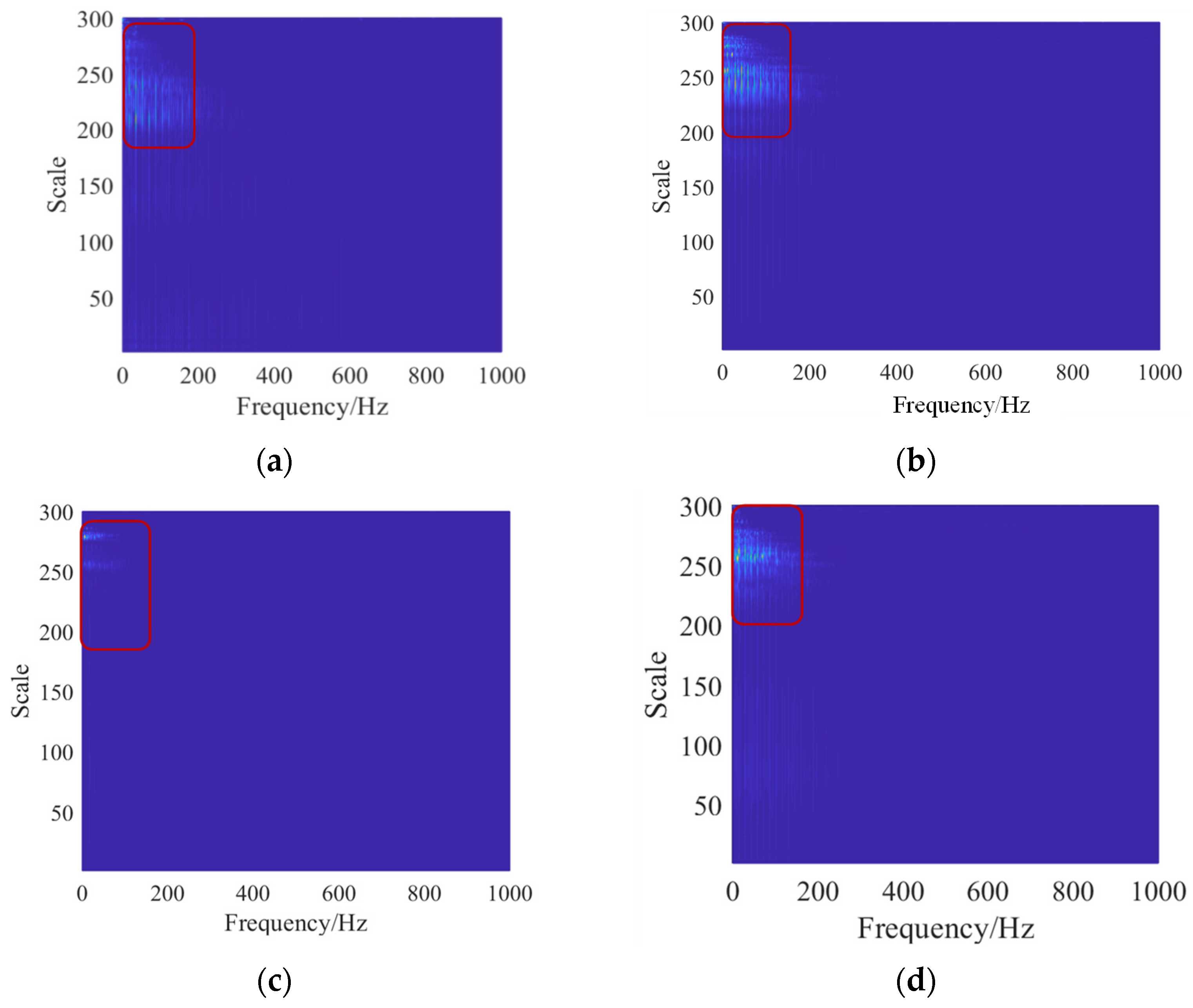
2.1. Cyclostationary Spectrometography

Rotating machinery equipment will produce periodic transient information in the event of a failure. Even if this information presents characteristics such as small amplitude, low energy, or high noise, it is a useful component for health diagnosis. The focus is on how to extract these characteristics from the measured signal. According to the Cyclostationary theory, the characteristic of interest can be obtained by calculating its statistics. Suppose $x(n)(n=1,2,3\dots N)$ is the original signal to be processed. N is the size of x. The following expressions show the characteristic of a Cyclostationary signal [18]:

$$C_{1x}(t)=\mathrm{E}\left\{x(t)\right\}=C_{1x}(t+T)$$

(1)

where $\mathrm{E}$ is the averaging operator and t is time. C_1x is the first-order cyclic statistics, which is periodic, and T is the Period of C_1x. It is obtained by averaging the first-order cycle smooth signal, as described in Equation (1). After the non-stationary signal x is processed by Equation (1), it can be transformed into a periodic signal with period T. A similar result can be obtained on a second-order cyclostationary signal. Given a time offset $\tau$, Equation (2) introduces second-order cyclic statistics [18]:

$$C_{2x}(t,\tau )=\mathrm{E}\left\{x(t)x^{\ast }(t-\tau )\right\}=C_{2x}(t+\tau ,T)$$

(2)

where C_2x is the second-order cyclic statistic and x* is the conjugate of x.

In addition to the two conversion methods shown in Equations (1) and (2), there are also multi-order cyclostationary analysis methods, which can reveal more complex periodic information hidden in the signal. Since the cyclic statistical quantity in the signal can present periodic components, a Fourier transform can be used to directly reflect its distribution regularity with frequency value, leading to the so-called cyclic autocorrelation function spectrum, as described in Equation (3) [19].

$$S_x^{}(f)=\frac{1}{T}{\displaystyle {\int }_{-\infty }^{\infty }{\displaystyle \sum _{n=-N}^N\underset{N\to \infty }{\lim }}\frac{1}{2N+1}{\displaystyle {\int }_{-\frac{T}{2}}^{\frac{T}{2}}x(t+n{T}_{})}}{x}^{\ast }(t+n{T}_{}-\tau )e^{-i2\pi ft}{e}^{-i2\pi f\tau }dtd\tau$$

(3)

wherein, S_x(f) is cyclic autocorrelation function spectrum, the calculated f is also called cyclic frequency.

According to analysis, most of the bearing vibration signals observed under fault conditions will cause some form of cyclostationary characteristics. However, the cyclostationary method based on the first-order and second-order statistics is less robust and the effect is not good for the early weak fault diagnosis. In view of this problem, some researchers put forward the calculation of the periodic spectrum. The principle is to transform the signal by two Fourier transforms, applying Fourier transform coefficients instead of statistics to acquire a cyclic spectrum. It can be expressed as Equations (4) and (5):

$$C_{L,N,P}^{(h)}[m,k,f]=\frac{{\Delta }_t}{{\Vert h(n{\Delta }_t)\Vert }^2}{\displaystyle \sum _{n=0}^{N-1}(h[n]x[k,n+mP])e^{-2\pi j\frac{fn}{N}}}$$

(4)

$$CM{S}_x[k,f]=\frac{2}{M{\Delta }_t}{\displaystyle \sum _{m=0}^{M-1}{C}_{L,N,P}^{(h)}[m,k,f]e^{-2\pi j\frac{kfP}{N}}}$$

(5)

wherein, $h\left[n\right]$ is window function;${\Delta }_t$ is the sampling period; $L$ is the size of $h\left[n\right]$; f is spectral frequency points, and $f=0,\cdots ,\frac{L}{2}-1$; M is the number of sub-segment window function scanned; m is cyclic frequency points, and $m=0,\cdots ,\frac{M}{2}-1$; the overlap length of h$\left[n\right]$ is N-P; it can be seen from Equations (4) and (5) that the whole calculation process of the periodic spectrum can be regarded as a down-sampling process. At the same time, the accuracy of the results is affected by the type and size of $h\left[n\right]$. It can only extract valid period information, which is not a good match for the impact component.

2.2. Fault Classification Model

CNN is the first proposed deep learning model, which is highly applied in image processing, voice translation, state classification, and other fields. The CNN model realizes sample identification and classification by sensing the information in the local range of samples and realizing the information interaction between network layers through parameter sharing. In general, the CNN model mainly consists of an input layer, convolution layer, pooling layer, full connection layer, and output layer, including a softmax activation function. Among them, the input layer is mainly to preprocess the raw data and images of the input. The functions and structures of the other layers are as follows:

2.2.1. Convolution Layer

The convolutional layer is meant to extract the features of the input samples, and it also has the effect of dimensionality reduction.

2.2.2. Pooling Layer

The pooling layer is a feature enhancement layer based on the down-sampling principle. It is mainly achieved by modularizing the feature mapping image and calculation of its average or maximum value.

2.2.3. Fully Connected Layer

The fully connected layer first integrates multi-dimensional data into one-dimensional data. There may be more than one fully connected layer, and the layers are usually connected by weights, as shown in Figure 1.

Assume that the neurons of the one-dimensional input layer after high-dimensional data integration are p₁, p₂, and p₃. The nodes in the middle layer are $a_i^{\left(l\right)}$, which represents the activation values of the i-th neuron in layer l. $w_{i,j}^{\left(l\right)}$ represents the weight values of the connection parameter between the j-th neuron of layer L and the i-th neuron of the next layer. $b_i^{\left(l\right)}$ is bias item of the i neuron of layer l. It can be seen from Figure 1 that the output of layer L neurons is the input of layer L + 1 neurons. According to Figure 1, the following expression can be obtained:

$$a_i^l={\displaystyle \sum _{j=1}^n{w}_{i,j}^{(l-1)}{a}_j^{l-1}}+b_j^{l-1}$$

(6)

The above process is also called the coding process, which reflects the internal characteristic information of the original signal. The last hidden layer outputs the most advanced features of the input signal. The classification result of the whole network is related to the selection of parameters in the model. In order to further improve the robustness of the model, the feature quantity with large inter-layer correlation is extracted as the subsequent processing object to eliminate the influence of interference factors on the results, as shown in Equation (7).

$$a_i^l=\{\begin{array}{cc}0& a_i^l\le 0\\ a_i^l& a_i^l>0\end{array}$$

(7)

2.2.4. Output Layer

In order to realize the classification of input samples, an activation function is usually set after the full connection layer. Suppose the input is x, and the probability of predicting that its category belongs to y is P. The sum of the probabilities that x belongs to all possible types is 1. The type corresponding to the maximum probability value is selected as the output of the network. The expression is:

$$P(x=y_i)=\frac{e^{a_i^{\left(l\right)}}}{{\displaystyle \sum _{i=1}^S{e}^{{}^{a_i^{\left(l\right)}}}}}$$

(8)

where S is the number of categories and $a_i^{\left(l\right)}$ is the output of layer l, that is, the input node of the softmax layer.

3. The Proposed Method

3.1. Construction of Two-Dimensional Feature Space

The fault signal of the rolling bearing presents cyclostationary characteristics, so the fault source information can be highlighted by extracting its cyclostationary quantity. Therefore, based on the idea of the cyclic spectrum, this paper constructs a two-dimensional feature space to realize the feature enhancement of weak signals. As mentioned in Section 2.1, the calculation efficiency of high-order cyclostationary quantities is low, and the cyclic periodic spectrum is affected by the window function, which is not suitable for the pre-processing process of model data. However, compared with the Fourier transform, the wavelet function has stronger adaptability in some cases and performs well in fault diagnosis. To improve adaptability, wavelet transformation coefficients are proposed to replace the Fourier transform coefficients. As described in Equation (9):

$$\begin{array}{ll}W{T}_x(a,b)& =\frac{1}{\sqrt{a}}{\displaystyle {\int }_{-\infty }^{\infty }{\displaystyle {\int }_{-\infty }^{\infty }x(t){\Psi }^{\ast }}}(\frac{t-b}{a})e^{-j2\pi ft}dadt\\ & ={\displaystyle {\int }_{-\infty }^{\infty }\langle x(t),{\Psi }_{a,b}(t)\rangle e^{-j2\pi ft}dt}\end{array}$$

(9)

where ${\Psi }^{}$ is the waveform basis function; ${\Psi }^{\ast }$ is the conjugate of ${\Psi }^{}$; ${\Psi }_{a,b}(t)$ is obtained by performing time direction translation and scale direction scaling on the basic wavelet function; a is the scale factor; and b is the time factor.

Through the study of the fault mechanism of rolling bearings, as described in paper [26], the fault signal characteristics of rolling bearings are close to the Morlet wavelet. Therefore, Morlet is used as a wavelet basis for analysis when constructing two-dimensional feature space based on WSC.

3.2. Data Augmentation Based on WSC Image Segmentation

Planetary gearboxes are designed for large loading capacity, high transmission efficiency, strong shock resistance, and vibration resistance. It is also because of its unique performance that its operating environment is worse and the collected vibration signal is more complex. The transmission path of the fault excitation signal, the contact force between components, and the attenuation characteristics caused by load fluctuations will add modulation components to the vibration signal of the planetary bearing. In addition, the planetary gearbox bearing fault signal often contains complex noise components due to the harsh operating environment of mechanical equipment and large external interference. In this case, traditional time-frequency analysis methods fail to reveal fault-related feature information. Most of the planetary bearings’ vibration signals in the fault state will cause some form of Cyclostationarity, which leads to the discrete peak of the envelope spectrum in the fault characteristic frequency.

In this paper, aiming at the problems existing in the research of current fault diagnosis theory and methods, considering the characteristics of the vibration signal collected under actual working conditions, such as small amplitude, low energy, and large noise, the purpose is to explore the fault source information enhancement mechanism of label data based on a CNN deep classification network. In order to further optimize the weight coefficient, a parameter self-adjusting (PSA) method based on multiple error back propagation is applied in this paper.

It is undoubtedly more representative data that can improve the classification effect of the model. However, it is difficult to meet this requirement in practical application. Small disturbances will bring bias to the diagnostic results based on the data-driven model, which requires the analysis samples to be representative and have relatively clear target characteristics. In this paper, a mechanism for enhancing fault source information based on the cyclic wavelet spectrum is proposed, aiming at the characteristics of the small amplitude, low energy, and strong noise of the planetary bearing vibration signal. The wavelet transform coefficients are regarded as a special cyclic statistic to calculate the cyclic spectrum so that the non-stationary fault-characteristic signal of the planetary gearbox bearing is transformed into a periodic stationary signal, which can reduce the interference of irrelevant information and enhance the impact characteristics. However, it will increase the computational burden of the algorithm. In order to improve the computational efficiency of the algorithm, this paper proposes to further segment the cyclic spectrum to use local features of samples as the matching object. On the one hand, it can reduce the size of a single sample; on the other hand, it can enhance the number of samples.

Image local feature extraction is realized by overlapping and blocking the image. When dividing the spectrum into blocks, a local overlapping is performed. Suppose the length of the overlapping area is q, it defines the small block as a square with an edge length of s. The visualized graphics are shown in Figure 2.

3.3. Model Operation Process

Assuming that the input image is a multi-dimensional matrix X, the size is I × J and the number of convolution kernels is C. The convolution operation process is expressed by the formula as:

$$B(c_1,c_2)={\displaystyle {\int }_{i=1}^I{\displaystyle {\int }_{\mathrm{j}=1}^{J}K}\ast X(i-c_1{r}_1,j-c_2{r}_1)}didj$$

(10)

where $K$ is the convolution kernel; $B$ is the output feature map; $r_1$ is the size of sliding convolution window; $\ast$ denotes the convolution operation.

For an input feature map image $B(c_1,c_2)$, calculating its average value and the output feature map P($u_1,u_2$) is obtained:

$$P(u_1,u_2)={\displaystyle {\int }_{c_1=1}^C{\displaystyle {\int }_{c_2=1}^C\frac{1}{r_2\times r_2}B(c_1+(u_1-1)\times r_2,c_2+(u_2-1)\times r_2)d}}{c}_{1}d{c}_2$$

(11)

where $r_2$ is the size of filter and the step length of each movement. The operation process of other parts of the model shall refer to the relevant explanation in Section 2.2.

3.4. Fault Diagnosis Based on WSC-CNNs

According to the analysis in Section 2 and Section 3, the procedure of the proposed method WSC-CNNs is described as follows:

Step 1: Set the wavelet scale analysis range, perform WSC analysis on the original acceleration data, and transform the one-dimensional time domain signal into a two-dimensional feature space map.

Step 2: Divide the WSC into several sub-areas, and each sub-area is used as the training sample set of the CNN model.

Step 3: According to the optimal classification results, select the appropriate number of iteration updates and learning factors. The parameters of each layer are shown in

Table 1. Parameters set of each layer.

Layer	Operation	Number of Filters	Filter Size	Activation Function	Output Size
Input	/	/	/	/	(100, 100)
Conv	Kernels	20	3 × 3	ReLu	(98, 98, 20)
Pooling	Pooling size	/	2 × 2	Ave	(49, 49, 20)
Conv	Kernels	20	2 × 2	ReLu	(48, 48, 20)
Pooling	Pooling size	/	2 × 2	Ave	(24, 24, 20)
FC	/	120	/	ReLu	(120, 1)
FC	/	C	/	Softmax	(C, 1)

.

Step 4: The algorithm proposed in this paper is performed to analyze the experimental data. Additionally, it is then used to obtain the classification results and the visualized spatial distribution map. The use of other algorithms as a comparison to analyze the data to verify the superiority of the algorithm is proposed in this paper.

The overall flowchart of the algorithm is shown in Figure 3.

4. Experimental Validation

4.1. Experimental Setup and Data Description

The experimental data were acquired on the test bench in Figure 4, which features a two-stage planetary gearbox. In addition, a parallel shaft gearbox supported by bearings, a variable speed drive motor, and a magnetic powder brake can be found. The driving power of the whole experimental bench is provided by a variable speed motor, and its maximum speed can reach 5000 rpm. Then, the torque output by the motor is connected to the input shaft of the first-stage planetary gearbox through the torque sensor and the encoder. The components are connected to each other so that the whole system can work smoothly. At the end of the test, the programmable magnetic brake provides resistance to the system and gradually stops the entire system.

In order to verify the ability of the proposed method to identify data from different health conditions, vibration signals of the first-stage planetary gearbox were collected under four conditions: normal condition, planetary gearbox bearing outer-race fault, planetary gearbox bearing inner-race fault, and planetary gearbox bearing roller fault. The acquisitions were performed at a sampling frequency of 15,360 Hz and a motor speed of 2100 rpm.

4.2. Analysis of Wavelet Cyclic Spectrum

The most effective standard for distinguishing fault signals induced by different positions on the same equipment is the characteristic frequency components generated by the rolling elements passing the fault position in each fault condition. For early fault signals or weak fault signals with large external interference, the fault characteristic frequency is often overwhelmed by the rotation frequency or noise components. In order to strengthen the target information representation and expression ability of each signal in the data set, this paper proposed a pre-processing method of wavelet cycle frequency feature extraction to enhance the fault feature frequency. The wavelet cycle spectrums for different conditions are shown in Figure 5. It can be observed that fault-related information is mainly concentrated in the low frequency region. In order to clearly illustrate the target information enhancement ability of the proposed algorithm, the low frequency region spectrum is amplified locally, shown in Figure 6. In Figure 6a, there are only rotation frequency and harmonic components of the planet carrier and sun gear, corresponding to the normal condition. In Figure 6b–d, the components related to the fault of the inner race outer race and rolling elements of the planetary bearing are highlighted.

It can be concluded that the wavelet cycle spectrum is very effective in enhancing fault characteristic information. The cyclic characteristic information spectrum is input into a CNN model as an analysis data set, which can eliminate the interference of irrelevant information to a certain extent and improve the representation ability of the model for target information.

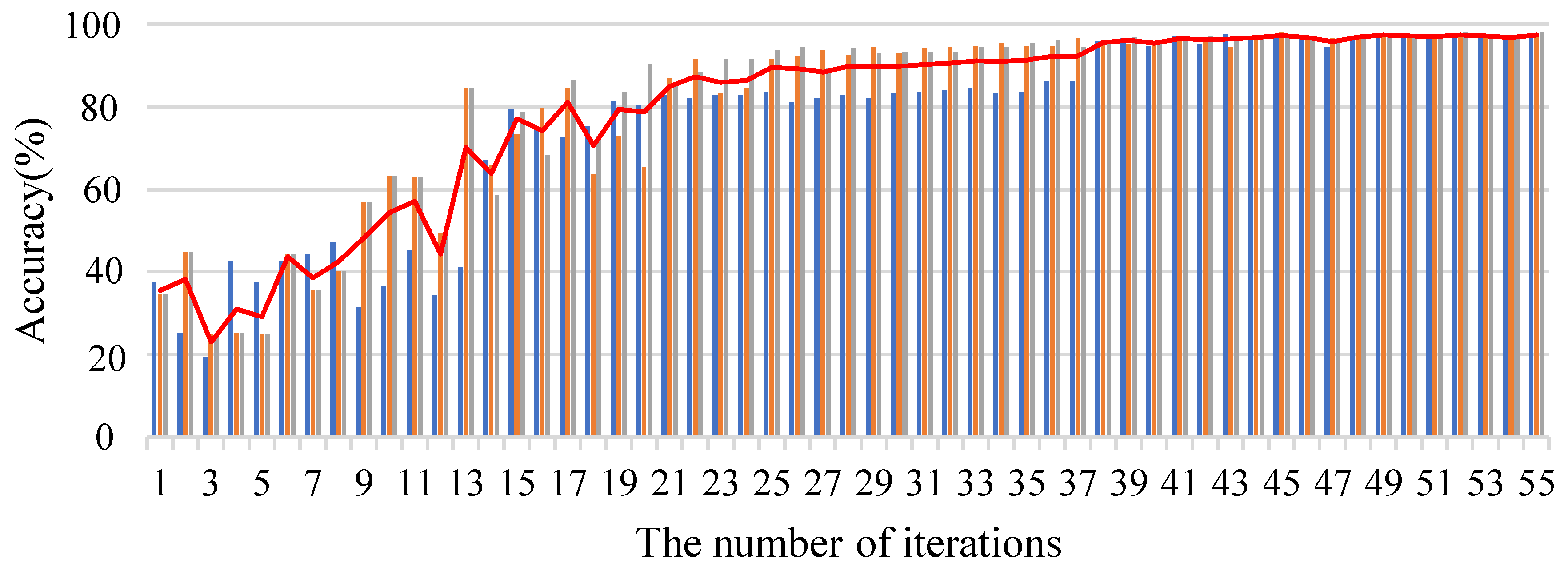
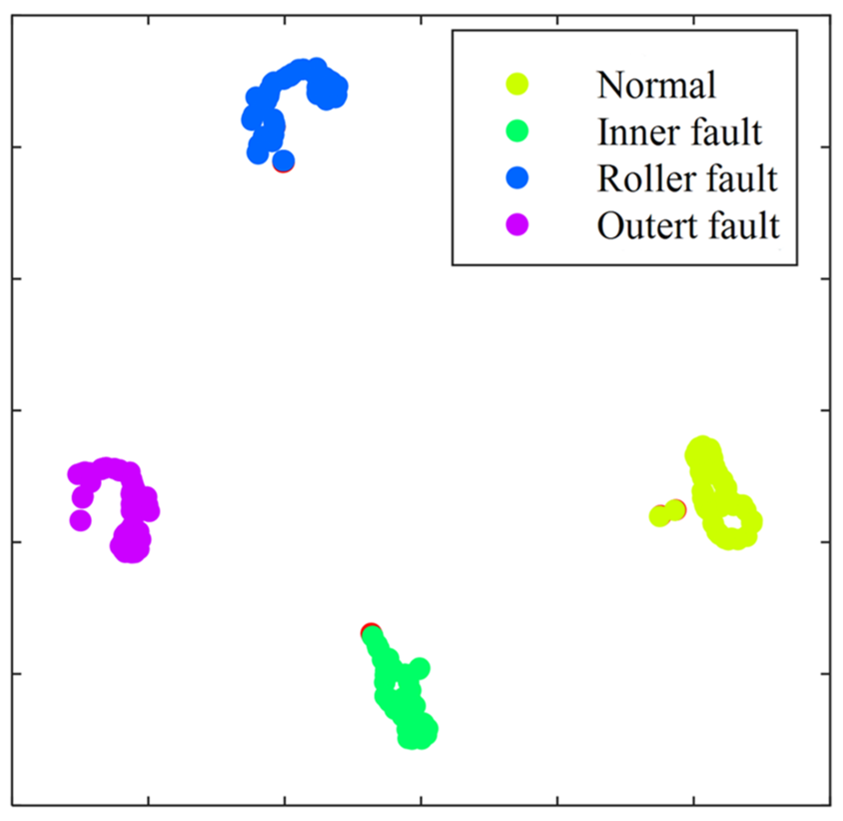
4.3. Fault Diagnosis Based on Data Feature Argumentation and CNN Model

In order to further verify the fault diagnosis effect of the proposed algorithm, the time domain signal is first collected for analysis. In total, 400 groups of data under each condition were collected as the training sample set, and then cyclic spectrum analysis was performed on it. At the same time, each set of conditions collected 70 sets of data as a test data set, shown as

Table 2. Test condition description.

Fault Type Number	Fault Location	Training Sample Size	Testing Sample Size
1	Normal	400	70
2	Inner-race Fault	400	70
3	Outer-race Fault	400	70
4	Ball Fault	400	70

. Subsequently, test data set is input into the model for analysis.

During the analysis, the model parameters are first determined. The Gaussian kernel function is used to initialize the convolutional layer connection coefficients. During the weight update phase, the learning rate $\eta$ and weight update coefficient $\beta$ have a great influence on the identification results. Based on the experience accumulated in the previous research process, to prevent overfitting, set $\eta$ and $\beta$ to 0.001 and 0.95, respectively. In addition, the weight update times are studied; increase the number of update times of connection weights and calculate the recognition accuracy rate corresponding to each update number. Perform three times continuously and the results are shown in the histogram of the three colors in Figure 7. Among them, the red curve represents the average recognition accuracy. It can be seen from the figure, by increasing the number of iterations, the matching degree of the system and the stability of the results can be improved, but it will bring a computational disaster. To balance the calculation efficiency and classification results, the number of weight updates is set to 49. Using the algorithm proposed in this paper, the final classification accuracy is 97.86%.

To further improve the visualization of classification results, the spatial representation feature analysis diagram obtained by t-SNE is shown in Figure 8. It displayed that the planetary bearing condition monitoring data after two-dimensional spatial feature extraction can enhance intra-class aggregation and class-to-class differentiation.

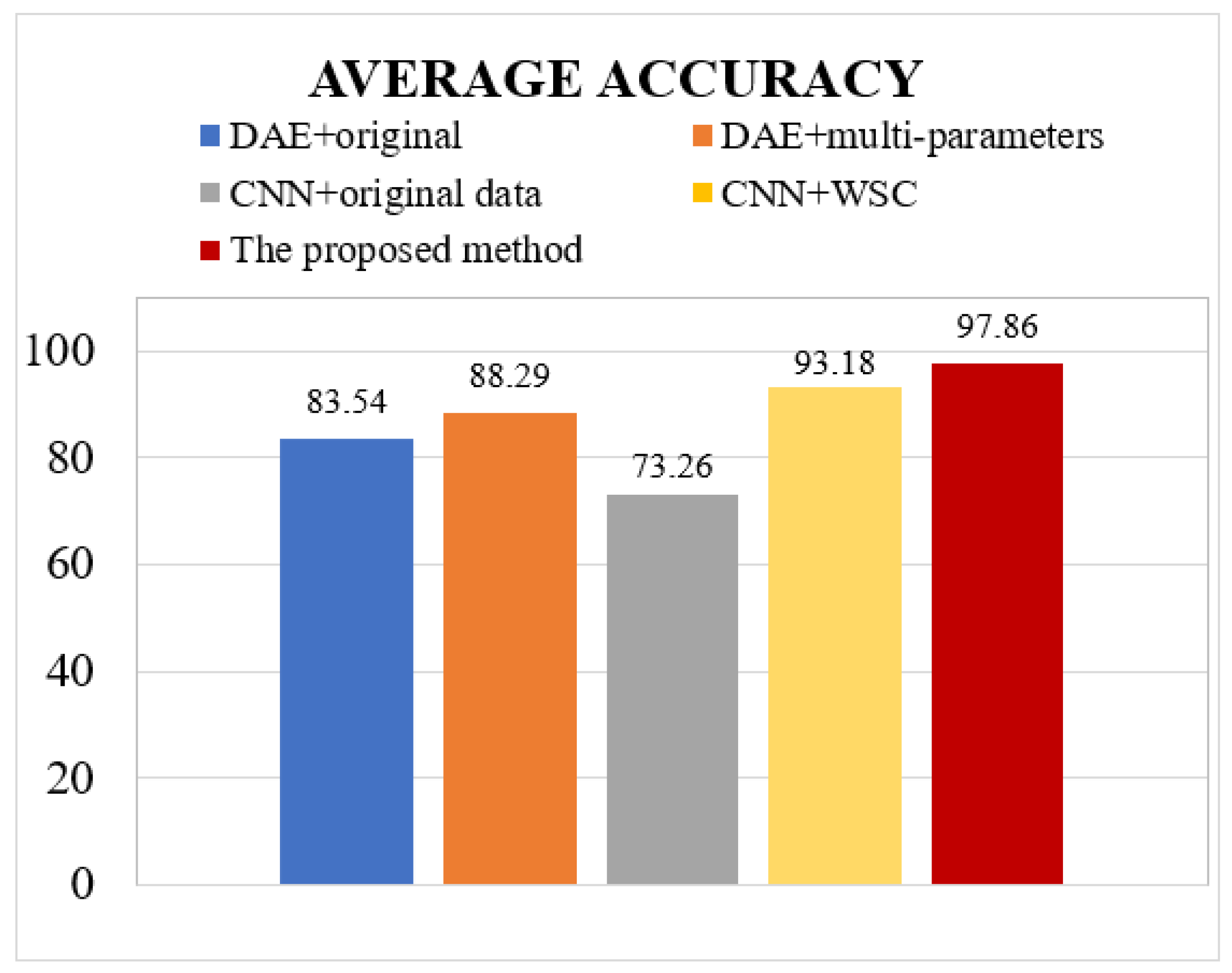
4.4. Comparison with Other Methods

To further verify the effectiveness of the methods proposed in this paper, other benchmark algorithms are used as a reference for comparison. Including the results of analyzing the original data and multi-parameter (mean value, root mean square value, variance, kurtosis value, minimum value, maximum value, and peak-to-peak value) sample set by using the DAE algorithm. It also includes results obtained by inputting raw data as well as un-enhanced, WSC pre-processed 2D images into the CNN model. The results are shown in Figure 9. The original time-domain data are directly inputted into the deep autoencoding model, and the classification accuracy rate is about 83.54%. Further extract multiple feature parameters of the time domain signal and input them into the deep auto-encoding model; although the classification accuracy has been improved, the average accuracy of the multiple classification results is only 88.29%. If the time domain signal is directly input to the one-dimensional CNN model, only 71% of the recognition accuracy can be obtained. Applying the method proposed in this paper, the one-dimensional time-domain signal is converted into two-dimensional data by calculating the WSC and then inputted into the two-dimensional CNN model for analysis, which can accurately identify 93.18% of the fault types. Further using the method of image segmentation to augment the data can improve the recognition accuracy to 97.86%.

Use t-SNE to visualize the characteristic manifolds obtained by the one-dimensional CNN model, as shown in Figure 10. The monitored vibration data under the healthy condition can be gathered together well, and it is more distinguishable from other fault types. Compared with Figure 8, the other three types of fault data have relatively small intra-class aggregation and inter-class differences. This is attributable to the fact that in the case of large external interference, the early fault features are weak and easy to be overwhelmed by random noise components, which affects the matching of target information. After the pre-processing of the feature enhancement, the characteristic information related to the fault is clarified. The difference of different fault feature information is used to improve the recognition ability of the model for different types of faults.

5. Conclusions

Planetary gearbox bearings diagnostics is not an easy task. In most of the industrial applications, in fact, the data quality is low, as it is very likely to find large amount of external noise, strong rotation frequency, and other information irrelevant to the fault in the training data. In these cases, traditional diagnostic tools cannot give a high-confidence output, and the recognition accuracy will be low. To solve this problem, a novel WSC-CNNs model with data argumentation in enhanced 2D feature space is established to address the weak fault diagnosis of planetary bearings. WSC is used as for pre-processing to extract the characteristic information of one-dimensional data, expanding it to a two-dimensional time-frequency map. Different fault types will show different spatial distribution characteristics in WSC, which increases the distance between healthy and damaged features. Subsequently, a 2D feature space data argumentation strategy based on image segmentation is proposed, and the fault feature concentration area is divided into sub-regions, which can improve the efficiency of the algorithm and enrich the sample set. Additionally, then, the augmented 2D WSC image is fed into a CNN, which can be very efficient for planetary bearing classification. Compared with other traditional benchmark algorithms, the proposed algorithm can improve the recognition ability of the weak fault signal of the planetary bearing. Compared with the DAE algorithm, the recognition accuracy of the proposed algorithm is improved by 9.57%. Compared with the direct analysis of the original data by the CNN model, the accuracy rate obtained by using WSC pre-processing as the sample set is increased by 19.92%. Further performing 2D image enhancement, the accuracy can be improved by about 4.86%.

References

1. Jia, M.; Xu, Y.; Hong, M.; Hu, X. Multitask Convolutional Neural Network for Rolling Element Bearing Fault Identification. Shock. Vib. 2020, 2, 1–10. [Google Scholar] [CrossRef]
2. Zhang, X.; Zhou, J. Multi-fault diagnosis for rolling element bearings based on ensemble empirical mode decomposition and optimized support vector machines. Mech. Syst. Signal Processing 2013, 41, 127–140. [Google Scholar] [CrossRef]
3. Jia, F.; Lei, Y.; Lin, J.; Zhou, X.; Lu, N. Deep neural networks: A promising tool for fault characteristic mining and intelligent diagnosis of rotating machinery with massive data. Mech. Syst. Signal Processing 2016, 72–73, 303–315. [Google Scholar] [CrossRef]
4. Cao, H.; Shao, H.; Zhong, X.; Deng, Q.; Yang, X.; Xuan, J. Unsupervised domain-share CNN for machine fault transfer diagnosis from steady speeds to time-varying speeds. J. Manuf. Syst. 2022, 62, 186–198. [Google Scholar] [CrossRef]
5. Zhao, B.; Zhang, X.; Zhan, Z.; Wu, Q. A robust construction of normalized CNN for online intelligent condition monitoring of rolling bearings considering variable working conditions and sources. Measurement 2021, 174, 108973. [Google Scholar] [CrossRef]
6. Han, T.; Zhang, L.; Yin, Z.; Tan, A. Rolling bearing fault diagnosis with combined convolutional neural networks and support vector machine. Measurement 2021, 177, 109022. [Google Scholar] [CrossRef]
7. Chen, Z.; Li, W. Bearing Fault Feature Extraction and Fault Diagnosis Method Based on Feature Fusion Sensors. IEEE Trans. Instrum. Meas. 2017, 66, 1693–1702. [Google Scholar] [CrossRef]
8. Jiang, H.; Li, X.; Shao, H.; Zhao, K. Intelligent fault diagnosis of rolling bearings using an improved deep recurrent neural network. Meas. Sci. Technol. 2018, 29, 65107. [Google Scholar] [CrossRef]
9. He, Z.; Shao, H.; Jing, L.; Cheng, J.; Yang, Y. Transfer fault diagnosis of bearing installed in different machines using enhanced deep auto-encoder. Measurement 2020, 152, 107393. [Google Scholar]
10. Fu, L.; Zhang, L.; Tao, J. An improved deep convolutional neural network with multiscale convolution kernels for fault diagnosis of rolling bearing. Mater. Sci. Eng. 2017, 1043, 52021. [Google Scholar] [CrossRef]
11. Wang, F.; Jiang, H.; Shao, H.; Wu, S. An adaptive deep convolutional neural network for rolling bearing fault diagnosis. Meas. Sci. Technol. 2017, 28, 95005. [Google Scholar]
12. Feng, J.; Lei, Y.; Lu, N.; Xing, S. Deep normalized convolutional neural network for imbalanced fault classification of machinery and its understanding via visualization. Mech. Syst. Signal Processing 2018, 110, 349–367. [Google Scholar]
13. Wang, H.; Xu, J.; Yan, R.; Sun, C.; Chen, X. Intelligent Bearing Fault Diagnosis Using Multi-Head Attention-Based CNN. Procedia Manuf. 2020, 49, 112–118. [Google Scholar] [CrossRef]
14. Islam, M.; Kim, J. Automated bearing fault diagnosis scheme using 2D representation of wavelet packet transform and deep convolutional neural network. Comput. Ind. 2019, 106, 142–153. [Google Scholar] [CrossRef]
15. Zhu, H.; He, Z.; Wei, J.; Wang, J.; Zhou, H. Bearing Fault Feature Extraction and Fault Diagnosis Method Based on Feature Fusion. Sensors 2021, 21, 2524. [Google Scholar] [CrossRef]
16. Xu, Z.; Li, C.; Yang, Y. Fault diagnosis of rolling bearing of wind turbines based on the Variational Mode Decomposition and Deep Convolutional Neural Networks. Appl. Soft Comput. 2020, 95, 106515. [Google Scholar] [CrossRef]
17. Shao, H.; Lin, J.; Zhang, L.; Galar, D.; Kumar, U. A novel approach of multisensory fusion to collaborative fault diagnosis in maintenance. Inf. Fusion 2021, 74, 65–76. [Google Scholar] [CrossRef]
18. Napolitano. Cyclostationarity: New trends and applications. Signal Processing 2016, 120, 385–408. [Google Scholar] [CrossRef]
19. Dalpiaz, G.; Rivola, A.; Rubini, R. Effectiveness and sensitivity of vibration processing techniques for fault detection in gears. Mech. Syst. Signal Processing 2000, 14, 387–412. [Google Scholar] [CrossRef]
20. Bi, G.; Chen, J.; Zhou, F.; He, J. Application of slice spectral correlation density to gear defect detection. Arch. Proc. Inst. Mech. Eng. Part C J. Mech. Eng. Sci. 2006, 220, 1385–1392. [Google Scholar] [CrossRef]
21. Antoni, J.; Hanson, D. Detection of Surface Ships from Interception of Cyclostationary Signature with the Cyclic Modulation Coherence. IEEE J. Ocean. Eng. 2012, 37, 478–493. [Google Scholar] [CrossRef]
22. Gardner. Exploitation of spectral redundancy in cyclostationary signals. IEEE Signal Processing Mag. 1991, 40, 14–36. [Google Scholar]
23. Wang, D.; Shen, C. An equivalent cyclic energy indicator for bearing performance degradation assessment. J. Vib. Control. 2014, 22, 2380–2388. [Google Scholar] [CrossRef]
24. Antoni, J.; Xin, G.; Hamzaoui, N. Fast computation of the spectral correlation. Mech. Syst. Signal Processing 2017, 92, 248–277. [Google Scholar] [CrossRef]
25. Yang, R.; Li, H.; He, C.; Zhang, Z. Rolling element bearing weak fault diagnosis based on optimal wavelet scale cyclic frequency extraction. Proc. Inst. Mech. Eng. Part I J. Syst. Control. Eng. 2018, 232, 895–908. [Google Scholar] [CrossRef]
26. Li, H.; Yang, R.; Wang, C.; He, C. Investigation on Planetary Bearing Weak Fault Diagnosis based on a Fault model and Improved Wavelet Ridge. Energies 2018, 11, 1286. [Google Scholar] [CrossRef]
Figure 1. The fully connected layer.
Applsci 12 08414 g001
Figure 2. Image segmentation based on the local overlap pattern.
Applsci 12 08414 g002
Figure 3. The flowchart of the novel proposed algorithm.
Applsci 12 08414 g003
Figure 4. Picture of the test rig.
Applsci 12 08414 g004
Figure 5. Wavelet cycle frequency spectrum of each operating condition (a) Normal condition; (b) Inner-race Fault; (c) Outer-race Fault; (d) Ball Fault.
Applsci 12 08414 g005
Figure 6. Partial enlarged view of wavelet cycle frequency spectrogram; (a) Normal condition; fr is the rotation frequency of planet carrier, fs is the rotation frequency of sun gear; (b) Inner-race Fault; fib is the planetary bearing inner race fault characteristic frequency; f p ( o ) is the absolute rotation frequency of planetary gear; (c) Outer-race Fault; fob is the planetary bearing outer race fault characteristic frequency; (d) Ball Fault; frb is the planetary bearing rolling element fault characteristic frequency.
Applsci 12 08414 g006
Figure 7. Weight iteration update times and classification accuracy graph; The blue, orange, and gray bars represent the results of executing the program three times at different iterations.
Applsci 12 08414 g007
Figure 8. Visual graph after state feature learning by t-SNE.
Applsci 12 08414 g008
Figure 9. Evaluate classifiers performance by comparison.
Applsci 12 08414 g009
Figure 10. The learned features of two-dimensional visualization maps by comparison.
Applsci 12 08414 g010