Abstract
With the explosive developments of deep learning, learning–based computer–generated holography (CGH) has become an effective way to achieve real–time and high–quality holographic displays. Plentiful learning–based methods with various deep neural networks (DNNs) have been proposed. In this paper, we focus on the rapid progress of learning–based CGH in recent years. The generation principles and algorithms of CGH are introduced. The DNN structures frequently used in CGH are compared, including U–Net, ResNet, and GAN. We review the developments and discuss the outlook of the learning–based CGH.
1. Introduction
Computer–generated holography (CGH) can record and reconstruct the whole light field of a 3D scene by mathematical calculation and physical experiment, providing all the depth cues that human eyes can perceive [1,2,3]. Thus, it has become a promising technique in various optical engineering directions, such as virtual reality (VR), augmented reality (AR) [4], and 3D display [5]. Many algorithms can be used to generate holograms from either real or virtual objects [6,7,8].
CGH can encode both the amplitude and phase information of the reconstructed scenes. Spatial light modulators (SLMs) are usually used to realize the reconstruction. As the SLMs can only modulate the amplitude or phase of the light field, the complex amplitude holograms are usually converted to amplitude–only holograms or phase–only holograms (POHs) for display. The POH is widely used as it can provide higher diffraction efficiency and avoid the twin image in the reconstruction process [9,10]. By using the Fourier optics principle [11,12], the clear image reconstruction can be realized by phase modulation.
Iterative methods, such as the Gerchberg–Saxton (GS) algorithm [13], have been successfully used for the POH calculation. However, there are still challenges to realizing high–fidelity real–time holographic displays. Various algorithms have been proposed to speed up the calculation [14,15]. In 2014, a polygon–based method was proposed to realize a CGH calculation six times faster than that of the FFT–based method [16]. Another polygon–based method, called the fast 3D affine transformation method, could achieve the hologram generation for 14,254 polygons in only 720 s [17]. In 2015, Zhao et al. proposed an angular–spectrum layer–oriented method to obtain more accurate POHs with less computational load [18]. Furthermore, several techniques such as look–up table (LUT) [19] and foveated hologram [20,21] have also been proposed.
In recent years, the rapid development of deep learning networks has affected various fields. For the calculation of CGH, the learning–based CGHs have some innate advantages over the iterative methods, which could realize faster calculation and higher reconstruction quality. The common network structures in CGH include U–Net [10,22], Residual Network (ResNet) [23,24], Generative Adversarial Network (GAN) [25,26,27], and autoencoder [10,28]. For example, the multi–depth hologram generation network (MDHGN) can realize multi–depth hologram generation in 0.152 s [29]. The GAN–Holo model can generate 128 × 128 holograms with less computational load in 5 ms [27]. The deep–learning computational holography and the state–of–the–art in computer–generated holography have been introduced [30,31]. In this paper, we would like to present a general literature review on the direction of learning–based CGH in recent years, compare different kinds of deep learning networks, and look forward to their future developments and possible applications.
2. The Principle of CGH
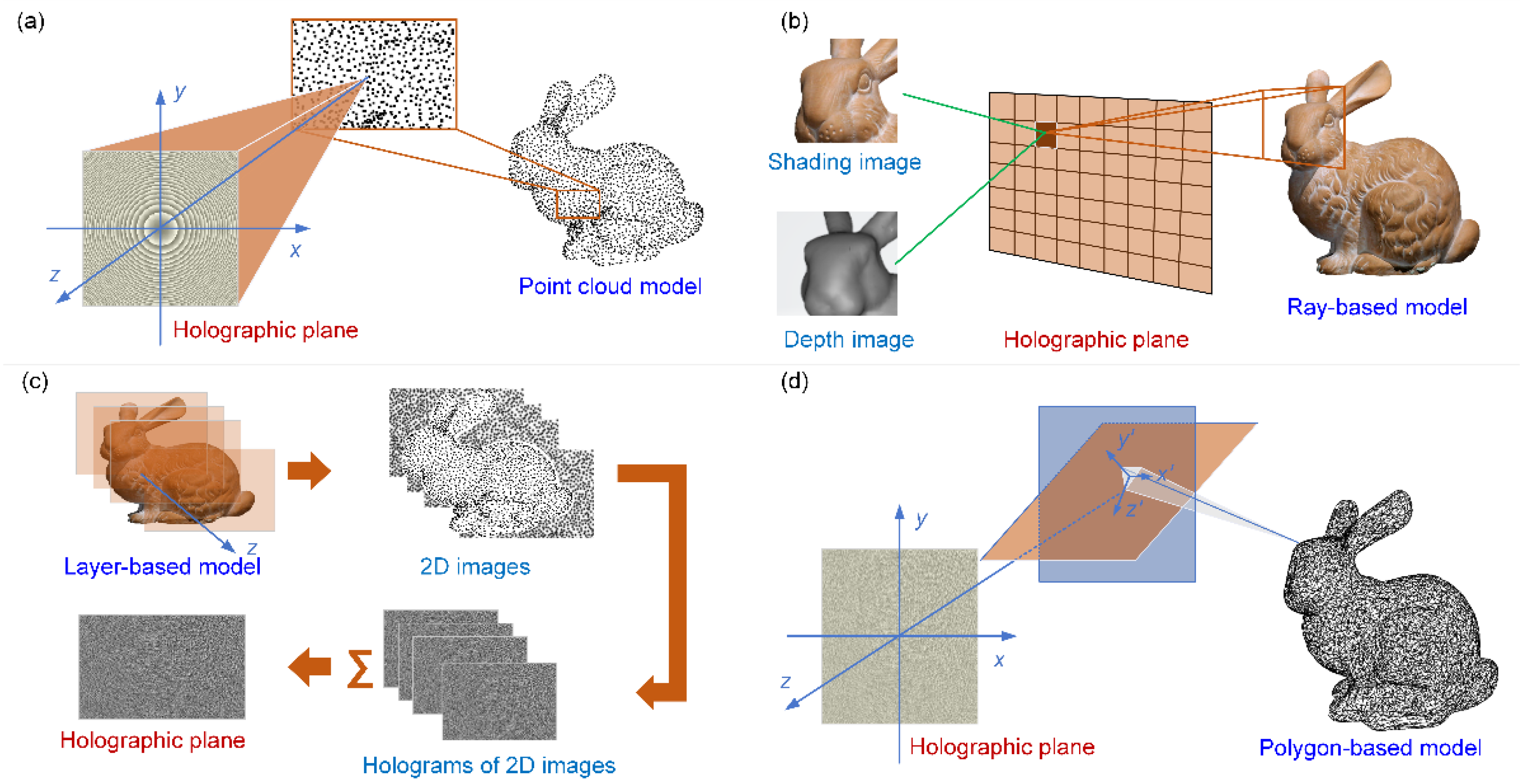
Compared with traditional optical holography, CGH has obvious advantages, such as the ability to reconstruct virtual scenes and dynamic sceneries [18]. The CGH algorithms based on physical simulation can be divided into the point–based method, the ray–based method, the polygon–based method, and the layer–based method. The hologram synthesis from different primitives is shown in Figure 1.

Figure 1.
Hologram synthesis from different primitives: (a) point–based CGH method; (b) ray–based CGH method; (c) layer–based CGH method; and (d) polygon–based CGH method.
The point–based CGH method is based on the Huygens–Fresnel principle [32]. The model of a three–dimensional scene is sampled into the three–dimensional point array with N points. Then, every point is regarded as a point light source that emits spherical waves. The complex amplitude distribution of each point on the hologram plane is added up to get the final complex amplitude hologram. The optical field in the hologram plane from one single point can be described by
where is the wavelength; stands for the complex amplitude of the object point; and , , and represent the spatial coordinates of the point. The long calculation time is an obvious shortcoming of this method. In the ray–based method, the object is prepared based on the spatial–angular distribution of the target light rays. The hologram plane is divided into several sections of equal size, and the section–wise processing is conducted. The corresponding light field is Fourier–transformed after it is multiplied by the random phase distribution. Then, the optical information propagated to the hologram plane is synthesized numerically to obtain the final hologram. In the polygon–based method, the object is processed as the polygon mesh form. The optical field of each triangular facet is calculated and accumulated in the hologram plane. The calculation of the triangular facet is performed by finding the relationship between the angular spectrum in the hologram plane and the triangular facet. The layer–based method divides the object scene into N layers and calculates the propagation of each layer. Compared with the point–based method, this method can effectively reduce the calculation amount and improve the image quality [33,34,35].
However, physical simulation has a huge drawback: it is difficult to deal with occlusion in 3D scenes. To address this issue, the holographic stereogram is introduced. In this method, the hologram space is segmented into multiple hologram primitives. The parallax of different primitives is analyzed from different angles by synthesis. However, the depth information is partially missing [36,37,38]. With regard to the encoding part, the complex amplitude distribution on the hologram plane is converted into an amplitude–only or phase–only hologram. Some common encoding methods include the bipolar amplitude encoding method, phase encoding method, and binary encoding method. After encoding, the hologram can be uploaded to the SLM and illuminated with a coherent light to reconstruct the object. For the point–based, ray–based, layer–based, and polygon–based methods, it is still a big challenge to realize real–time computing. The tradeoff between the computation time and reconstruction quality limits the practical application of CGH. Therefore, the deep learning methods are introduced into the hologram generation process because of their good performance in both accuracy and calculation speed.
3. Network Structures
Once the neural network and mathematical model (MCP model) were proposed by McCulloch et al. [39], artificial neural networks began to develop gradually. In 2012, Alex et al. proposed the first deep convolutional neural network (CNN), called AlexNet [40]. Since then, the deep learning network has been improving rapidly. In the field of information optics, many CNNs have been proposed and used in related works, such as holographic reconstruction, lensless imaging, and phase imaging. The basic neural networks commonly used in CGH are introduced as follows.
3.1. U–Net
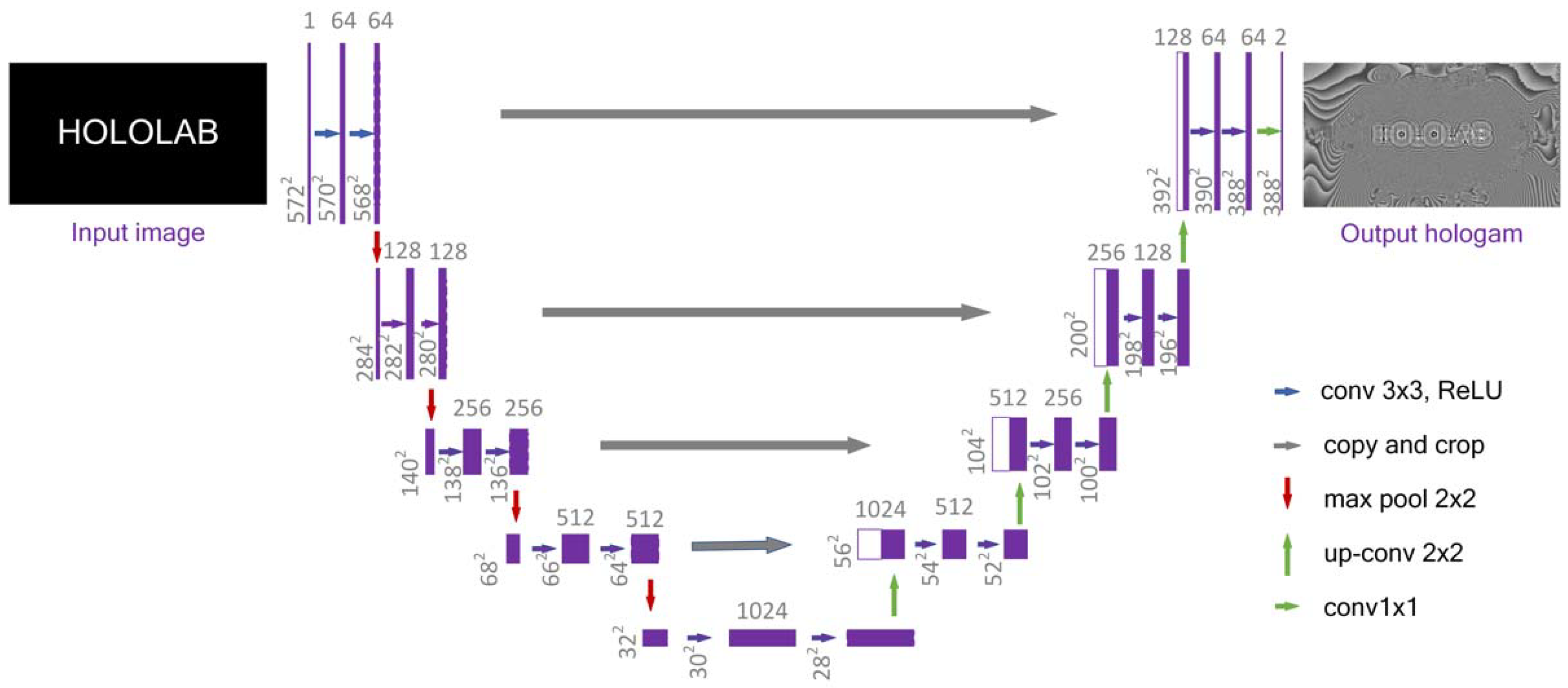
U–Net was initially proposed to solve the problem of image recognition and segmentation. In this area, the fully convolutional network (FCN) was the first representative of pixel–level image classification and semantic–level image segmentation [41]. With the improvements and developments of FCN, Ronneberger et al. improved the network structure by expanding the capacity of the network decoder. A contracting path between the encoder and decoder was added to achieve more accurate pixel boundary positioning [22]. U–Net is a kind of FCN structure. Furthermore, Milletari et al. proposed V–Net in 2016 [42]. V–Net can be understood as a 3D version of U–Net, which is suitable for medical image segmentation of 3D structures. There are also some other U–Net–based networks. For example, Jegou et al. proposed a variant network by adding dense connection blocks, called DenseNet [43].
U–Net is a U–shaped network structure that obtains context information and location information. It is a commonly used segmentation model, which is simple, efficient, easy to build, and can be trained with small datasets. The structure is shown in Figure 2. The input image is what we want to process, while the output map represents the recognition and segmentation of the input. The structure consists of a contraction down–sampling path for feature extraction (left) and an up–sampling expansion path for reconstruction (right).
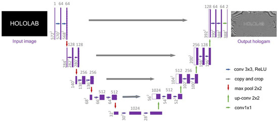
Figure 2.
Structure of the U–Net neural network.
In the early works of U–net, the left half network consists of repeated 3 × 3 convolutions (unpadded convolutions). Each convolution operation is followed by a correction linear unit (ReLU) and a 2 × 2 maximum pool operation. At each down–sampling step, the number of feature channels is doubled. Each step in the up–sampling expansion path consists of a 2 × 2 up–convolution and two 3 × 3 convolutions followed by a ReLU. It halves the feature channel number and concatenates with the corresponding cropped feature map in the contraction path. Clipping is required because of the loss of border pixels in every convolution operation. The total number of convolution layers is 23 [22].
U–Net has become the baseline for most semantic segmentation tasks, which has also inspired a large number of researchers to think about the U–shaped network. For multi–modal images, U–Net can extract the features of different modes. The images processed by U–Net have simple semantics and fixed structure, and fewer data are required for U–Net. However, when the image is complex, its performance is greatly reduced. Compared with many current networks, U–Net has fewer layers and fewer parameters, so it is easy to overfit the datasets during the training process. Changing the original simple structure into DenseNet can increase the hyperparameters in the network [43]. At the same time, using transfer learning and loading training weights can also improve network performance. Thus, U–Net was firstly considered for CGH calculation and gradually revised or replaced by other advanced networks, such as ResNet or GAN.
3.2. ResNet
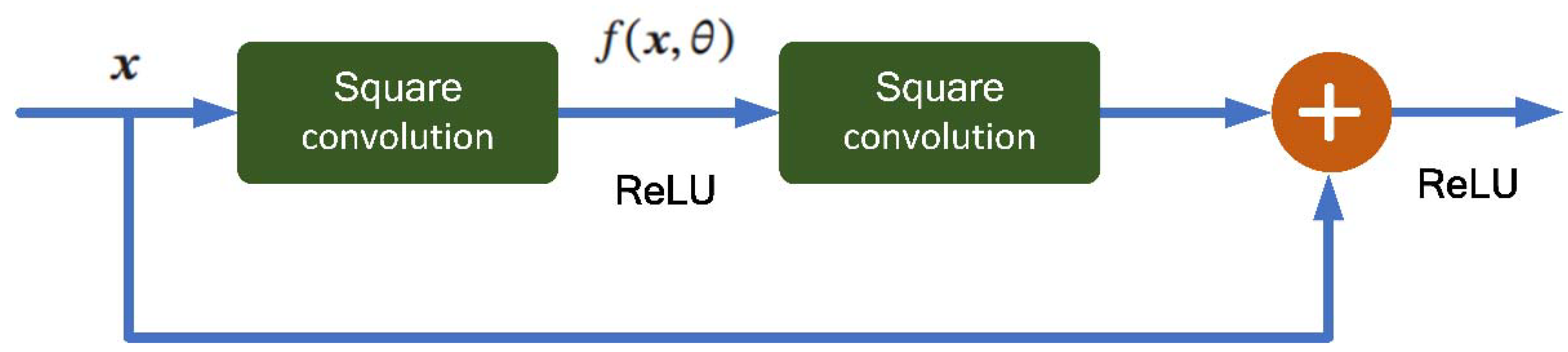
ResNet improves the transmission efficiency of information by adding a shortcut connection to the nonlinear convolution layer. Many “highway networks” present shortcut connections with gating functions, while the identity shortcuts of ResNet are parameter–free. Thus, the shortcuts are never closed and all information can pass through the whole network [44,45,46]. The ResNet reformulates the layers as learning residual functions with reference to the layer inputs. The networks are easier to optimize and can gain high accuracy from considerably increased depth. It is like U–Net and adds the calculation of some residual blocks. Suppose that in a depth network we can expect a nonlinear element convolution layer to approximate an objective function , which can be divided into two parts, the identity function and residual function . Then we can define it as
According to the general approximation principle, a nonlinear element composed of a neural network has enough ability to approximate the original objective function or residual function while the latter is better to be learned [46]. Thus, the original optimization problem can be transformed into the idea that we make the nonlinear element approximate the residual function and approximate . A simple unit of the ResNet is shown in Figure 3. The typical residual element is composed of multiple convolution layers with equal width and a direct edge across the layer. Moreover, the output is obtained after the activation by ReLU.
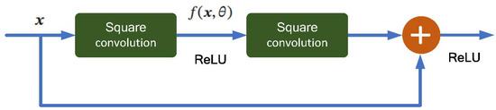
Figure 3.
The residual element block structure.
ResNet is a deep neural network composed of many residual blocks in series. It solves the gradient vanishing problem when the network depth increases to a certain extent. It can make the feedforward or feedback propagation algorithm go smoothly and the structure is simpler. The increase in identity mapping cannot reduce the performance of the network. Thus, the ResNet is suitable for the CGH generation after being trained.
3.3. GAN
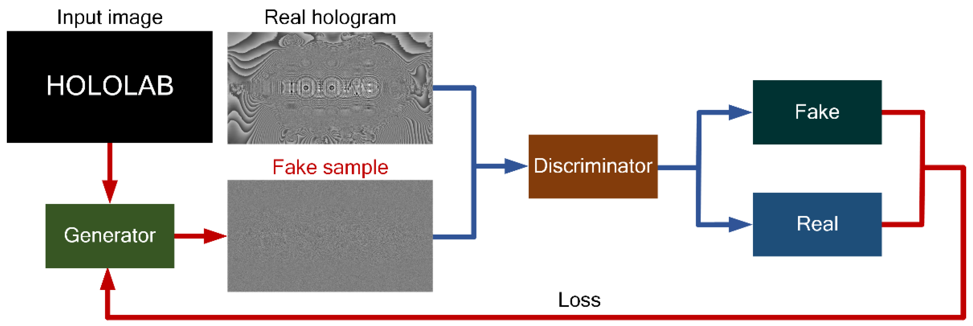
With the gradual development of deep learning, different network structures have been proposed. In order to reduce the needed datasets for training, the GAN structure was proposed. In 2014, Ian et al. proposed the GAN network, which can be seen as a zero–sum game. After that, the research group reviewed the applications of GANs and identified the core research problems to make GANs a reliable technology in 2020 [47].
The GAN methods make the samples generated by the generated network obey the real data distribution through confrontation training. The GAN structures include two sub–networks for adversarial training. One is called the generator and the other is called the discriminator. The structure is shown in Figure 4. The discriminator is used to accurately determine whether a sample is from real data or generated by the generator, while the generator is used to generate samples from sources that cannot be distinguished by the discriminator. In the following, how GAN conducts generative confrontation is demonstrated.
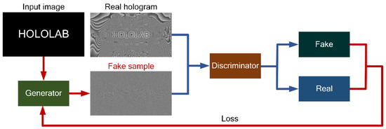
Figure 4.
Structure of GAN.
The function of the discriminator network is to distinguish whether the sample is from true distribution or the generated model . Therefore, is a binary classifier. indicates that the sample comes from the true distribution, and indicates that the sample comes from the generator. The value of represents the probability that the sample is the distribution of real data. The model can be formulated as
Given the sample , indicates whether it comes from or , and the objective function is to minimize the cross entropy, formulated as
If is mixed with and in equal proportions, then . Equation (4) can be equivalent to the following equation:
In Equation (5), g and are the parameters of the generator and discriminator, respectively. The goal of the generator is opposite that of the discriminator. It aims to make the discriminator distinguish the samples generated by the generator from real samples. The model can be defined as
We combine the two networks as a whole and regard them as the minimax game, which can be defined as
If and are known, the optimal discriminator can be defined as
The GAN method is a kind of semi–supervised method to train classifiers [48]. The parameter update of the generator is not obtained directly from the data sample but by using the backpropagation from the discriminator. Thus, it can reduce the number of samples and generate samples faster. However, compared with the single objective optimization, the training of GANs is difficult and unstable because it is necessary to balance the capabilities of the two networks. Thus, for the CGH calculation, we need to keep the generator value constant when training the discriminator, and vice versa. Each discriminator and generator should be trained against a static opponent for a slightly higher effect than the previous iterations.
4. The Learning–Based CGH
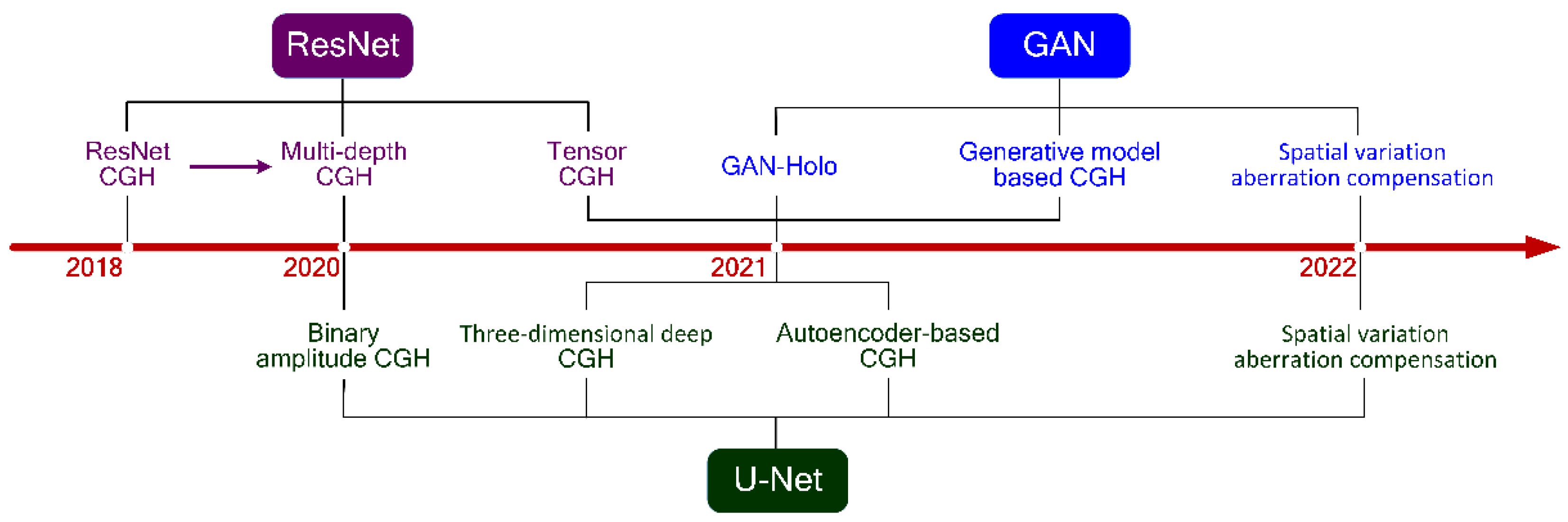
In this section, having introduced the CGH principle and some of the common deep learning networks in the second and third sections, we review the recent studies on the applications of deep learning networks in CGH. As is shown in Figure 5, the developments and applications of CGH using deep learning in recent years are presented. We can see the rapid rise of the learning–based CGH. Moreover, we compare the methods and research results of holography based on the networks, as shown in Table 1.

Figure 5.
Development and application of CGH based on DNN in recent years.

Table 1.
DNN used in CGH based on deep learning.
4.1. ResNet and U–Net Based Deep CGH
The U–Net neural network has few layers and parameters and is easy to be trained. ResNet and U–Net–based deep CGHs have been developed. In 2018, Horisaki et al. used a deep ResNet for calculating holograms [23]. Their training dataset was composed of uniform random phase patterns and their Fresnel propagating patterns at a distance. The number of training speckle pairs was 100,000.
Then, for less computation and faster generation speed, Goi et al. proposed a U–Net–based architecture to generate binary holograms [24]. The DenseNet architecture was used to find a better solution. The output gradient of each block in the front was skip–connected to the output of each block in the back. A similar selective structure was added to the same layer to further improve the effect. In this method, random amplitude binary patterns and their Fresnel propagating intensity patterns were used for the network training. The pixel number of the hologram and target pattern was 128 × 128. The number of the training dataset was 10,000. Numerical and optical experiments were carried out, and the proposed method was compared with the Fresnel ping–pong method in terms of quality and calculation time. The training of the proposed method took 6000 s for preparation and 0.03 s for each hologram, while the ping–pong method took 0.7 s per hologram.
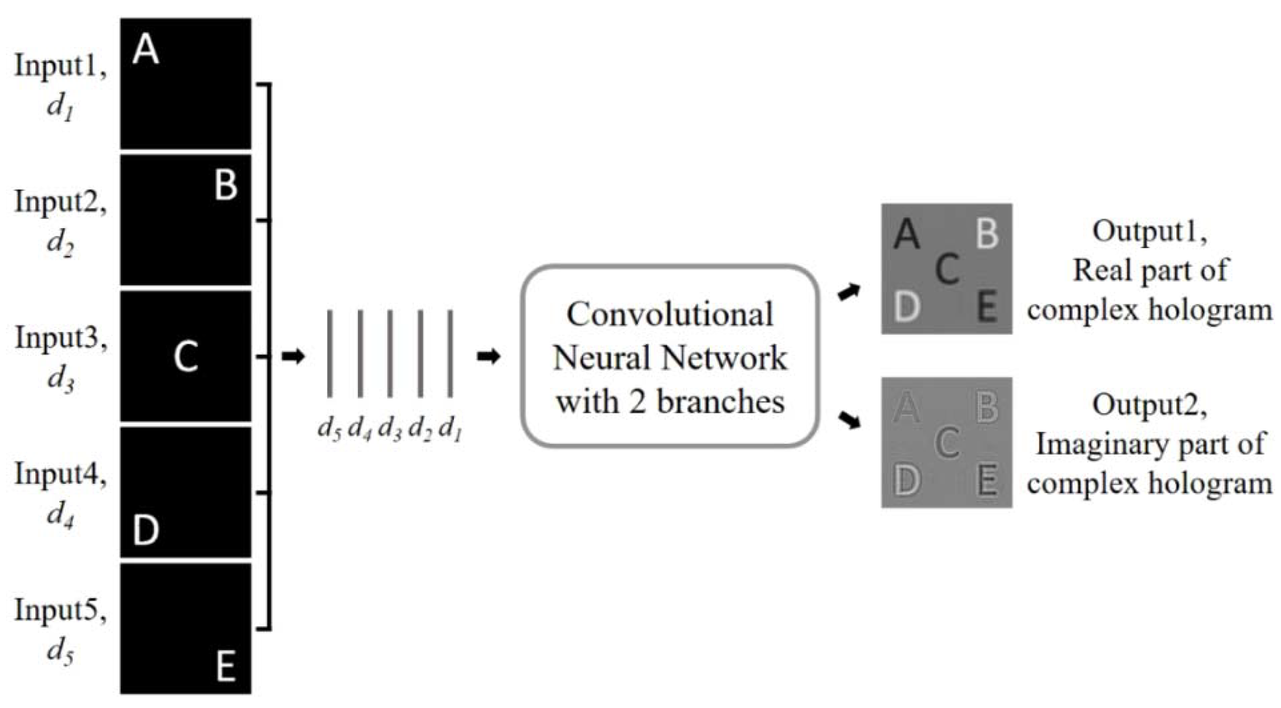
The algorithms above realized better and faster reconstruction of the two–dimensional image through deep learning networks. To realize the reconstruction of 3D images, Lee et al. presented a deep neural network for generating a multi–depth hologram in 2020, as shown in Figure 6 [29]. The proposed multi–depth hologram generation network (MDHGN) receives multiple images with different depths as input and generates complex holograms that can reconstruct the input images. According to each depth of d1 to d5, five different images of randomly positioned dots were generated and superimposed as a 3D target. The complex hologram calculated by the ASM algorithm was divided into a real hologram and an imaginary hologram, and stored as the ground truth. NVIDIA’S Quadro P5000 GPU was used to train the network. The numerical and optical reconstructions were carried out, which proved that it is possible to reconstruct multiple images at different depths [29].
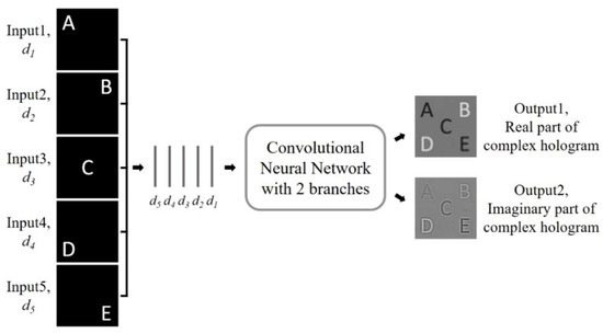
Figure 6.
Overall schematic diagram of the MDHGN. Multiple intensity profiles are concatenated in the channel axis and provided as input data. The MDHGN generates a multi–depth complex hologram from the inputs. The real and imaginary parts of the complex hologram are calculated, respectively. (Adapted from [29]).
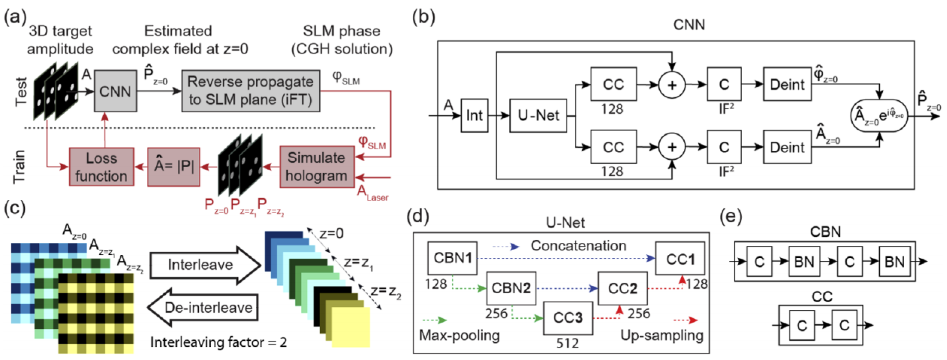
In 2020, Eybposh et al. proposed a new algorithm, DeepCGH, for hologram synthesis [49]. The concept map of DeepCGH is shown in Figure 7. The unsupervised training method was employed in order to overcome the limitation of the training dataset. The network architecture of DeepCGH was U–Net with five convolutional blocks. The proposed method was compared with the GS and NOVO–CGH algorithms. DeepCGH was implemented in the Python programming language using TensorFlow 2.0 deep learning framework. The models were trained with NVIDIA GeForce RTX 2080Ti GPUs, while the GS and NOVO–CGH algorithms were implemented with MATLAB and CUDA GPU libraries. It was presented that the 3D holograms synthesized with DeepCGH had greater accuracy, and the processing speed was higher than that of the existing methods.

Figure 7.
(a) Trained CNN estimates the complex field in the image plane. (b) CNN structure for DeepCGH. (c) The interleave module and the de–interleave module. (d) The U–Net model containing two types of convolutional blocks. (e) CCn and CBNn convolutional blocks. (Adapted from [49]).
Then, in 2021, based on the ResNet, Horisaki et al. proposed a noniterative 3D CGH method to reproduce a 3D intensity pattern in a given class. The U–Net was the main network framework of this method. The 3D target patterns were images of handwritten digits randomly selected from the EMNIST dataset. The number of the training dataset images was 279,600. The network was trained and tested on an Intel Xeon 6134 CPU @ 3.2 GHz with 192 GB of RAM and an NVIDIA Tesla V100 GPU with 16 GB of VRAM [5,51]. The deep learning method was compared with the GS method and proved the effectiveness for 3D image reconstruction.
In the same year, the concept of tensor holography for true 3D color holography was proposed by Shi et al. [50]. Their network architecture consisted of residual blocks and a skip connection from the input to the penultimate residual block. A large–scale Fresnel hologram dataset, called MIT–CGH–4K, which consists of 4000 pairs of RGB–depth (RGB–D) images and their corresponding 3D holograms, was used for the training of the CNN. They trained the CNN on an NVIDIA Tesla V100 GPU for 84 h. The trained model was well extended to computer rendering, real–world captured RGB–D input, and the standard test mode. The tensor holography method was compared with U–Net and Dilated–Net, and it achieved the highest performance when the configuration was the same as that of the other two models.
4.2. GAN–Based Deep CGH
In addition to the ResNet–based networks and U–Net–based networks, it is also effective to use a GAN network to cut down the huge calculation time of the iterative CGH methods. GAN networks have gained a lot of attention in the computer vision community due to their data generation capability without explicitly modeling the probability density function [52].
In 2020, Khan et al. proposed a new method using GAN–based DNN for holography. The framework consisted of two phases. In phase one, the Fresnel–based method was used to make the dataset. In phase two, the raw input image and holographic label image data from phase one acquired images were trained to improve the accuracy and efficiency. The training dataset was composed of the handwritten digit dataset and its corresponding holograms. The label holograms, as the ground truth, were generated by the Fresnel method. To generate a single hologram, an Intel Core™ i7–7820X CPU @ 3.60 GHz and a GeForce GTX 1080 (NVIDIA) were used. The training time for GAN–Holo was 20 h. The computational time based on GAN–Holo and the Fresnel method was 5 ms and 94 ms, respectively. The root mean square error (RMSE) between the reconstructed images and target intensity patterns obtained by the proposed method was below 0.1, which performed fairly well [27].
In 2021, to improve the reconstruction quality, Kang et al. proposed a GAN–based DNN for fringe pattern generation. The fake data were inferred using the DNN–based fringe pattern generator and compared with the real data by using the discriminator. Then, the parameters of the discriminator and generator were updated simultaneously. By repeating this process, the real and fake became indistinguishably similar. NVIDIA Tesla V100 (32 Gb) and Intel Xeon Gold 5120@2.20 GHz were used as the GPU and CPU. Two datasets of 16 and 32 spaces were constructed by using object points that existed within a certain space for training. It took about 520 h and 1944 h for the 16 and 32 spaces to learn the real and imaginary parts, respectively. After completing the training, it took 360 µs to generate a fringe pattern for each one. The average PSNR in the 16 space was 44.56 dB, and the average PSNR in the 32 space was 35.11 dB [25]. The training process was time–consuming, but the CGH calculation after the training was very fast with a relatively high PSNR.
Aiming to generate a hologram with spatially varying aberration compensation, Yoo et al. proposed a new method using a combination of an FFT–based convolution and a neural network [26]. The optical aberrations of the holographic display were denoted. The training dataset was composed of pairs of various images and corresponding aberration compensation maps. The compensation maps were synthesized by the pointwise integration method. Then, a propagator was designed to reconstruct an image close to the target image. The NVIDIA Tesla P40 GPU with a 24 GB memory was used for the generation and the 800 training images of the DIV2K dataset were exploited as the target images. The parameters of the generator were optimized by using the dataset and the results of the propagator. The main network in the propagator was U–Net and the general idea of the proposed propagator was based on GAN. The optical experiments verified the performance of the technique for aberration compensation.
4.3. Autoencoder–Based CGH
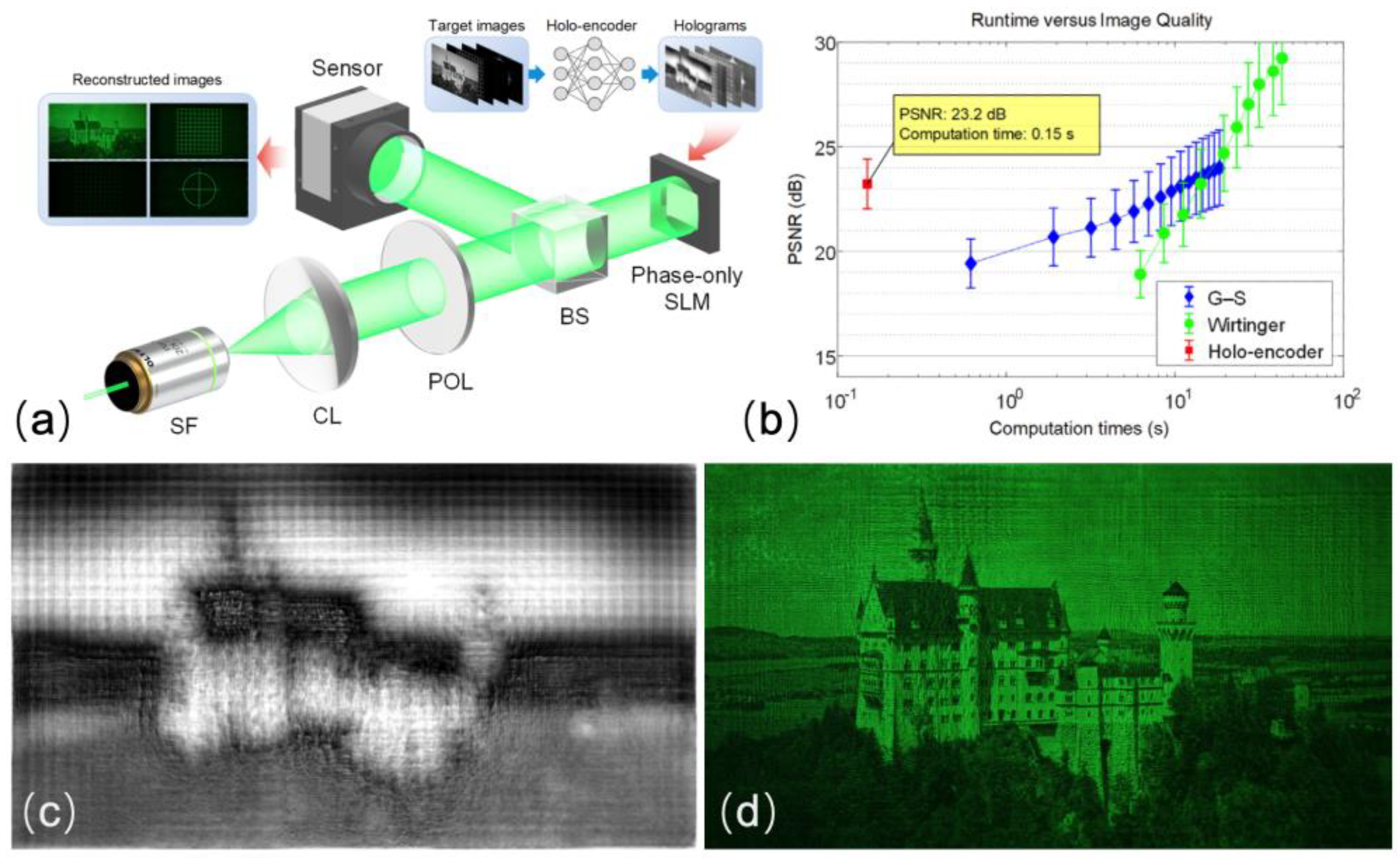
In addition to all the works above, Wu et al. proposed an autoencoder–based neural network for phase–only hologram generation, called Holo–Encoder [10]. It incorporated the Fresnel diffraction model into the network framework to realize the unsupervised training. The network was trained for 10 epochs using an Adam optimizer and the training images were obtained from the DIV2K dataset. The problem of gradient disappearance in deep learning training could be solved by adding the residual to U–Net. Using a combination of negative Pearson correlation coefficient (NPCC), perception loss function, and TV regularization, the training results were constrained from three aspects: pixel–wise, feature–wise, and smoothness of phase. The Holo–Encoder was compared with the GS holography and the Wirtinger holography. All three algorithms were run on the same workstation with a Xeon CPU E5–2650 (2.20 GHz) and 128 GB of RAM. An NVIDIA Quadro GV100 GPU was used for the prediction of the Holo–Encoder. As shown in Figure 8, a smoother phase hologram and a better reconstructed image were obtained, while the computation time was only 0.15 s, outperforming other methods with regard to the runtime.

Figure 8.
(a) Experimental setup of the Holo–Encoder. (b) Evaluation of the algorithm running time and reconstruction quality. (c) POH predicted by the Holo–Encoder. (d) Experimental reconstruction of (c). (Adapted from [10]).
4.4. Loss Function, Dataset, and GPU or CPU
Loss function is a significant part of the training process that governs the network performance. Different loss functions lead to significant performance differences. The popular loss functions used in the learning–based CGH are mean square error (MSE) or root mean square error (RMSE). The MSE function measures the reconstruction quality by calculating the square of the error between the predicted value and the ground truth. The closer the predicted value and the ground truth are, the smaller the mean square is. The MSE can be defined as
For the GAN network, its generator and discriminator need two loss functions. The GAN uses a binary cross entropy loss function to train D and G. The D and G are opposed to each other till the convergence. Combined loss functions were also proposed for the comprehensive constraints. For example, Holo–Encoder uses the NPCC and perceptual loss function. The training results are constrained from both the pixel–by–pixel aspect and the overall aspect [10]. The MDHGN uses the MSE and L1 loss to compare the target and reconstruction images [29]. Moreover, tensor holography introduces two wave–based loss functions to train the CNN for an accurate hologram. The first loss function measures the data fidelity, and the second loss function measures the perceptual quality of the reconstructed 3D scene [50]. The definitions of different loss functions are presented in Table 2 and the loss functions used in the CGH generation tasks are summarized in Table 3, respectively.
Table 2.
The definition of loss functions.
Table 3.
The loss functions for deep–learning–based CGH.
Moreover, it is important to have a good dataset and a suitable GPU for network training. The DIV2K dataset is a popular training dataset in the above learning–based CGH tasks [10,26]. The DIV2K dataset is a super–resolution reconstruction dataset, which is large enough to avoid the simple overfit. There are 1000 high–definition 2K images, including 800 for training, 100 for verification, and 100 for testing. A CPU running @ 3.20 GHz with 128 GB of RAM and NVIDIA Tesla V100 (32 Gb) are expected for the aforementioned algorithms [10,25,26,50].
5. Conclusions and Outlook
In conclusion, through the analysis of CGH based on the four network structures, including U–Net, ResNet, GAN, and autoencoder, we summarized the characteristics of each form. Compared with U–Net, ResNet introduces the residual block so that the output feature map is more sensitive to the changes. It can effectively solve the gradient disappearance problem. Compared with U–Net and ResNet, GAN can be used to construct a discriminator and generator of various differentiable functions. However, it is difficult to train, as the discriminator and generator need to be well synchronized. The autoencoder–based deep CGH can automatically learn the latent encodings of CGH and make full use of the neural network advantages.
It is suggested that advanced network architectures and smart mapping relations can be applied to obtain faster calculation and higher reconstruction quality. Moreover, more efforts are expected to accelerate the calculation in the future. Several network frameworks including physical models need to be further optimized to ensure high–fidelity optical reconstruction. Deep learning opens a new door for possible real–time CGH calculation. Along with the developments of the advanced deep networks, we believe that deep learning could be a universal solution to the CGH calculation as well as the DOE and metasurface design in the field of diffractive optics.
Author Contributions
Conceptualization, Y.Z. and M.Z.; investigation, Y.Z. and M.Z.; supervision, L.C.; writing—original draft preparation, Y.Z.; writing—review and editing, Y.Z., M.Z., K.L., Z.H. and L.C. All authors have read and agreed to the published version of the manuscript.
Funding
This research was funded by National Natural Science Foundation of China (NSFC), grant number 62035003, and the China Postdoctoral Science Foundation, grant number BX2021140.
Institutional Review Board Statement
Not applicable.
Informed Consent Statement
Not applicable.
Data Availability Statement
All data generated or analyzed during this study are included in this published article.
Conflicts of Interest
The authors declare no conflict of interest.
References
- He, Z.; Sui, X.; Zhang, H.; Jin, G.; Cao, L. Frequency-based optimized random phase for computer-generated holographic display. Appl. Opt. 2021, 60, A145–A154. [Google Scholar] [CrossRef] [PubMed]
- Wang, D.; Liu, C.; Shen, C.; Xing, Y.; Wang, Q.H. Holographic capture and projection system of real object based on tunable zoom lens. PhotoniX 2020, 1, 6. [Google Scholar] [CrossRef]
- Zhao, Y.; Cao, L.; Zhang, H.; Tan, W.; Wu, S.; Wang, Z.; Yang, Q.; Jin, G. Time-division multiplexing holographic display using angular-spectrum layer-oriented method (Invited Paper). Chin. Opt. Lett. 2016, 14, 010005. [Google Scholar] [CrossRef]
- He, Z.; Sui, X.; Jin, G.; Cao, L. Progress in virtual reality and augmented reality based on holographic display. Appl. Opt. 2019, 58, A74–A81. [Google Scholar] [CrossRef]
- Horisaki, R.; Nishizaki, Y.; Kitaguchi, K.; Saito, M.; Tanida, J. Three-dimensional deeply generated holography [Invited]. Appl. Opt. 2021, 60, A323–A328. [Google Scholar] [CrossRef]
- Wu, L.; Zhang, Z. Domain multiplexed computer-generated holography by embedded wavevector filtering algorithm. PhotoniX 2021, 2, 1. [Google Scholar] [CrossRef]
- Wang, Z.; Zhang, X.; Lv, G.; Feng, Q.; Ming, H.; Wang, A. Hybrid holographic Maxwellian near-eye display based on spherical wave and plane wave reconstruction for augmented reality display. Opt. Express 2021, 29, 4927–4935. [Google Scholar] [CrossRef]
- Wang, Z.; Zhang, X.; Tu, K.; Lv, G.; Feng, Q.; Wang, A.; Ming, H. Lensless full-color holographic Maxwellian near-eye display with a horizontal eyebox expansion. Opt. Lett. 2021, 46, 4112–4115. [Google Scholar] [CrossRef]
- Sui, X.; He, Z.; Jin, G.; Chu, D.; Cao, L. Band-limited double-phase method for enhancing image sharpness in complex modulated computer-generated holograms. Opt. Express 2021, 29, 2597–2612. [Google Scholar] [CrossRef]
- Wu, J.; Liu, K.; Sui, X.; Cao, L. High-speed computer-generated holography using an autoencoder-based deep neural network. Opt. Lett. 2021, 46, 2908–2911. [Google Scholar] [CrossRef]
- Yamaguchi, I.; Zhang, T. Phase-shifting digital holography. Opt. Lett. 1997, 22, 1268–1270. [Google Scholar] [CrossRef] [PubMed]
- Cuche, E.; Bevilacqua, F.; Depeursinge, C. Digital holography for quantitative phase-contrast imaging. Opt. Lett. 1999, 24, 291–293. [Google Scholar] [CrossRef] [PubMed]
- Sinclair, G.; Jordan, P.; Courtial, J.; Padgett, M.; Cooper, J.; Laczik, Z.J. Assembly of 3-dimensional structures using programmable holographic optical tweezers. Opt. Express 2004, 12, 5475–5480. [Google Scholar] [CrossRef] [PubMed]
- Matsushima, K.; Schimmel, H.; Wyrowski, F. Fast calculation method for optical diffraction on tilted planes by use of the angular spectrum of plane waves. J. Opt. Soc. Am. A 2003, 20, 1755–1762. [Google Scholar] [CrossRef]
- Sakata, H.; Sakamoto, Y. Fast computation method for a Fresnel hologram using three-dimensional affine transformations in real space. Appl. Opt. 2009, 48, H212–H221. [Google Scholar] [CrossRef]
- Ogihara, Y.; Ichikawa, T.; Sakamoto, Y. Fast calculation with point-based method to make CGHs of the polygon model. In Proceedings of the SPIE—The International Society for Optical Engineering, San Francisco, CA, USA, 1–6 February 2014; Volume 9006. [Google Scholar]
- Zhang, Y.; Fan, H.; Wang, F.; Gu, X.; Qian, X.; Poon, T.C. Polygon-based computer-generated holography: A review of fundamentals and recent progress [Invited]. Appl. Opt. 2022, 61, B363–B374. [Google Scholar] [CrossRef]
- Zhao, Y.; Cao, L.; Zhang, H.; Kong, D.; Jin, G. Accurate calculation of computer-generated holograms using angular-spectrum layer-oriented method. Opt. Express 2015, 23, 25440–25449. [Google Scholar] [CrossRef]
- Wei, H.; Gong, G.; Li, N. Improved look-up table method of computer-generated holograms. Appl. Opt. 2016, 55, 9255–9264. [Google Scholar] [CrossRef]
- Ju, Y.G.; Park, J.H. Foveated computer-generated hologram and its progressive update using triangular mesh scene model for near-eye displays. Opt. Express 2019, 27, 23725–23738. [Google Scholar] [CrossRef]
- Wei, L.; Sakamoto, Y. Fast calculation method with foveated rendering for computer-generated holograms using an angle-changeable ray-tracing method. Appl. Opt. 2019, 58, A258–A266. [Google Scholar] [CrossRef]
- Ronneberger, O.; Fischer, P.; Brox, T. U-Net: Convolutional Networks for Biomedical Image Segmentation. In Proceedings of the Medical Image Computing and Computer-Assisted Intervention—MICCAI 2015, Munich, Germany, 5–9 October 2015; pp. 234–241. [Google Scholar]
- Horisaki, R.; Takagi, R.; Tanida, J. Deep-learning-generated holography. Appl. Opt. 2018, 57, 3859–3863. [Google Scholar] [CrossRef] [PubMed]
- Goi, H.; Komuro, K.; Nomura, T. Deep-learning-based binary hologram. Appl. Opt. 2020, 59, 7103–7108. [Google Scholar] [CrossRef] [PubMed]
- Kang, J.W.; Park, B.S.; Kim, J.K.; Kim, D.W.; Seo, Y.H. Deep-learning-based hologram generation using a generative model. Appl. Opt. 2021, 60, 7391–7399. [Google Scholar] [CrossRef]
- Yoo, D.; Nam, S.W.; Jo, Y.; Moon, S.; Lee, C.K.; Lee, B. Learning-based compensation of spatially varying aberrations for holographic display [Invited]. J. Opt. Soc. Am. A 2022, 39, A86–A92. [Google Scholar] [CrossRef] [PubMed]
- Khan, A.; Zhijiang, Z.; Yu, Y.; Khan, M.A.; Yan, K.; Aziz, K. GAN-Holo: Generative Adversarial Networks-Based Generated Holography Using Deep Learning. Complexity 2021, 2021, 6662161. [Google Scholar] [CrossRef]
- Feng, W.; Sun, X.; Li, X.; Gao, J.; Zhao, X.; Zhao, D. High-speed computational ghost imaging based on an auto-encoder network under low sampling rate. Appl. Opt. 2021, 60, 4591–4598. [Google Scholar] [CrossRef] [PubMed]
- Lee, J.; Jeong, J.; Cho, J.; Yoo, D.; Lee, B.; Lee, B. Deep neural network for multi-depth hologram generation and its training strategy. Opt. Express 2020, 28, 27137–27154. [Google Scholar] [CrossRef]
- Blinder, D.; Birnbaum, T.; Ito, T.; Shimobaba, T. The state-of-the-art in computer generated holography for 3D display. Light Adv. Manuf. 2022, 3, 35. [Google Scholar] [CrossRef]
- Shimobaba, T.; Blinder, D.; Birnbaum, T.; Hoshi, I.; Shiomi, H.; Schelkens, P.; Ito, T. Deep-Learning Computational Holography: A Review (Invited). Front. Phys. 2022, 3, 854391. [Google Scholar] [CrossRef]
- Shimobaba, T.; Ito, T.; Masuda, N.; Ichihashi, Y.; Takada, N. Fast calculation of computer-generated-hologram on AMD HD5000 series GPU and OpenCL. Opt. Express 2010, 18, 9955–9960. [Google Scholar] [CrossRef] [Green Version]
- Youchao, W.; Daoming, D.; Peter, J.C.; Andrew, K.; Ralf, M.; Fan, Y.; Timothy, D.W. Hardware implementations of computer-generated holography: A review. Opt. Eng. 2020, 59, 102413. [Google Scholar] [CrossRef]
- Slinger, C.; Cameron, C.; Stanley, M. Computer-generated holography as a generic display technology. Computer 2005, 38, 46–53. [Google Scholar] [CrossRef]
- Park, J.H. Recent progress in computer-generated holography for three-dimensional scenes. J. Inf. Disp. 2017, 18, 1–12. [Google Scholar] [CrossRef]
- Yatagai, T. Stereoscopic approach to 3-D display using computer-generated holograms. Appl. Opt. 1976, 15, 2722–2729. [Google Scholar] [CrossRef]
- St Hilaire, P. Modulation transfer function and optimum sampling of holographic stereograms. Appl. Opt. 1994, 33, 768–774. [Google Scholar] [CrossRef]
- McCrickerd, J.T.; George, N. Holographic stereogram from sequential component photographs. Appl. Phys. Lett. 1968, 12, 10–12. [Google Scholar] [CrossRef]
- McCulloch, W.S.; Pitts, W. A logical calculus of the ideas immanent in nervous activity. Bull. Math. Biol. 1990, 52, 99–115. [Google Scholar] [CrossRef]
- Krizhevsky, A.; Sutskever, I.; Hinton, G.E. ImageNet classification with deep convolutional neural networks. Commun. ACM 2017, 60, 84–90. [Google Scholar] [CrossRef]
- Shelhamer, E.; Long, J.; Darrell, T. Fully Convolutional Networks for Semantic Segmentation. IEEE Trans. Pattern Anal. Mach. Intell. 2017, 39, 640–651. [Google Scholar] [CrossRef]
- Milletari, F.; Navab, N.; Ahmadi, S. V-Net: Fully Convolutional Neural Networks for Volumetric Medical Image Segmentation. In Proceedings of the 2016 Fourth International Conference on 3D Vision (3DV), Stanford, CA, USA, 25–28 October 2016; pp. 565–571. [Google Scholar]
- Jégou, S.; Drozdzal, M.; Vázquez, D.; Romero, A.; Bengio, Y. The One Hundred Layers Tiramisu: Fully Convolutional DenseNets for Semantic Segmentation. In Proceedings of the 2017 IEEE Conference on Computer Vision and Pattern Recognition Workshops (CVPRW), Honolulu, HI, USA, 21–26 July 2017; pp. 1175–1183. [Google Scholar]
- He, K.; Sun, J. Convolutional neural networks at constrained time cost. In Proceedings of the 2015 IEEE Conference on Computer Vision and Pattern Recognition (CVPR), Boston, MA, USA, 7–12 June 2015; pp. 5353–5360. [Google Scholar]
- Srivastava, R.K.; Greff, K.; Schmidhuber, J. Highway Networks. arXiv 2015, arXiv:1505.00387. [Google Scholar]
- He, K.; Zhang, X.; Ren, S.; Sun, J. Deep Residual Learning for Image Recognition. In Proceedings of the 2016 IEEE Conference on Computer Vision and Pattern Recognition (CVPR), Las Vegas, NV, USA, 27–30 June 2016; pp. 770–778. [Google Scholar]
- Goodfellow, I.; Pouget-Abadie, J.; Mirza, M.; Xu, B.; Warde-Farley, D.; Ozair, S.; Courville, A.; Bengio, Y. Generative adversarial networks. Commun. ACM 2020, 63, 139–144. [Google Scholar] [CrossRef]
- Salimans, T.; Goodfellow, I.; Zaremba, W.; Cheung, V.; Radford, A.; Chen, X. Improved Techniques for Training GANs. In Proceedings of the 30th International Conference on Neural Information Processing Systems, Barcelona, Spain, 5–10 December 2016; pp. 2234–2242. [Google Scholar]
- Hossein Eybposh, M.; Caira, N.W.; Atisa, M.; Chakravarthula, P.; Pégard, N.C. DeepCGH: 3D computer-generated holography using deep learning. Opt. Express 2020, 28, 26636–26650. [Google Scholar] [CrossRef] [PubMed]
- Shi, L.; Li, B.; Kim, C.; Kellnhofer, P.; Matusik, W. Towards real-time photorealistic 3D holography with deep neural networks. Nature 2021, 591, 234–239. [Google Scholar] [CrossRef] [PubMed]
- Cohen, G.; Afshar, S.; Tapson, J.; van Schaik, A. EMNIST: Extending MNIST to handwritten letters. In Proceedings of the 2017 International Joint Conference on Neural Networks (IJCNN), Anchorage, AK, USA, 14–19 May 2017; pp. 2921–2926. [Google Scholar]
- Yi, X.; Walia, E.; Babyn, P. Generative adversarial network in medical imaging: A review. Med. Image Anal. 2019, 58, 101552. [Google Scholar] [CrossRef] [Green Version]
Publisher’s Note: MDPI stays neutral with regard to jurisdictional claims in published maps and institutional affiliations. |
© 2022 by the authors. Licensee MDPI, Basel, Switzerland. This article is an open access article distributed under the terms and conditions of the Creative Commons Attribution (CC BY) license (https://creativecommons.org/licenses/by/4.0/).