Significance of Determination Methods on Shear Modulus Measurements of Fujian Sand in Cyclic Triaxial Testing

Abstract

It has long been known that the hysteresis loops of sand under cyclic loading gradually become asymmetric with the increase of strain amplitudes, but a symmetrical hysteresis loop is widely assumed in current practice. Despite several methods which have been proposed recently to consider the hysteresis loop irregularities, previous research has lacked a quantitative study on the effects of determination methods on the shear modulus G and modulus reduction curve G/G_max. The primary objective of the current study is to evaluate the uncertainties associated with the shear modulus measurements introduced by four determination methods. Reconstituted sand specimens prepared at three relative densities are tested using strain-controlled cyclic triaxial tests, at various effective confining pressures. The results in terms of G and G/G_max with increasing shear strain are presented, following by the difference quantification in the calculated G/G_max caused by the determination methods, the G_max definition and the cycle number. The results show that the calculated G/G_max may differ significantly for the same hysteresis loop, with a maximum percentage change of 40~50%. The aggravated influence at low confining pressure highlights that careful consideration of the asymmetrical hysteresis loop at large strains is warranted.

1. Introduction

The stress–strain relationship of soils plays an important role in performing site-specific ground response analysis [1,2,3,4]. Since the one-dimensional equivalent linear method, which took into account the dynamic property of the soil has been utilized for evaluating the site response under seismic loading, extensive cyclic tests have been carried out in the laboratory to characterize the soil dynamic property for different physical properties and loading conditions.

The small-strain shear modulus G_max and the corresponding modulus reduction curve G/G_max are the two basic parameters for ground response analysis [5,6,7]. In the laboratory, several cyclic testing apparatuses can be used to measure the soil dynamic property over a wide shear strain (γ) range. For example, Hara and Kiyota [8] introduced the simple shear device which is capable of testing soils over a strain range of 10⁻⁵ to 10⁻². Isenhower [9] performed a joint use of resonant column with cyclic torsional simple shear to determine the dynamic properties of San Francisco Bay mud. Kokusho [10] used a modified cyclic triaxial to investigate the influence of the plasticity index on the G/G_max of fine-grained soils. Doroudian and Vucetic [11] developed a cyclic double specimen direct simple shear apparatus that allows testing from small shear strains (e.g., 10⁻⁵) to shear strains greater than 5%. Menq [12] developed a large-scale, multi-mode, free-free resonant column, to investigate the dynamic properties of gravelly soils. Since the comprehensive reports on the dynamic properties of cohesionless and cohesive soils [2,6,7,13], the number of data on the shear modulus and damping ratio for soils has increased markedly in recent years [14,15,16,17,18,19,20,21,22,23,24,25,26].

Besides the dynamic testing apparatus, different determination methods are proposed to calculate the dynamic shear modulus according to the measured hysteresis loop. The conventional method assumes a symmetrical hysteresis loop, thus the secant modulus is computed as the slope of the line through its end points [23,27,28]. The form of the modulus reduction curve depends on the amplitude of the strain for which the hysteresis loop is determined. With increasing shear strain, the hysteresis loop progressively becomes asymmetric due to the increased nonlinearity at large strain. However, the conventional method may have no capability of measuring accurately the shear modulus in the large strain range, leading to underestimation or overestimation of the shear modulus. To consider the actual asymmetrical hysteresis loop at large strains, Kumar et al. [29] suggested a modified method, which was a variant of the method originally presented by Kokusho [10]. The average value of compressive and tensile moduli is adopted to represent the asymmetric nature of the hysteresis loop. Liang et al. [30] calculated the dynamic shear modulus based on the theory of correlation function. They stated that the proposed method could effectively eliminate the influence of background noise caused by testing environmental and sensor accuracy on the measured dynamic properties for strain levels less than 10⁻⁴. Shen and Chen [31] demonstrated that the method proposed by Kumar et al. [29] might lead to the tensile modulus being larger than the compressive modulus, due to the accumulated plastic strain. Therefore, the least square method was suggested to calculate the shear modulus to overcome the influence of the irregularity of the hysteresis loop. Successful application of equivalent linear procedures for determining ground response is essentially dependent on the accurate characterization of dynamic soil properties in the analyses, particularly for the forms of the relationships between shear modulus and shear strain [2,13].

Despite several determination methods existing, as mentioned above, the effect of determination methods on the dynamic shear modulus measurement remains unclear. Therefore, the objective of this study is to evaluate the variations in shear modulus of sand introduced by four determination methods, at small to large strains and from low to high effective confining pressures. Varieties of cyclic triaxial tests on Fujian sand are performed. The specimens are prepared with three values of relative density (D_r) and are tested for effective confining pressure (σ_c) ranging from 50 to 900 kPa under isotropic stress conditions. The measured hysteresis loops at several representative strain amplitudes are calculated using four methods, respectively, to demonstrate the difference in the G and G/G_max between the three newly proposed methods and the conventional one (i.e., hysteresis loop method). In the end, the influences of the G_max definition and the cycle number on the variations in G/G_max curves are discussed.

2. Laboratory Test Programs

A total of 18 reconstituted specimens were tested during the period of this study. The cyclic tests consider two important factors that affect the dynamic properties of sand [5,12,32,33,34,35]: (1) relative density D_r, and (2) effective confining pressure σ_c. The following paragraphs provide a summary of the test programs carried out, including the test material, specimen preparation, and test procedures.

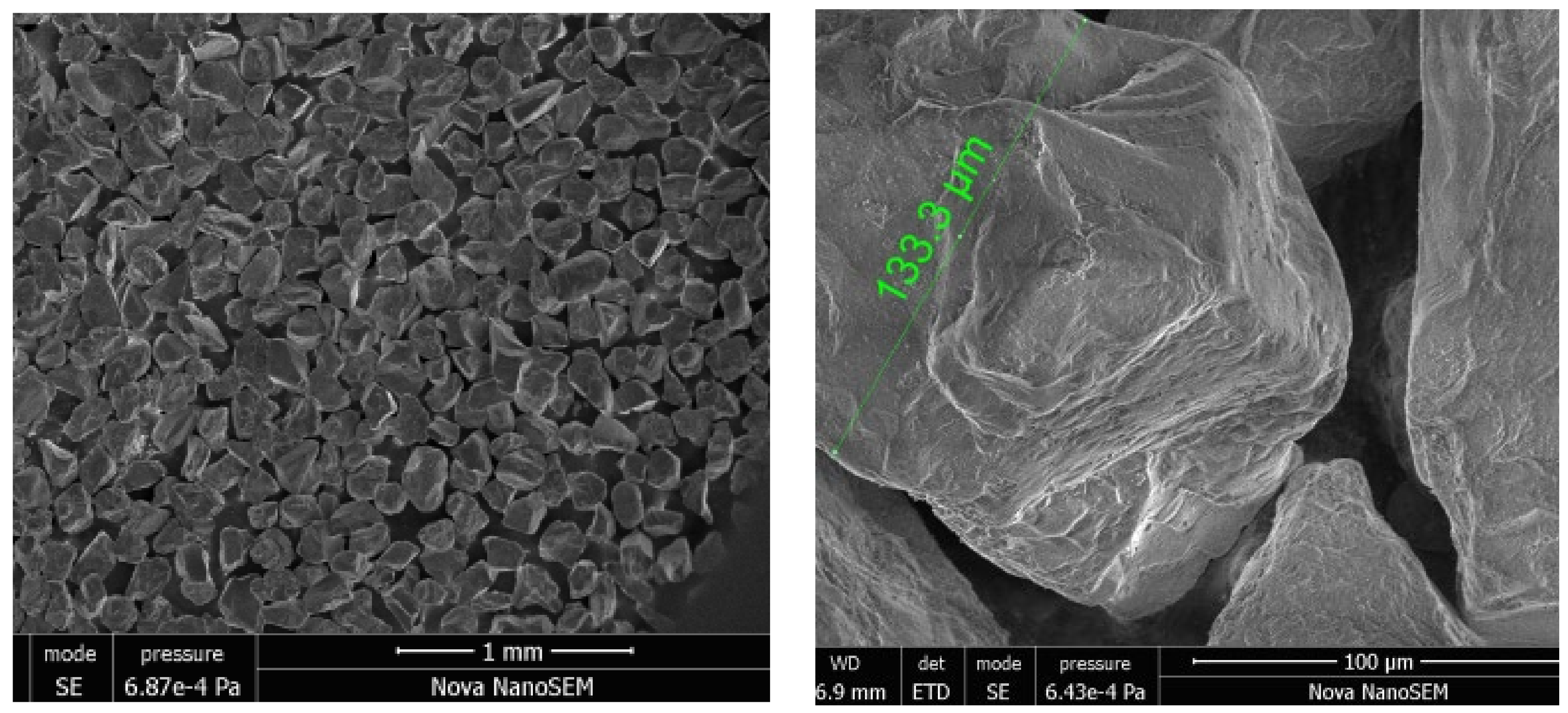
2.1. Test Material

The specimens are constructed using Fujian sand, which is a standard sand that is widely used in China. This material is obtained from the Fujian area of China, which is a river clean sand containing a wide range in grain sizes. Figure 1 shows the particle size distribution of Fujian sand, while only the sand with grain size ranges from 0.1 to 0.25 mm is used to prepare the specimens. The scanning electron microscope images of the sand particles are presented in Figure 2. The particles have rough surfaces and irregular shapes. The physical properties of the Fujian sand are determined in the laboratory, as presented in

Table 1. Physical properties of the Fujian sand.

Soil	Gs	emin	emax	d50 (mm)	d10 (mm)	d60/d10
Fujian sand	2.64	0.69	1.01	0.175	0.115	1.65

.

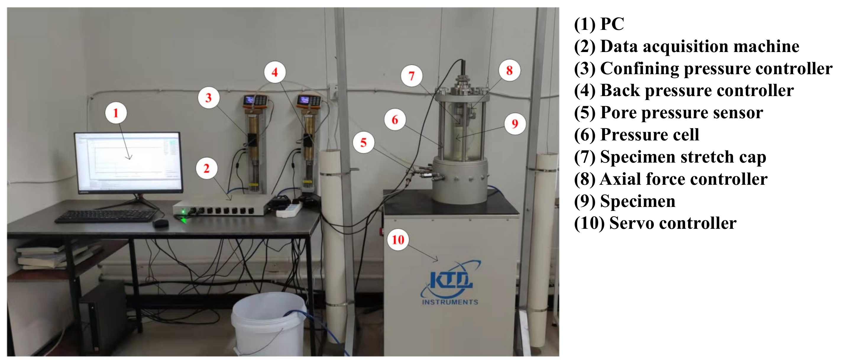
2.2. Test Apparatus, Specimen Preparation, and Testing Procedure

The KTL-DYN8CH cyclic triaxial test apparatus is used in this research (Figure 3). The apparatus consists of an electro-hydraulic servo controller with a double amplitude displacement of 50 mm (±0.035 mm) and an operational frequency range of 0.01–5 Hz. The confining chamber is designed to handle pressure up to 2 MPa. Three pressure transducers are equipped to measure cell pressure, back pressure, pore-water pressure, with the maximum capacity of 2 MPa, and a load transducer to measure the submersible load less than 10 kN. The testing is controlled by a fully automatic dynamic controller unit, which conveys the instructions and records the testing data with the help of the GeoSmart Lab software.

All solid cylinder specimens are 50 mm in diameter and 100 mm in height. According to China standard [36], the specimens are prepared using the dry pluviation method in this study. The oven-dried Fujian sand specimens are prepared in four layers into the membrane-lined split mold with a funnel. A vacuum pressure of 20 kPa is applied before removing the mold to maintain the stability of the sand specimen. Then the confining chamber is installed, and de-aired water is filled, followed by the saturation and consolidation stages. The CO₂ is flushed through each specimen for about 1 h using a confining pressure-assist of about 20 kPa, to accelerate the saturation process. Then, the de-aired water passes through each specimen from the bottom to the top until the air bubble disappears. This process generally takes 30 min, followed by increasing the back pressure and confining pressure step by step. The B value of 0.95 (i.e., complete saturation) is generally obtained when the back pressure is about 300–400 kPa in this study. The specimen is isotropically consolidated to the target effective confining pressure in a loading sequence. Time of confinement is at least 250 min at each pressure during the period of tests.

A series of strain-controlled cyclic triaxial tests are then performed at 1.0 Hz loading frequency, corresponding to the strain level which varies from 10⁻⁴ to 10⁻². Five cycles of cyclic loading are applied during cyclic triaxial tests and the second cycle of loading is used to determine the shear modulus in the present study. The sand specimens are tested at three different relative densities (D_r = 30%, 50%, 70%) and six effective confining pressures (σ_c = 50, 100, 300, 500, 700, 900 kPa).

3. Determination Methods of Shear Modulus

As mentioned above, the shear modulus of Fujian sand is measured according to the hysteresis loop at a given strain amplitude. Thus, this section attempts to introduce briefly the four methods used for determining the shear modulus.

3.1. Hysteresis Loop Method

Assuming the visco-elastic of soil, the dynamic stress, σ_d, and the corresponding dynamic strain, ε_d, can be written as follows [28]:

$$\left\{\begin{array}{c}{\sigma }_{\mathrm{d}}={\sigma }_{\mathrm{a}}sin\omega t\\ {\epsilon }_{\mathrm{d}}={\epsilon }_{\mathrm{a}}sin\left(\omega t-\delta \right)\end{array}\right.$$

(1)

where σ_a, and ε_a are, respectively, the amplitudes of dynamic stress and dynamic strain, ω is the frequency of cyclic loading; δ is the phase lag between strain and stress. As shown in Figure 4a, the hysteresis loop is symmetric at a given strain level. Therefore, the shear modulus is usually expressed as the secant modulus determined by the extreme points on the hysteresis loop. This method is widely utilized in current practice [23], using the following equation:

$$E_{\sec }=\frac{{\sigma }_{\mathrm{d}}}{{\epsilon }_{\mathrm{d}}}=\frac{{\sigma }_{\mathrm{d},\max }-{\sigma }_{\mathrm{d},\min }}{{\epsilon }_{\max }-{\epsilon }_{\min }}$$

(2)

$$G=E_{\sec }/2(1+\mu )$$

(3)

$$\gamma =\left(1+\mu \right)\epsilon$$

(4)

where $\mu$ is the Poisson’s ratio. For the saturated specimen, a value of 0.5 is utilized.

3.2. Arithmetical Average Method

Kumar et al. [29] pointed out that the conventional method assuming a symmetrical hysteresis loop may lead to underestimation or overestimation of the real dynamic shear modulus. To account for the effect of actual strain energy and modulus value in compression, E_sec1, and in tension E_sec2, an averaged secant modulus, E_sec,a, was suggested, as shown in Figure 4b. To the actual representation of asymmetric nature of hysteresis loop, the arithmetical average method defines the scant modulus as follows:

$$E_{\sec ,\mathrm{a}}=\frac{E_{\sec 1}+E_{\sec 2}}{2}$$

(5)

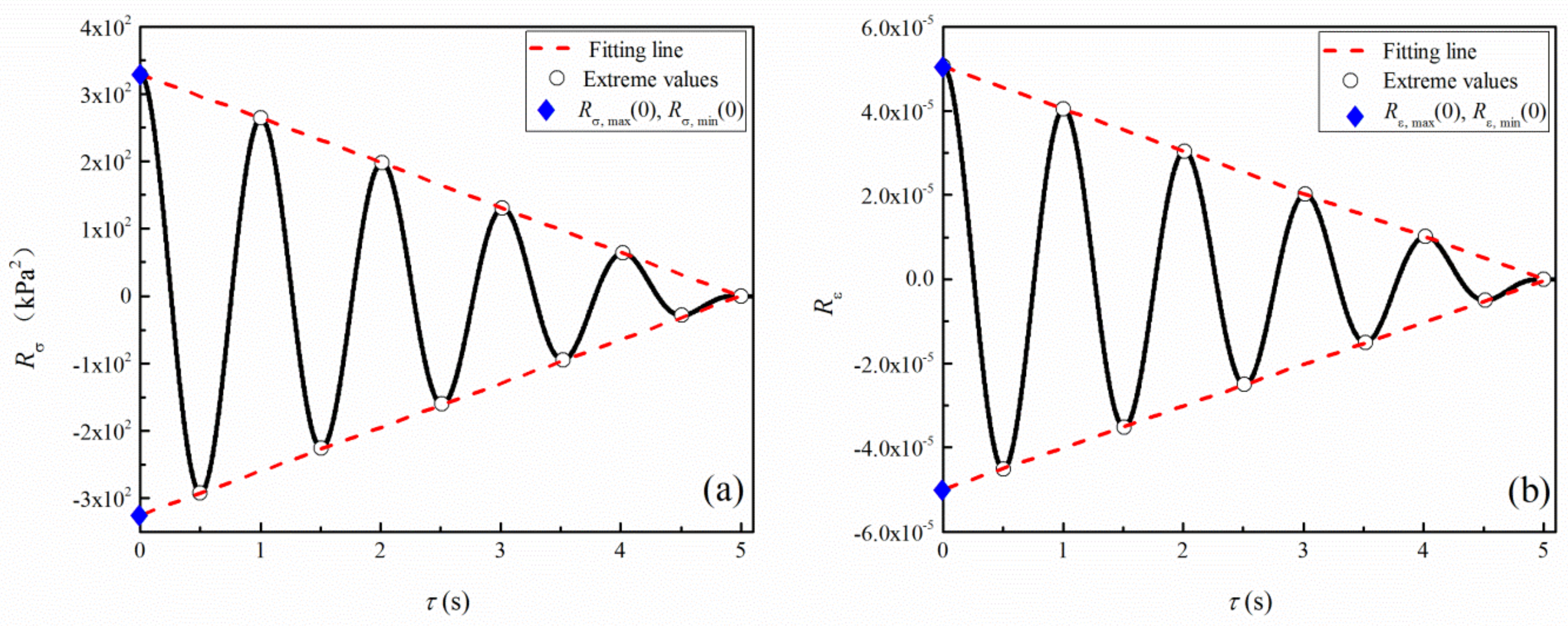
3.3. Autocorrelation Function Method

At small strains, the stress–strain measurements tend to be distorted by ambient noise because of the low signal-to-noise ratios, as well as sensor accuracy. This leads to the presence of the white noise component in the time histories of dynamic strain and dynamic stress. To eliminate these adverse effects, Liang et al. [30] proposed a new method for the calculation of dynamic shear modulus based on the theory of correlation function. The correlation function quantifies the similarity of two waveforms at different times τ. For the waveform x(t) with a time length of t₀, the autocorrelation function R_x(τ) can be written:

$$R_x\left(\tau \right)=\frac{1}{t_0}{{\displaystyle \int }}_0^{t_0}x\left(t\right)x\left(t+\tau \right)dt$$

(6)

Substituting Equation (6) into Equation (1), the autocorrelation function of an ideal stress waveform is:

$$R_{\sigma }\left(\tau \right)=\frac{1}{NT}{{\displaystyle \int }}_0^{NT-\tau }{\sigma }_a^{2}sin\left(wt\right)sin\left(wt+w\tau \right)dt=\frac{{\sigma }_a^2}{2NT\omega }sin\left(w\tau \right)+\frac{\left(NT-\tau \right){\sigma }_a^2}{2NT}cos\left(w\tau \right)$$

(7)

where N and T are the number and period of cyclic loading, respectively. The extreme values of Equation (7) can be determined based on the first-order derivative $\stackrel{•}{R}$_σ(τ). Thus:

$$\left\{\begin{array}{c}{R}_{\mathsf{\sigma },\max }\left(\tau \right)=\frac{NT-\tau }{2NT}{\sigma }_a^2\tau =0,T,\dots NT\\ R_{\sigma ,min}\left(\tau \right)=-\frac{NT-\tau }{2NT}{\sigma }_a^2\tau =0.5T,1.5T,\dots \left(N-0.5\right)T\end{array}\right.$$

(8)

The amplitude of dynamic stress can then be derived at τ = 0:

$${\sigma }_a=\sqrt{R_{\mathsf{\sigma },\max }\left(0\right)-R_{\mathsf{\sigma },\min }\left(0\right)}$$

(9)

Similarly,

$${\mathsf{\epsilon }}_a=\sqrt{R_{\mathsf{\epsilon },\max }{}_{}\left(0\right)-R_{\mathsf{\epsilon },\min }\left(0\right)}$$

(10)

To provide a better understanding of this method, the autocorrelation functions of stress and of strain time histories, including R_σ,max(0), R_σ,min(0), R_ε,max(0), and R_ε,min(0) are illustrated in Figure 5.

3.4. Least Square Method

Shen and Chen [31] presented the advantage of using the least square method to calculate the shear modulus to overcome the influence of the irregularity of the hysteresis loop. The principle behind this method is presented herein. At small strains, the relationship between dynamic stress and dynamic strain at time i, should satisfy Equation (11):

$$E{\epsilon }_{\mathrm{i}}+{\sigma }_0={\sigma }_{\mathrm{i}}$$

(11)

Considering there is n data pairs for the measured stress and strain time histories:

$$E{{\displaystyle \sum }}_{i=1}^n{\epsilon }_{\mathrm{i}}+n{\sigma }_0={{\displaystyle \sum }}_{i=1}^n{\sigma }_{\mathrm{i}}$$

(12)

By multiplying both sides of Equation (11), the strain ε_i:

$$E{\epsilon }_{\mathrm{i}}^2+{\sigma }_0{\epsilon }_{\mathrm{i}}={\sigma }_{\mathrm{i}}{\epsilon }_{\mathrm{i}}$$

(13)

Similarly, summing up the Equation (13) for n data pairs gives:

$$E{{\displaystyle \sum }}_{i=1}^n{\epsilon }_{\mathrm{i}}^2+{\sigma }_0{{\displaystyle \sum }}_{i=1}^n{\epsilon }_{\mathrm{i}}={{\displaystyle \sum }}_{i=1}^n{\sigma }_{\mathrm{i}}{\epsilon }_{\mathrm{i}}$$

(14)

where σ₀ is the initial axial stress, σ_i and ε_i is the axial stress, and the strain at the time i. Combining Equation (12) and Equation (14), the secant modulus E can be calculated from:

$$E=\frac{{{\displaystyle \sum }}_{i=1}^n{\sigma }_{\mathrm{i}}{{\displaystyle \sum }}_{i=1}^n{\epsilon }_{\mathrm{i}}-n{{\displaystyle \sum }}_{i=1}^n{\sigma }_{\mathrm{i}}{\epsilon }_{\mathrm{i}}}{{{\displaystyle \sum }}_{i=1}^n{\epsilon }_{\mathrm{i}}{{\displaystyle \sum }}_{i=1}^n{\epsilon }_{\mathrm{i}}-n{{\displaystyle \sum }}_{i=1}^n{\epsilon }_{\mathrm{i}}^2}$$

(15)

4. Results

The dynamic properties of Fujian sand tested at different relative densities and effective confining pressures, measured by the strain-controlled cyclic triaxial apparatus under isotropic stress conditions in the nonlinear range (10−4~10−2), are presented in this section. The section is divided into two sub-sections, the first one dealing with the G-γ relationship, the second one dealing with the relationship between the normalized shear modulus and the shear strain (G/G_max-γ). In each sub-section, the results of four determination methods are compared and the relative difference of three newly proposed methods (i.e., arithmetical average method, autocorrelation function method, least square method) with the conventional method (i.e., hysteresis loop method) are illustrated.

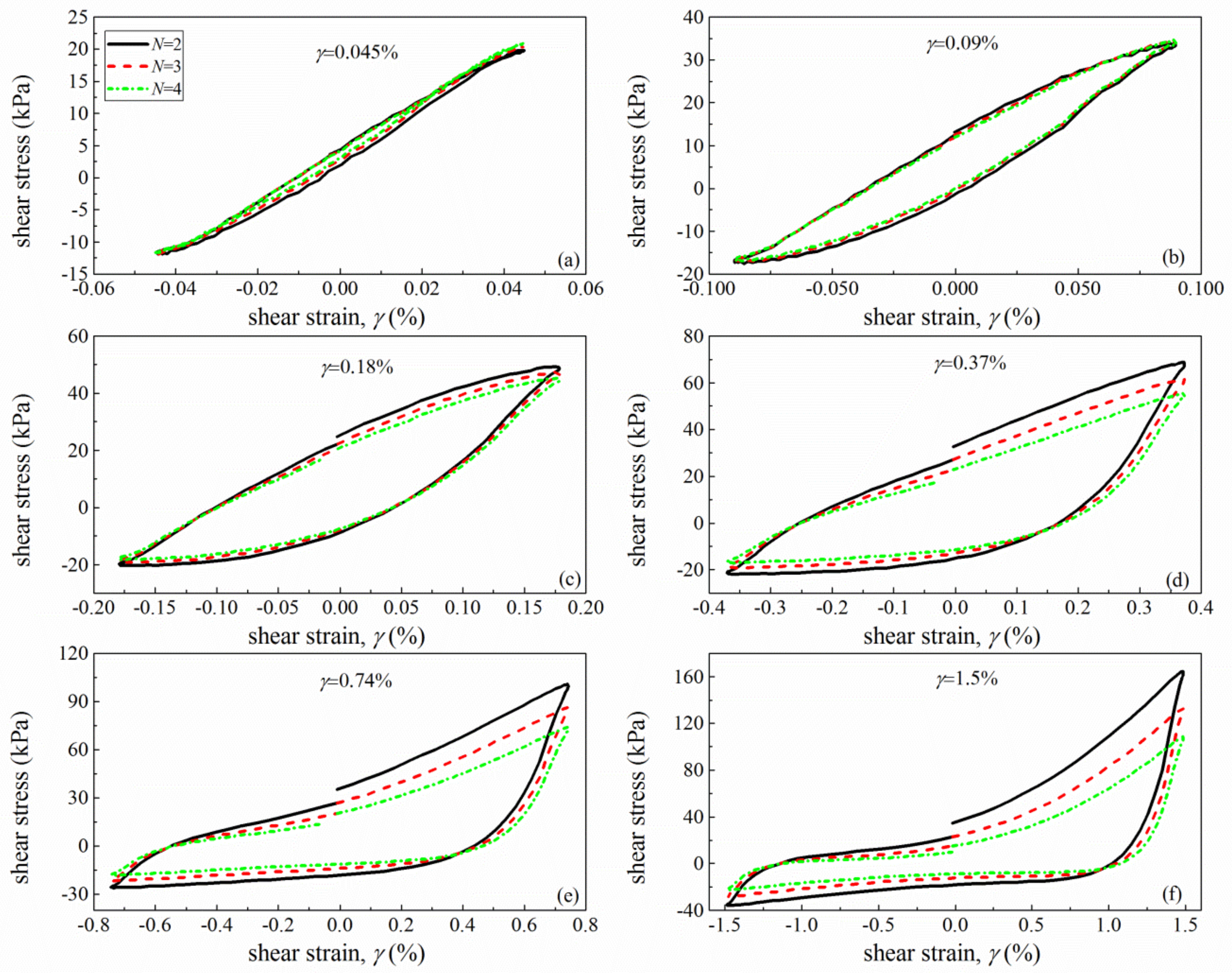
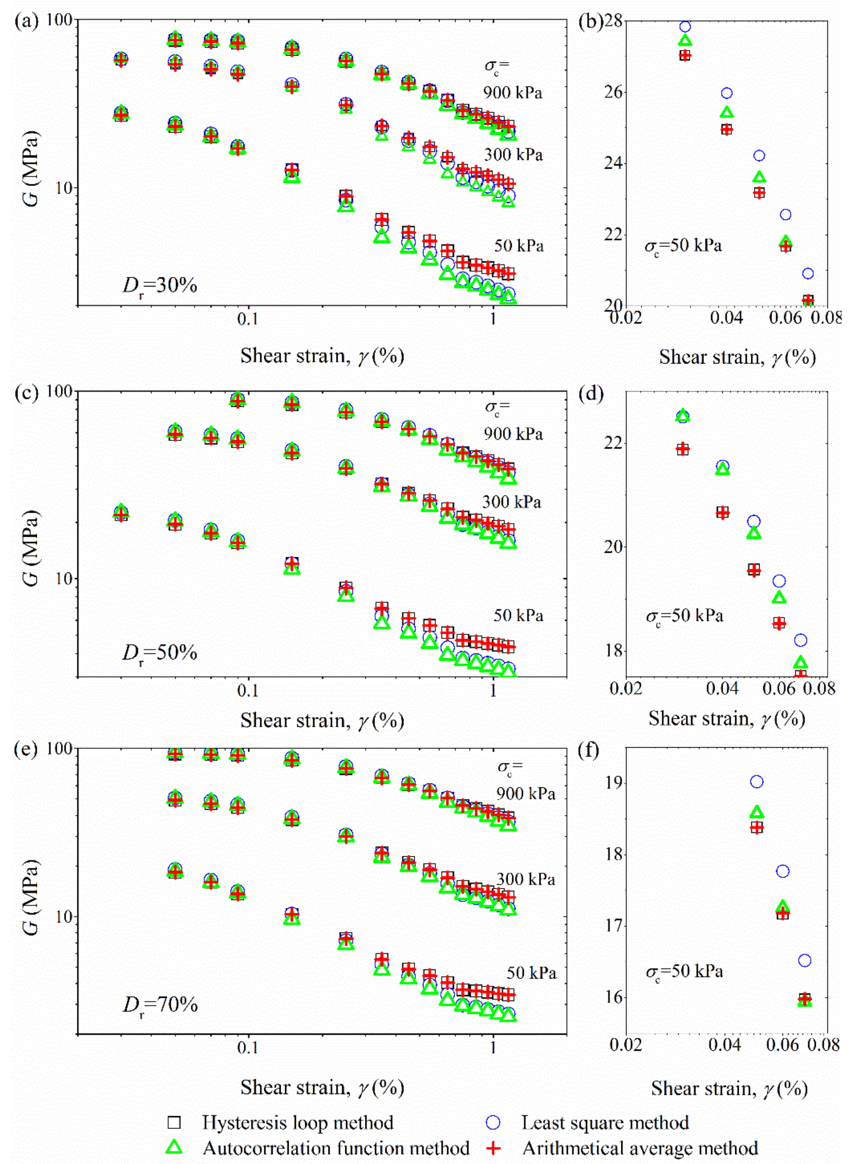
4.1. G~γ Curves

For a given γ amplitude, the hysteresis loops of the specimens subjected to five numbers of loading cyclic (N) are measured with a loading frequency of 1.0 Hz, for D_r = 30, 50, 70% and σ_c = 50, 100, 300, 500, 700, 900 kPa. The value of G can then be calculated from the measured cyclic hysteresis loop. As an example, Figure 6 depicts the representative hysteresis loops (N = 2~4) for increasing γ values in the range of 0.045~1.5% (the specific strain amplitudes are given in the subplots), which corresponds to the D_r = 50%, and σ_c = 100 kPa. As can be observed, the shapes of the stress–strain loops measured are consistent with the expected shape up to a shear strain of 0.74% whereas the hysteresis loop becomes progressively asymmetric with increasing γ. At high strains, the “banana shape” of the hysteresis loop appears. It is often assumed that the “banana shape” is due to the dilation of the test specimen at higher shear strains. This trend is consistent with the findings in the literature [29].

Moreover, it appears that the loading cyclic number N has a pronounced influence on the shape of hysteresis loops with the influence becoming larger as the γ increases. From Figure 6, the shear modulus shows a tendency of decrease with increasing N [7,15,19,34]. In this study, the second cyclic loading and the corresponding hysteresis loop has been utilized for determining the value of G. The influence of the hysteresis loop selection on the measured G will be discussed in the next section.

Figure 7 presents the variation of shear modulus with changes in shear strain for three different relative densities (D_r = 30, 50, 70%) and three representative confining pressures (σ_c = 50, 300, 900 kPa). Figure 7a,c,e present the results for the variation of shear modulus in the entire shear strain range while the variations of shear modulus at medium shear strains (10⁻⁴~10⁻³), corresponding to σ_c = 50 kPa are shown in Figure 7b,d,f. As expected, the shear modulus is strongly dependent on the shear strain amplitude and the effective confining pressure. The increase in the confining pressure leads to an increase in the shear modulus while the shear modulus decreases as the shear strain increases. Concerning the influence of determination methods, four methods capture similar trends. More specifically, at medium shear strain (10⁻⁴~10⁻³), the variation of shear modulus is not significant. The least square method and the autocorrelation function method predict similar G values, both of them are slightly larger than the ones of the conventional method (i.e., hysteresis loop method).

At higher shear strain (10⁻³–10⁻²), an opposite trend is observed. Both the autocorrelation function method and least square method predict the smaller G in comparison to the hysteresis loop method, with the minimum value appearing for the autocorrelation function method. It appears that the difference in shear modulus at higher shear strain is more obvious for lower σ_c. In addition, the arithmetical average method and hysteresis loop method match very well for all the strain amplitudes tested here. It indicates that the arithmetical average method proposed by Kumar et al. [29] does not improve the accuracy of the hysteresis loop method on the estimation of shear modulus. This observation agrees well with the findings in Kumar et al. [29]. In their study, the comparison of two methods was conducted in the strain range of around 4 × 10⁻⁴~2 × 10⁻², corresponding to D_r = 30%, and σ_c = 100 kPa.

The percentage changes (δ) in the shear modulus are illustrated in Figure 8. The δ is defined as the relative difference of the shear modulus between the other three methods and the hysteresis loop method. The results of the arithmetical average method are not plotted since negligible differences (10⁻³ in general) are observed for all the cases considered.

For D_r = 30% and σ_c = 50 kPa, it appears that the relative difference for the least square method in the medium strain range (10⁻⁴~10⁻³) is a little larger than that obtained by the autocorrelation function method. Compared to the hysteresis loop method, a slight overestimation of about 5% is observed. However, the difference may not be particularly significant relative to the difference observed at higher strains. With the increase of γ, the relative differences for the two methods increase sharply. At γ equals to 1%, a decrease of the shear modulus of about 28% for the autocorrelation function method and about 23% for the least square method is captured, respectively. In addition, the curves of relative difference gradually become flattered with the σ_c with increases from 50 to 900 kPa. The relative difference is decreased to about 10% for the two methods at γ = 1% for σ_c = 900 kPa. A wider strain range of shear modulus overestimation, to some extent, appears for the increased σ_c. For example, the threshold shear strain at which δ = 0 varies from about 0.1% at σ_c = 50 kPa to about 0.5% at σ_c = 900 kPa. For D_r = 50% and 70%, similar trends are observed. However, the relative difference of shear modulus is found to be a little smaller than that at D_r = 30%.

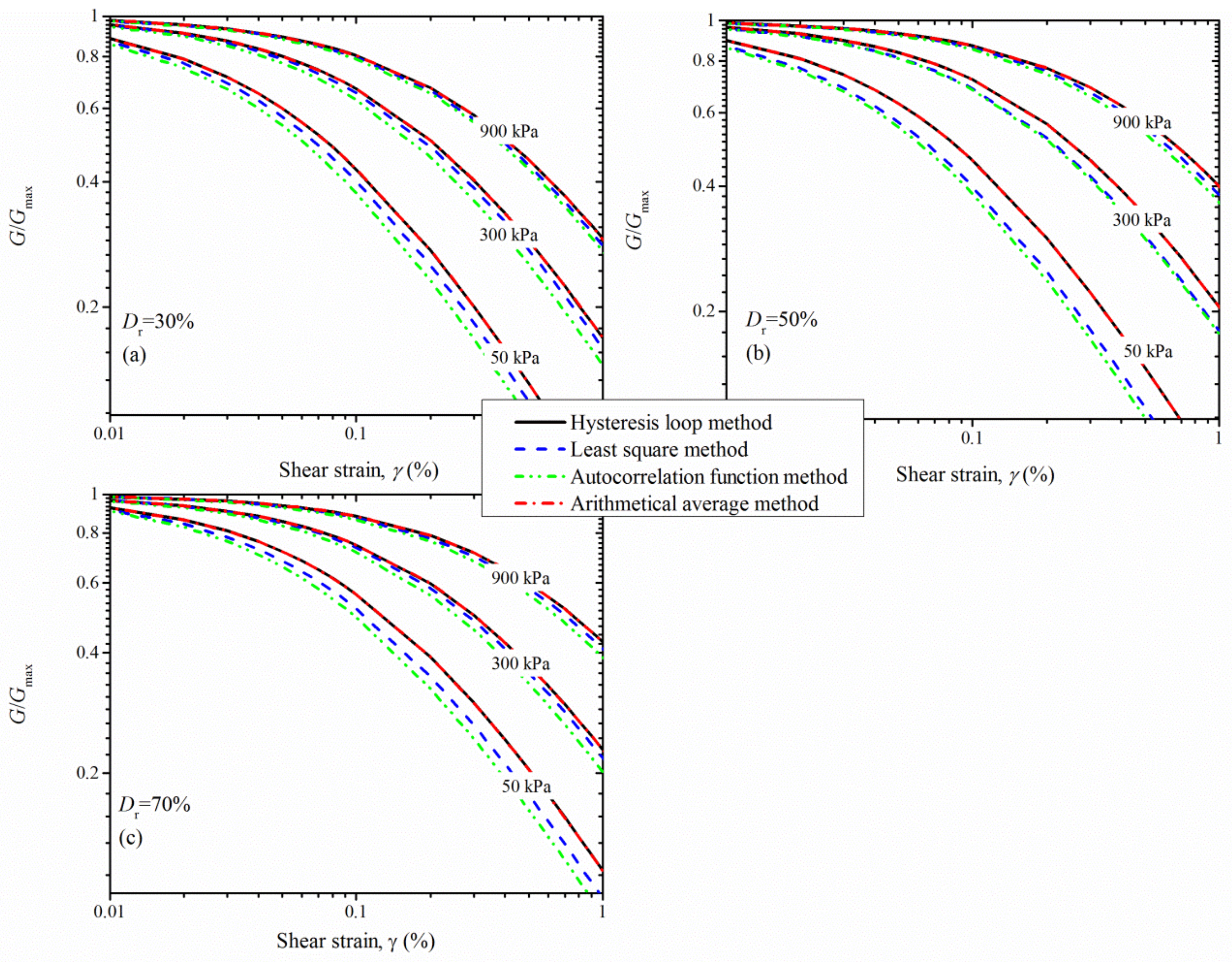
4.2. G/G_max~γ Curves

The normalized modulus reduction curve is used to represent the reduction of shear modulus with increasing shear strain, abbreviated as G/G_max. In CT tests, there are two methods for finding G_max. The first one is the extrapolation of the experimental data in the strain range of around 10⁻⁴ to 10⁻², with the help of an empirical equation. The hyperbolic model proposed by Hardin and Drnedeli [37] is used in this study. Equations (2) and (3) can be rewritten as follows:

$$G=\frac{1}{a+b\gamma }$$

(16)

where a and b are the fitting parameters, respectively. In general, the shear modulus at γ = 1 × 10⁻⁶ is assumed as the small strain shear modulus G_max. This assumption is also utilized here.

Revisiting the Equation (16), it can also be rewritten as follows:

$$\frac{1}{G}=a+b\gamma$$

(17)

Assuming γ = 0, G_max can thus be calculated using the following equation:

$$G_{max}=\frac{1}{a}$$

(18)

For the same set of measured data in CT tests, G_max can be found using Equations (16) and (18), respectively. As an example, Figure 9 schematically shows two methods to determine the G_max, corresponding to G-γ curves for σ_c = 300 kPa and D_r = 70%. However, it should be noted that the values of a and b of Equations (16) and (17) show minor difference, since the hyperbolic and linear models are used to fit the measured data, respectively. Different coefficients of determination are also observed. Furthermore, the G_max is calculated based on 1/a assuming γ = 0, rather than γ = 10⁻⁶. These two reasons which result in the calculated G_max values show certain difference.

A systematic comparison between two estimation methods of G_max is carried out, and some discrepancies are observed in both the G_max and the corresponding G/G_max curves. This issue is discussed in detail in Section 5.1. The representative G/G_max~γ curves for three relative densities (D_r = 30, 50, 70%) and three effective confining pressures (σ_c = 50, 300, 900 kPa) are presented in Figure 10.

These plots show that as the shear strain increases, the shear modulus decreases once a threshold strain is exceeded. The threshold strain ranges from 0.001% to 0.01% showing an increase in the threshold strain with increasing effective confining pressure. As noted in Figure 10, the normalized shear modulus curves determined by the hysteresis loop method and the arithmetical average method are almost identical. The G/G_max-γ curves measured by the other two methods (i.e., least square method and autocorrelation function method) shift on the downsides. The increased non-linearity can be attributed to the larger shear modulus measured at the medium strain while the smaller one at the higher strain leads to steeper shear modulus reduction curves (Figure 7). In addition, it can be observed that the G/G_max curve varies in a narrow band for the high effective confining pressure (i.e., σ_c = 900 kPa), indicating a decreased effect of determination methods.

Available data of reference shear strain γ_r, corresponding to G/G_max = 0.5, are reported in Figure 11 for different relative densities and effective confining pressures. A trend between γ_r and σ_c, D_r can be recognized. As σ_c or D_r increases, γ_r also tends to increase linearly. This is consistent with the findings in the literature [5,26,38]. It should be emphasized that a reduction in γ_r is observed for the case of σ_c = 900 kPa and D_r = 30%. This is probably caused by the breakage of sand particles during the testing, and more fine contents are found at the end of testing. The influence of determination methods is consistent for all the σ_c and D_r cases. In particular, the γ_r calculated by the autocorrelation function method is lower compared to the other methods while the hysteresis loop method and arithmetical average method capture almost the same γ_r and, on the top of that, of the least square method.

The percentage changes (δ) in the normalized shear modulus are reported in Figure 12. The results of the least square method and autocorrelation function method are compared against ones of the hysteresis loop method. The results of shear strain less than 0.02% are not presented since the relatively small percentage changes are observed in this strain range.

For D_r = 30% and σ_c = 50 kPa, the relative difference for the two determination methods increases with increasing shear strain, with the maximum δ of about 20% for the autocorrelation function method and about 10% for the least square method. As σ_c increases, the relative difference appears to decrease. This follows the same trend observed for the G shown in Figure 8. For σ_c = 900 kPa, the percentage changes at γ = 1% of two determination methods decrease to around 5%. In addition, similar trends are captured for the cases of D_r = 50% and 70%. Compared to σ_c, D_r is found to be the second factor that affects the uncertainties introduced by different determination methods.

5. Discussion

The previous discussion illustrates the significant difference in G and G/G_max curves caused by four determination methods, corresponding to the second hysteresis loop and G_max = G_γ=10⁻⁶. This section attempts to discuss the definition of G_max and the choice of cycle number on the results. In particular, the limitation of the autocorrelation function method for computing the shear modulus found during the course of the present study is presented.

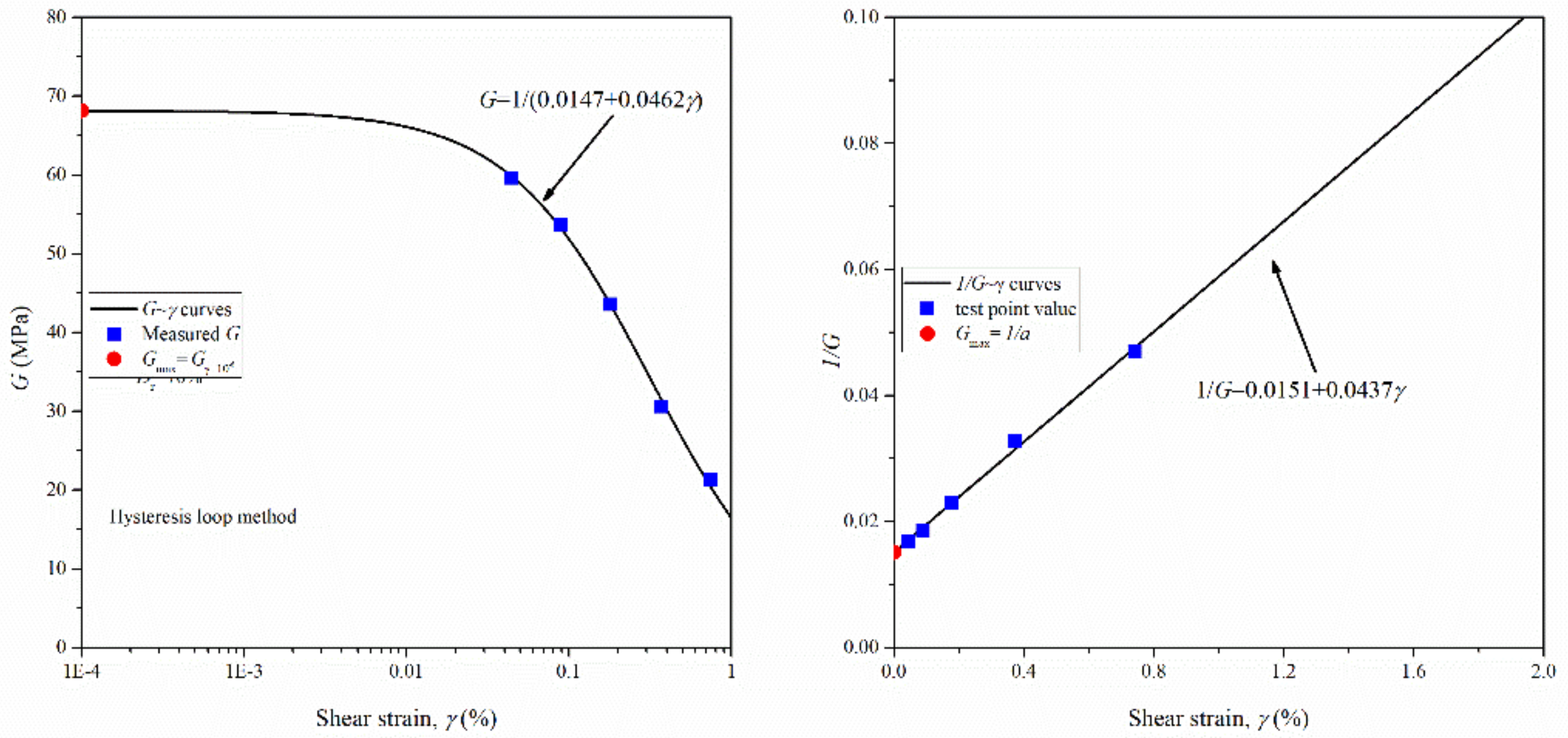
5.1. Definition of G_max

In the laboratory, the small strain shear modulus G_max is more practical to be determined using the bender element or resonant column tests [12,39,40,41]. In the present study, it is determined by the extrapolation of the experimental data in the strain range of around 10⁻⁴ to 10⁻², with the help of an empirical equation [37]. As mentioned above, there are two definitions of the small strain shear modulus G_max: G_γ=10⁻⁶ and 1/a. Both of the two definitions have been utilized to estimate approximately the small strain shear modulus in the literature. Therefore, the uncertainties of G/G_max associated with the definitions of G_max from G_γ=10⁻⁶ and 1/a may be different when compared to each other. In this section, a systematic comparison between two definitions of G_max is carried out, corresponding to D_r = 70%, σ_c = 50~900 kPa.

Figure 13 shows the comparison of the calculated G_max for the four G determination methods. As can be observed, the G_max calculated by 1/a is larger than that of G_γ=10⁻⁶. For instance, the autocorrelation function method predicts the maximum G_max, with a relative difference of more than 20% for σ_c = 900 kPa. The hysteresis loop method and arithmetical average method compute the same value of G_max, but slightly smaller than that of the least square method, with the relative difference generally around 10%. Nevertheless, two definitions of G_max capture the same trend in terms of the influence of four determination methods. This phenomenon is in agreement with the findings shown in Figure 8.

The previous discussion has highlighted the effects of different definitions on G_max. The discrepancy observed in the G_max will influence the corresponding G/G_max curves. Figure 14 presents the comparison of the normalized shear modulus curves for different determination methods. The figure clearly shows the relationship between the G_max and the corresponding G/G_max curves for various effective confining pressures and determination methods. In fact, it can be observed that a slope with the G_max that has been determined by the 1/a will have a steeper gradient than with one that has been determined by the G_γ=10⁻⁶. This phenomenon is valid for various determination methods considered in this study. Additionally, for high σ_c (i.e., 500~900 kPa), the G/G_max curves normalized by G_max = 1/a varies generally in a narrow band, and are almost identical for the autocorrelation function method in particular. Oppositely, the confining effect (i.e., the higher σ_c, the larger G/G_max) seems to be well captured when G_max is estimated at γ = 10⁻⁶.

The previous discussion has clearly illustrated that the G/G_max curves obtained using the autocorrelation function method and the least square method are generally low when G is normalized by G_γ=10⁻⁶. This phenomenon is also observed when G_max is calculated using 1/a, as shown in Figure 15a. As noted in Figure 15a, for the same G determination method, a significant difference in the G/G_max appears for two definitions of G_max. For instance, when G_max is calculated by 1/a, the G/G_max determined by the autocorrelation function method is typically 30~40% lower than that of the hysteresis loop method in the strain range of 10⁻³~10⁻² at σ_c = 50 kPa (Figure 15b) while the percentage change is 20~25% for the G_γ=10⁻⁶ case, as depicted in Figure 12. From Figure 15b, the decreased relative difference with increasing effective confining pressure can be observed. Additionally, the relative difference will further increase when both the uncertainties associated with the G determination methods and definitions of G_max are considered. For instance, for σ_c = 900 kPa, the relative difference of G/G_max between the autocorrelation function method with G_max = 1/a (i.e., green dash line, Figure 15a) and the hysteresis loop method with G_max = G_γ=10⁻⁶ (i.e., black solid line, Figure 15a) can be up to around 50% at γ = 10⁻².

The discussion presented in this section further highlights that the adverse influence of the random choice of determination methods for both G and G_max on the G/G_max. Different G/G_max results are obtained and some of them differ significantly. Therefore, a unified determination method that accurately represents the irregularity of the hysteresis loop at large strains is warranted. Thus, the uncertainties associated with the G/G_max measurements, to some extent, can be reduced. This would be highly beneficial for engineering and practical because more accurate empirical models could be developed if the uncertainties in G/G_max are substantially eliminated [2,5,6,23,38].

5.2. Limitation of the Autocorrelation Function Method

As presented in Section 3.3, the principle behind the autocorrelation function method is to quantify the similarity of two waveforms at different times τ, using correlation functions. It can be observed that stress or strain time histories are highly correlated at different τ, when the applied strain amplitude is relatively small since the ignorable influence of the number of cyclic loading N, as noted in Figure 6a,b. However, at large strains, the similarity gradually diminishes with increasing N, the stress time histories in particular. Although the previous study used the second cycle to calculate the G for the other three determination methods, it is the entire stress and strain time histories that are used for the autocorrelation function method, rather than a single loading cycle (i.e., one cycle is impossible to compute the autocorrelation function).

Therefore, the aforementioned means that the autocorrelation function method discards the influence of N on both G and G/G_max. As an example, Figure 16 compares the G/G_max results of N = 2, 3, and 4 for various determination methods, corresponding to D_r = 30% and σ_c = 50 kPa. It can be observed that the autocorrelation function method predicts identical G/G_max curves, and illustrates the average result of the five hysteresis loops. Both the hysteresis loop method and the least square method indicate an increased non-linearity for high N. This leads to the G/G_max curves of these two methods which are on the top for N = 2 whereas these two curves move to the downsides for N = 4. Additionally, Figure 16 further demonstrates the influence of N on the uncertainty quantification of determination methods, particularly in the large strain range. For instance, the percentage change of the least square method tends to decrease with increasing N, with a maximum δ of around 5% for N = 4.

6. Conclusions

In this study, a comparison of the shear modulus measurements in cyclic triaxial tests using various determination methods is performed. The sand specimens, prepared with three relative densities, are tested at medium to large strains and from low to high confining pressures. Four methods, namely: hysteresis loop method, least square method, autocorrelation function method, and arithmetical average method, are adopted to determine the shear modulus from the second hysteresis loop. The uncertainty associated with the determination method is quantified. Based on the comparative study performed, the following conclusions can be drawn:

(1)

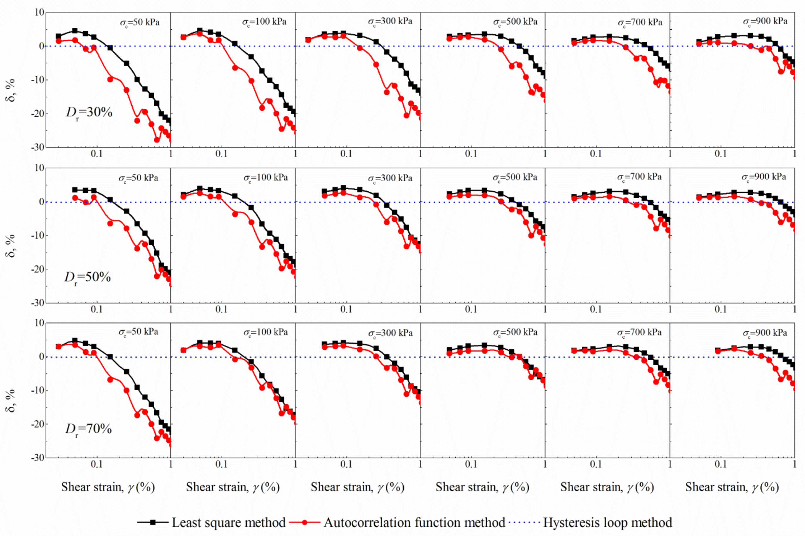
The hysteresis loop is generally symmetrical and it becomes progressively asymmetric with increasing γ. In addition, the loading cyclic number N has a pronounced influence on the hysteresis loops with the influence becoming larger as γ increases. Both the G and G/G_max show a tendency of decrease with increasing N.

(2)

The G and G/G_max are strongly dependent on amplitudes of γ and σ_c. The increase in σ_c leads to an increase in the G and G/G_max whereas the G decreases as γ increases. At medium shear strains (10−4~10−3), the variation in G and G/G_max is not significant, with a percentage change generally less than 5%. However, the difference increases with decreasing σ_c or increasing γ, with the maximum percentage change of around 30% at σ_c = 50 kPa.

(3)

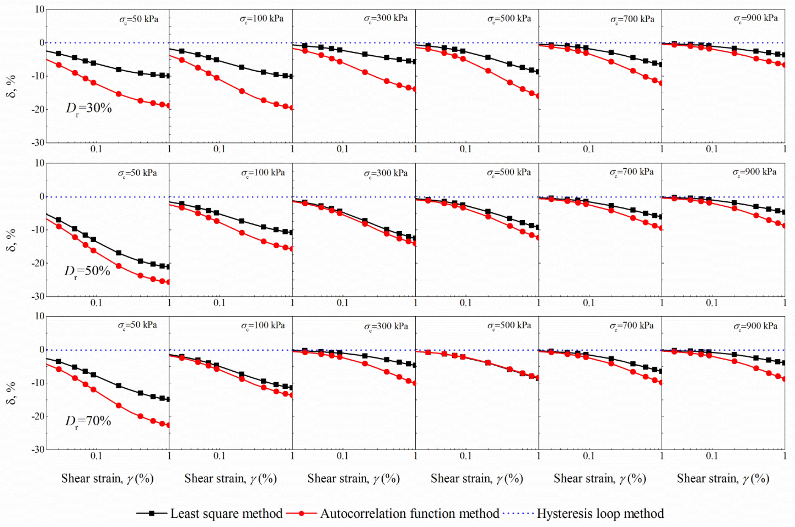
The arithmetical average method predicts almost identical results with the hysteresis loop method. Nevertheless, the larger G estimated at medium strains and the smaller G estimated at large strains for the autocorrelation function method, and least square method results in a steeper gradient of the G/G_max curve. This thus corresponds to a smaller reference strain for these two methods.

(4)

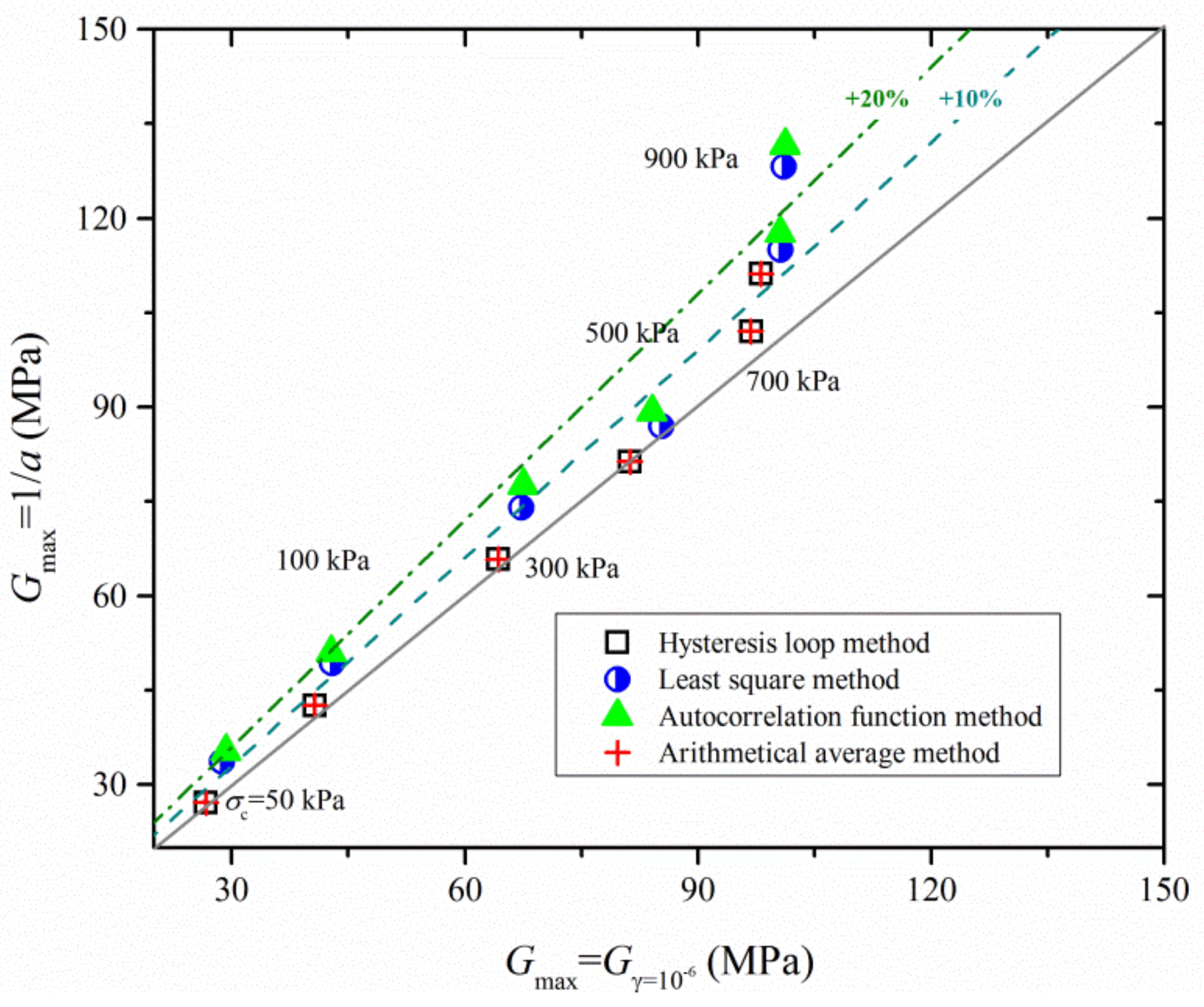
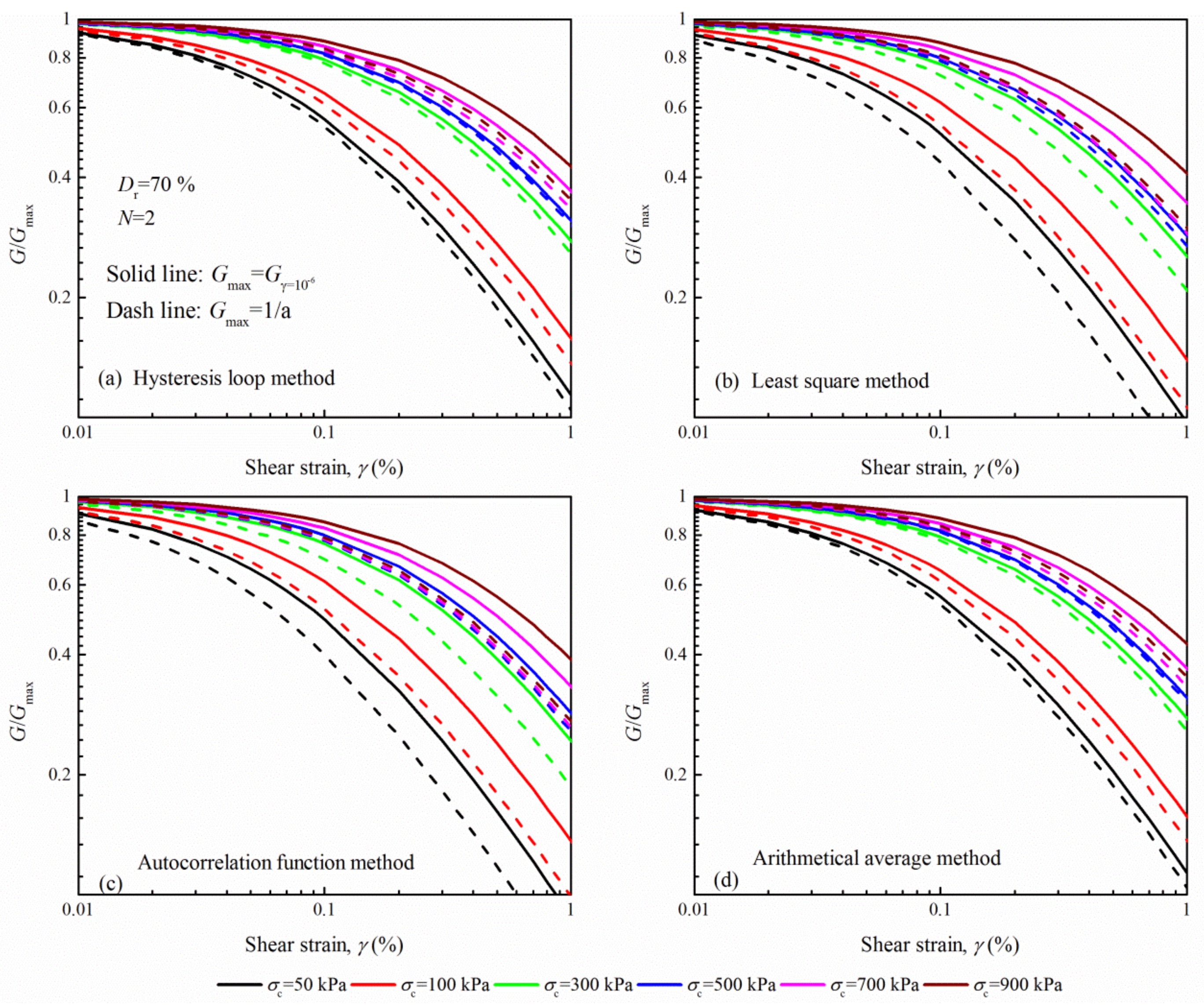
Concerning the definitions of G_max, a relatively large G_max is calculated by 1/a, leading to an increased nonlinearity of G/G_max. The G/G_max determined by the autocorrelation function method is typically 30~40% lower than that of the hysteresis loop method in the strain range of 10−3~10−2 at σ_c = 50 kPa while the percentage change is slightly small (i.e., 20~25%) for the G_γ=10−6 case.

(5)

The autocorrelation function method has no capacity of capturing the dependency of G and G/G_max on N. Both the hysteresis loop method and the least square method indicate an increased nonlinearity for high N. The comparison further demonstrates the influence of N on the uncertainty quantification of determination methods, particularly for large strains.

References

- Ovando-Shelley, E.; Ossa, A.; Romo, M.P. The sinking of Mexico City: Its effects on soil properties and seismic response. Soil. Dyn. Earthq. Eng. 2007, 27, 333–343. [Google Scholar] [CrossRef]
- Seed, H.B.; Wong, R.T.; Idriss, I.M.; Tokimatsu, K. Moduli and damping factors for dynamic analyses of cohesionless soils. J. Geotech. Geoenviron. Eng. 1986, 112, 1016–1032. [Google Scholar] [CrossRef]
- Tika, T.H.; Kallioglou, P.; Koninis, G.; Michaelidis, P.; Efthimiou, M.; Pitilakis, K. Dynamic properties of cemented soils from Cyprus. Bull. Eng. Geol. Environ. 2010, 69, 295–307. [Google Scholar] [CrossRef]
- Tunar-Özcan, R.; Ulusay, R.; Işık, N.S. Assessment of dynamic site response of the peat deposits at an industrial site (Turkey) and comparison with some seismic design codes. Bull. Eng. Geol. Environ. 2019, 78, 2215–2235. [Google Scholar] [CrossRef]
- Darendeli, M.B. Development of a New Family of Normalized Modulus Reduction and Material Damping Curves. Ph.D. Thesis, The University of Texas at Austin, Austin, TX, USA, 2001. [Google Scholar]
- EPRI. Modeling of Dynamic Soil Properties; Electric Power Research Institute: Palo Alto, CA, USA, 1993. [Google Scholar]
- Sun, J.I.; Golesorki, R.; Seed, H.B. Dynamic Moduli and Damping Ratios for Cohesive Soils; Report No. EERC 88-15; Earthquake Engineering Research Center, University of California: Berkeley, CA, USA, 1988. [Google Scholar]
- Hara, A.; Kiyota, Y. Dynamic Shear Test of Soils for Seismic Analyses. In Proceedings of the Ninth International Conference on Soil Mechanics and Foundation Engineering, Tokyo, Japan, 11–15 July 1977. [Google Scholar]
- Isenhower, W.M. Torsional Simple Shear/Resonant Column Properties of San Francisco Bay Mud. Master’s Thesis, The University of Texas at Austin, Austin, TX, USA, 1979. [Google Scholar]
- Kokusho, T. Cyclic triaxial test of dynamic soil properties for wide strain range. Soils Found. 1980, 20, 45–60. [Google Scholar] [CrossRef]
- Doroudian, M.; Vucetic, M. A direct simple shear device for measuring small-strain behavior. Geotech. Test. J. 1995, 18, 69–85. [Google Scholar]
- Menq, F.Y. Dynamic Properties of Sandy and Gravelly Soils. Ph.D. Thesis, The University of Texas at Austin, Austin, TX, USA, 2003. [Google Scholar]
- Seed, H.B.; Idriss, I.M. Soil Moduli and Damping Factors for Dynamic Analysis. Report No. EERC 70-10; Earthquake Engineering Research Center, University of California: Berkeley, CA, USA, 1970. [Google Scholar]
- Bayat, M.; Ghalandarzadeh, A. Modified models for predicting dynamic properties of granular soil under anisotropic consolidation. Int. J. Geomech. 2020, 20, 04019197. [Google Scholar] [CrossRef]
- Chen, G.X.; Zhao, D.F.; Chen, W.Y.; Juang, C.H. Excess pore-water pressure generation in cyclic undrained testing. J. Geotech. Geoenviron. Eng. 2019, 145, 04019022. [Google Scholar] [CrossRef]
- Chen, H.; Jiang, Y.L.; Niu, C.C.; Leng, G.J.; Tian, G.L. Dynamic characteristics of saturated loess under different confining pressures: A microscopic analysis. Bull. Eng. Geol. Environ. 2019, 78, 931–944. [Google Scholar] [CrossRef]
- Bocheńska, M.; Bujko, M.; Dyka, I.; Srokosz, P.; Ossowski, R. Effect of Chitosan Solution on Low-Cohesive Soil’s Shear Modulus G Determined through Resonant Column and Torsional Shearing Tests. Appl. Sci. 2022, 12, 5332. [Google Scholar] [CrossRef]
- Chen, H.; Li, H.; Fu, R.; Yuan, X.Q. Dynamic behaviour and damage characteristics of loess in Xinyang, China. Bull. Eng. Geol. Environ. 2020, 79, 2285–2297. [Google Scholar] [CrossRef]
- Cherian, A.C.; Kumar, J. Effects of vibration cycles on shear modulus and damping of sand using resonant column tests. J. Geotech. Geoenviron. Eng. 2016, 142, 06016015. [Google Scholar] [CrossRef]
- Li, J.; Cui, J.; Shan, Y.; Li, Y.; Ju, B. Dynamic Shear Modulus and Damping Ratio of Sand–Rubber Mixtures under Large Strain Range. Materials 2020, 13, 4017. [Google Scholar] [CrossRef] [PubMed]
- Liang, F.; Zhang, Z.; Wang, C.; Gu, X.; Lin, Y.; Yang, W. Experimental Study on Stiffness Degradation and Liquefaction Characteristics of Marine Sand in the East Nan-Ao Area in Guangdong Province, China. J. Mar. Sci. Eng. 2021, 9, 638. [Google Scholar] [CrossRef]
- Zhang, P.; Ding, S.; Fei, K. Research on Shear Behavior of Sand–Structure Interface Based on Monotonic and Cyclic Tests. Appl. Sci. 2021, 11, 11837. [Google Scholar] [CrossRef]
- Ciancimino, A.; Lanzo, G.; Alleanza, G.A.; Amoroso, S.; Bardotti, R.; Biondi, G. Dynamic characterization of fine-grained soils in Central Italy by laboratory testing. Bull. Earthq. Eng. 2020, 18, 5503–5531. [Google Scholar] [CrossRef]
- Ahn, S.; Ryou, J.-E.; Ahn, K.; Lee, C.; Lee, J.-D.; Jung, J. Evaluation of Dynamic Properties of Sodium-Alginate-Reinforced Soil Using A Resonant-Column Test. Materials 2021, 14, 2743. [Google Scholar] [CrossRef] [PubMed]
- Ling, X.Z.; Zhang, F.; Li, Q.L.; An, L.S.; Wang, J.H. Dynamic shear modulus and damping ratio of frozen compacted sand subjected to freeze-thaw cycle under multi-stage cyclic loading. Soil. Dyn. Earthq. Eng. 2015, 76, 111–121. [Google Scholar] [CrossRef]
- Zhou, W.; Chen, Y.; Ma, G.; Yang, L.; Chang, X. A modified dynamic shear modulus model for rockfill materials under a wide range of shear strain amplitudes. Soil. Dyn. Earthq. Eng. 2017, 92, 229–238. [Google Scholar] [CrossRef]
- Bedr, S.; Mezouar, N.; Verrucci, L.; Lanzo, G. Investigation on shear modulus and damping ratio of Algiers marls under cyclic and dynamic loading conditions. Bull. Eng. Geol. Environ. 2019, 78, 2473–2493. [Google Scholar] [CrossRef]
- Kramer, S.L. Geotechnical Earthquake Engineering; Prentice Hall: Upper Saddle River, NJ, USA, 1996. [Google Scholar]
- Kumar, S.S.; Krishna, A.M.; Dey, A. Evaluation of dynamic properties of sandy soil at high cyclic strains. Soil. Dyn. Earthq. Eng. 2017, 99, 157–167. [Google Scholar] [CrossRef]
- Liang, K.; Chen, G.X.; He, Y.; Liu, J.R. An new method for calculation of dynamic modulus and damping ratio based on theory of correlation function. Rock. Soil. Mech. 2019, 40, 1368–1376. (In Chinese) [Google Scholar]
- Shen, J.R.; Chen, S.L. Method for dynamic modulus based on least square and modified Kumar methods. Chin. J. Geotech. Eng. 2020, 42, 183–187. (In Chinese) [Google Scholar]
- Cheng, K.; Zhang, J.; Miao, Y.; Ruan, B.; Peng, T. The effect of plastic fines on the shear modulus and damping ratio of silty sands. Bull. Eng. Geol. Environ. 2019, 78, 5865–5876. [Google Scholar] [CrossRef]
- Fathi, H.; Jamshidi Chenari, R.; Vafaeian, M. Large scale direct shear experiments to study monotonic and cyclic behavior of sand treated by polyethylene terephthalate strips. Int. J. Civ. Eng. 2021, 19, 533–548. [Google Scholar] [CrossRef]
- Liu, H.X.; Gao, K.F.; Zhu, X. Experimental study on dynamic fatigue properties of dolomite samples under triaxial multilevel cyclic loading. Bull. Eng. Geol. Environ. 2021, 80, 551–565. [Google Scholar] [CrossRef]
- Liu, X.; Li, S.; Sun, L.Q. The study of dynamic properties of carbonate sand through a laboratory database. Bull. Eng. Geol. Environ. 2021, 79, 3843–3855. [Google Scholar] [CrossRef]
- GB/T 50123-2019; Standard for Soil Test Method. China Planning Express: Beijing, China, 2019.
- Hardin, B.O.; Drnevich, V.P. Shear modulus and damping in soils: Design equations and curves. J. Soil. Mech. Found. Div. 1972, 98, 667–692. [Google Scholar] [CrossRef]
- Ishibashi, I.; Zhang, X. Unified dynamic shear moduli and damping ratios of sand and clay. Soils Found. 1993, 33, 182–191. [Google Scholar] [CrossRef]
- Huang, X.; Cai, X.G.; Bo, J.S.; Li, S.H.; Qi, W.H. Experimental study of the influence of gradation on the dynamic properties of centerline tailings sand. Soil Dyn. Earthq. Eng. 2021, 151, 106993. [Google Scholar] [CrossRef]
- Senetakis, K.; Payan, M. Small strain damping ratio of sands and silty sands subjected to flexural and torsional resonant column excitation. Soil. Dyn. Earth. Eng. 2018, 114, 448–459. [Google Scholar] [CrossRef]
- Wichtmann, T.; Triantafyllidis, T. Influence of the grain-size distribution curve of quartz sand on the small strain shear modulus Gmax. J. Geotech. Geoenviron. Eng. 2009, 135, 1404–1418. [Google Scholar] [CrossRef]