Abstract
Oil sheen on the water surface can indicate a source of hydrocarbon in underlying subaquatic sediments. Here, we develop and test the accuracy of an algorithm for automated real-time visual monitoring of the water surface for detecting oil sheen. This detection system is part of an automated oil sheen screening system (OS-SS) that disturbs subaquatic sediments and monitors for the formation of sheen. We first created a new near-surface oil sheen image dataset. We then used this dataset to develop an image-based Oil Sheen Prediction Neural Network (OS-Net), a classification machine learning model based on a convolutional neural network (CNN), to predict the existence of oil sheen on the water surface from images. We explored the effectiveness of different strategies of transfer learning to improve the model accuracy. The performance of OS-Net and the oil detection accuracy reached up to 99% on a test dataset. Because the OS-SS uses video to monitor for sheen, we also created a real-time video-based oil sheen prediction algorithm (VOS-Net) to deploy in the OS-SS to autonomously map the spatial distribution of sheening potential of hydrocarbon-impacted subaquatic sediments.
1. Introduction
Oil sheens are common, and their source and type need to be adequately characterized. An oil sheen is an iridescent appearance that forms on the water’s surface when oil spreads on water [1]. Oil sheen can be produced from the release of small amounts of hydrocarbons that are entrapped in subaquatic sediments after they are disturbed or can occur from natural microbial activity, forming a film on the water surface. The hydrocarbons in the sediments can come from anthropogenic activities (e.g., oil and gas extraction, transportation, and petroleum exploration) or natural processes (e.g., natural oil seeps, erosion of sedimentary rocks, and organic matter from the soil) [2,3]. Sheens are unsightly and hydrocarbon sheen can potentially be detrimental to wildlife [4], economic development [5], and the environment [6,7]. The source and type of a sheen can have a strong effect on these potential impacts and needs to be characterized.
Several imaging-based methods have been developed to detect, classify, and monitor oil sheens in nearshore, ocean, river, marsh, and mudflat ecosystems. Sensors have been used in oil sheen detection and mapping, including radar, laser, UV, visible, infrared, and thermal infrared sensors [8]. Satellite Synthetic Aperture Radar (SAR) images have also been used to detect and map oil sheens over large spatial areas [9,10,11,12,13]. Different machine learning methodologies have been developed to identify oil sheens from these sensor data, including classification [13], object detection [14], and segmentation [15,16]. Convolution neural networks (CNNs) [17] are the most commonly used machine learning algorithm applied for analyzing visible light imagery and have been used for oil sheen monitoring [16,18]. For example, visible light images of oil sheen taken by Unmanned Aerial Vehicles (UAV), along with convolutional neural networks (CNNs), have been used to detect oil spills on the water surface [19,20].
One source of oil sheen is the release of hydrocarbons trapped in subaquatic sediments. This can occur when hydrocarbon-impacted sediments are disturbed with sufficient force to release trapped oil or through processes, such as ebullition (the trapped oil is transported to the surface as an intermediate wetting fluid with gas bubbles [21]). Sheening potential of a sediment is operationally defined as the potential for a sheen to form when the sediment is disturbed, e.g., by a storm or by human disturbance. Currently, there are no automated methods to determine the sheening potential of hydrocarbon-impacted subaquatic sediments. To quantify sheening potential, the sediment must be disturbed in a controlled manner and the water surface in the disturbed area must be monitored for oil sheen formation. To avoid widespread release of oil sheen, this disturbed oil, if released, needs to rise to the surface in a controlled environment, e.g., a small-diameter tube, and then imaged inside the tube at the surface. The appearance of the oil sheen in a small area may be different from that formed over large areas. The large sheen can be easily viewed and detected by satellites and drones with sensors (e.g., radar, laser, UV, visible, infrared, and thermal infrared [8,9,10,11,12,13]), as the sheen covers a large area and stays for a longer time. Small-area sheen formation may be short lived and can only be observed at a close distance (within several meters). The appearance and color of a small-scale sheen can also be more diverse, as it can be easily influenced by several factors, including oil properties, sheen thickness, light conditions, and the angle of observation [22]. Thus, the current models and image datasets for remote oil monitoring are not appropriate for monitoring localized sheening potential, which is important to understand due to potential community aesthetic concerns. Automating the small-area oil sheen detection process will, therefore, require a robust method to identify sheen formation in various appearances in real time. Further, building a machine learning model for oil sheen detection requires a large dataset of visible image data taken right at the water surface.
The objective of this study is to develop an image-based Oil Sheen Prediction Neural Network (OS-Net) and video-based real-time oil sheen prediction algorithm (VOS-Net) to automatically monitor oil sheen appearance in an oil sheen screening system (OS-SS). We first collected oil sheen image data in a lab-based test system at the distance and angle required for potential future field embodiments. The lab-based test system recorded videos of oil sheen formation from mobilizing embedded oil in sediments with injected air bubbles or injected water. We extracted images from these videos to develop an image-based OS-Net, a CNN based model to predict the existence of oil sheen on water surface images. To develop a powerful (deeper) and robust OS-Net, we employed skip connection in Residual Blocks [23] to address the vanishing gradient problem in deep neural networks. We evaluated different transfer learning strategies to further improve the performance of OS-Net. Finally, we extended the OS-Net to monitor real-time video of oil sheen formation (VOS-Net) to automatically detect the oil sheen in real time in the OS-SS.
The oil sheen prediction algorithm used in this paper is described and experimental results as well as the model performance are discussed. Finally, the advantages and disadvantages of the current model, possible ways to improve the robustness of the algorithm, and other potential applications of this algorithm are described. Our key contributions are: (1) development of OS-Net, a deep convolutional neural network using residual blocks as basic elements and transfer learning to achieve a high test accuracy in oil sheen prediction; (2) exploration of the effectiveness of different strategies of transfer learning, which can provide guidance to other similar limited data tasks; (3) development of the video-based VOS-Net that combines domain knowledge with the machine learning algorithm to improve performance and achieve real-time oil sheen detection from video of transient sheen formation on the water surface; and (4) creation of a new dataset with thousands of images and videos of close-proximity visible light images of oil sheen, which provides data for others to develop close-proximity oil sheen detection models.
2. Related Works
CNNs are a specific type of neural network designed to automatically learn the spatial hierarchies of features from images through convolution kernels in different layers [24]. CNNs have been applied to image classification [25], face recognition [23], object detection [26], segmentation [27], and oil sheen detection [10,16]. Here, we use a CNN as the basis algorithm to classify close-proximity oil sheen images.
A deep neural network is usually more powerful in feature extraction and in learning non-linear decision boundaries. A CNN with more layers can solve more complex problems or improve the model performance [25]. However, a deeper neural network also makes the gradient hard to backpropagate, resulting in the vanishing gradient problem. The deeper the network, the harder earlier layers are to optimize, leading to degraded performance and lower accuracy [23]. Residual Neural Network [25] (ResNet), was introduced in 2015 to solve this problem. The residual block is the core idea of Resnet. By adding skip connections with no trainable parameters across blocks, the residual block creates a “highway” for gradient backpropagation in deep neural networks, which solves the vanishing gradient problem and efficiently optimizes the earlier layers. Here, to efficiently use deeper neural networks with powerful learning ability, we borrow the idea of the residual block to develop the OS-Net.
The transfer learning approach allows for shifting learned knowledge (extract basic feature, aggregate basic features, and form higher-level feature) from one task with sufficient data to improve the performance in another task (target task) with fewer data and improves performance in the target task [28,29]. This approach uses layers of the pre-trained model as the starting point to train the target model. There are two popular strategies when using the pre-trained model approach of transfer learning. The first strategy can use a pre-trained model as a feature extractor to apply some of the pre-trained model’s weighted layers to extract features and not update the weights of these layers during training with new data for the new task. The second strategy is fine tuning a pre-trained model. The second strategy is a more involved technique, where previous layers are retrained [30] in addition to replacing the final layer. Transfer learning strategies have been widely applied in image-related tasks [29,30]. Here, we explore transfer learning strategies to determine the most appropriate approach for our purpose. Specifically, we compare three models (OS-Net Without Transfer Learning, OS-Net With Transfer Learning Feature Extraction Strategy, and OS-Net With Transfer Learning Fine-tuning Strategy) to obtain our best OS-Net.
ImageNet [31] is a large (millions of images) and diverse (1000 classes) dataset that can be used to pre-train models for transfer learning. Models pre-trained on ImageNet have been widely applied, including VGG [32], AlexNet [33], ResNet [34], and Inception [35]. These pre-trained models can extract generic visual features (such as color pattern, edges, elementary shapes) efficiently, achieve high accuracy for various visual task, and are easy to access [35,36]. Moreover, these networks have repeatedly been applied to different tasks, from which they were originally trained, to improve the target model’s performance [36,37]. Here, we pre-train our OS-Net on a base dataset (ImageNet) and transfer the learned general visual feature extraction ability and adjust the model parameters to fit for the oil sheen prediction task.
3. Methods
The OS-Net proposed here is a deep convolutional neural network with residual blocks as basic elements that provides high accuracy and robust oil sheen detection. The dataset we used is created from images of oil sheen taken at close proximity to the water surface. We improve model performance by using transfer learning with three potential implementations. We also explore the best learning strategy. The main steps consist of data acquisition; data preparation; data preprocessing; OS-Net design, training, and optimizing; model evaluation; and the development of VOS-Net (deployed in OS-SS).
3.1. Data
3.1.1. Data Acquisition
There are currently no publicly available datasets of oil sheen images taken from close proximity to the water surface. Therefore, we created a visible oil sheen dataset using lab simulation videos from the OS-SS prototype. A large quantity and diversity of data was needed to train a robust model [38]. Thus, we first developed our library of close-proximity oil sheen images by creating oil sheen from oily sediments by air sparging or water injection. We recorded the videos using a visible light camera to provide color, shape, and texture of the oil sheen.
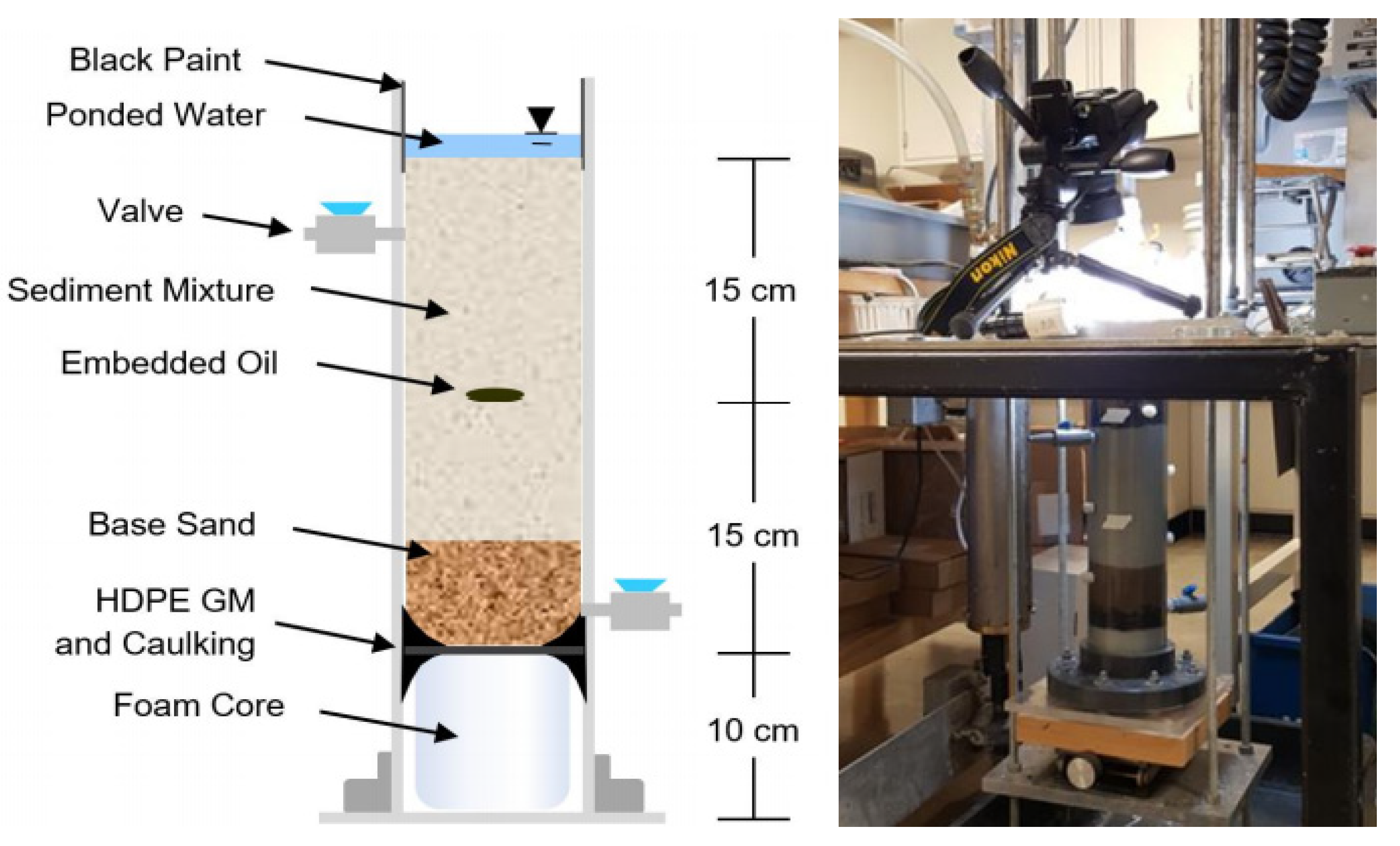
Sheen development videos were taken under anticipated field conditions (Figure 1). For the videos, oil was embedded 15 cm deep in a water-sediment column made up of a synthetic sediment mixture. A direct push probe with air or water injection was used to disturb the sediments and create a sheen from oil deposited into sediment in a 4-inch PVC tube. Three variations of the sediment mixture were considered, medium and fine sand mix, fine sand and fine (silt and clay) mix, and only fine (silt and clay) mix. Five crude oils of varying viscosities (2.21 cSt, 5.12 cSt, 66.3 cSt, 76.0 cSt, 469 cSt at 40 °C) were used to cover a range of oil types and ages expected in the field [22]. Different volumes of oil were placed in the sediments to produce sheens of higher or lower thickness as this impacts sheen color and form. The videos were taken using a digital single-lens reflex camera (Nikon DX D7200 with AF-S NKKOR 18–140 mm 1:3.5–5.6 G ED XR Lens) with a cool compact fluorescent lamp (CFL) lightbulb as the light source [22]. The average distance from the lens to the water surface is around 30 cm [22].
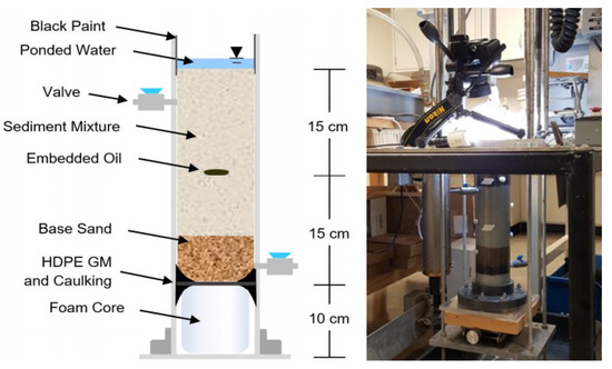
Figure 1.
Schematic of water-sediment column experimental design including the lighting and image collection in the laboratory OS-SS setup.
3.1.2. Image Dataset Preparation
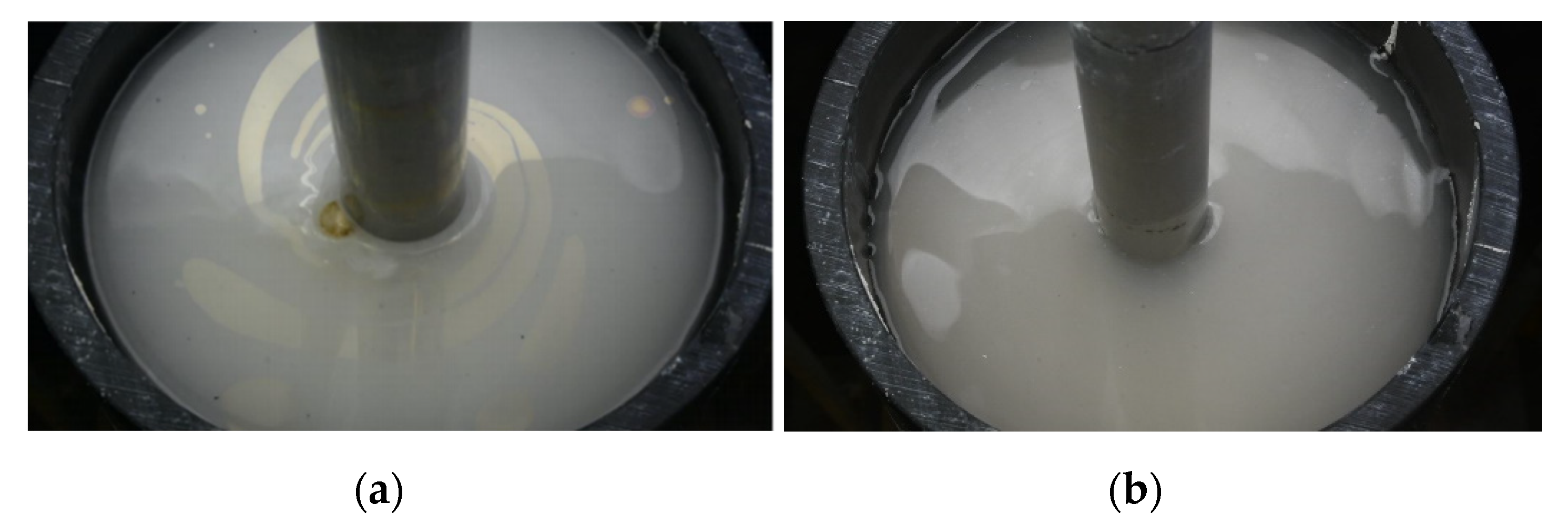
Based on the oil sheen videos, one frame of each second of the videos was scraped to create an efficient and nonredundant image dataset. In the data cleaning process, the blurry pictures and pictures where the water surface is obstructed, e.g., by experimenter’s hands, were deleted. The photos were labeled manually as “with Sheen” or “no Sheen”, based on expert opinion about the presence of the sheen (Figure 2). The total number of pictures extracted from the videos was 3398, which includes 1877 images labeled as “with Sheen” and 1521 images labeled as “no Sheen”. After randomizing, 90 percent of the data were used for training and 10 percent for testing. To obtain reliable performance of the method, training and testing datasets were independent.
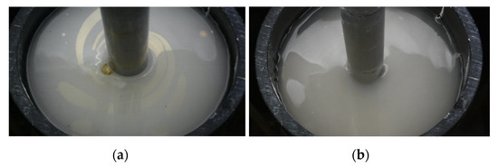
Figure 2.
Example of surface water in the OS-SS setup showing a (a) “with sheen” image and a (b) “no sheen” image used to create the surface sheen image library for the CNN model development.
3.1.3. Data Preprocessing
To develop a model with the best performance, the images were preprocessed before use in the model. The pre-processing methods included redefining the size of the images, data augmentation, normalization, and other operations. A CNN searches for thousands of patterns from the data and the patterns a model can find are related to the image size [39]. As our pre-trained model’s input image size is 224 × 224 × 3 (RGB image), the size of oil sheen images would be defined as 224 × 224 × 3 for training and testing to ensure the best transfer of the learned knowledge for our task. We normalized the tensor image using mean and standard deviation to obtain data within a range and reduce the skewness which helps the model to learn faster and more efficiently.
3.2. Oil Sheen Prediction Neural Network (OS-Net)
To build a deep neural network with better performance on oil sheen detection, we use residual block as basic element to overcome the vanishing gradient problem. To further improve the accuracy with limited oil sheen dataset, we use transfer learning strategies and explore the performance of different learning strategy on oil sheen detection.
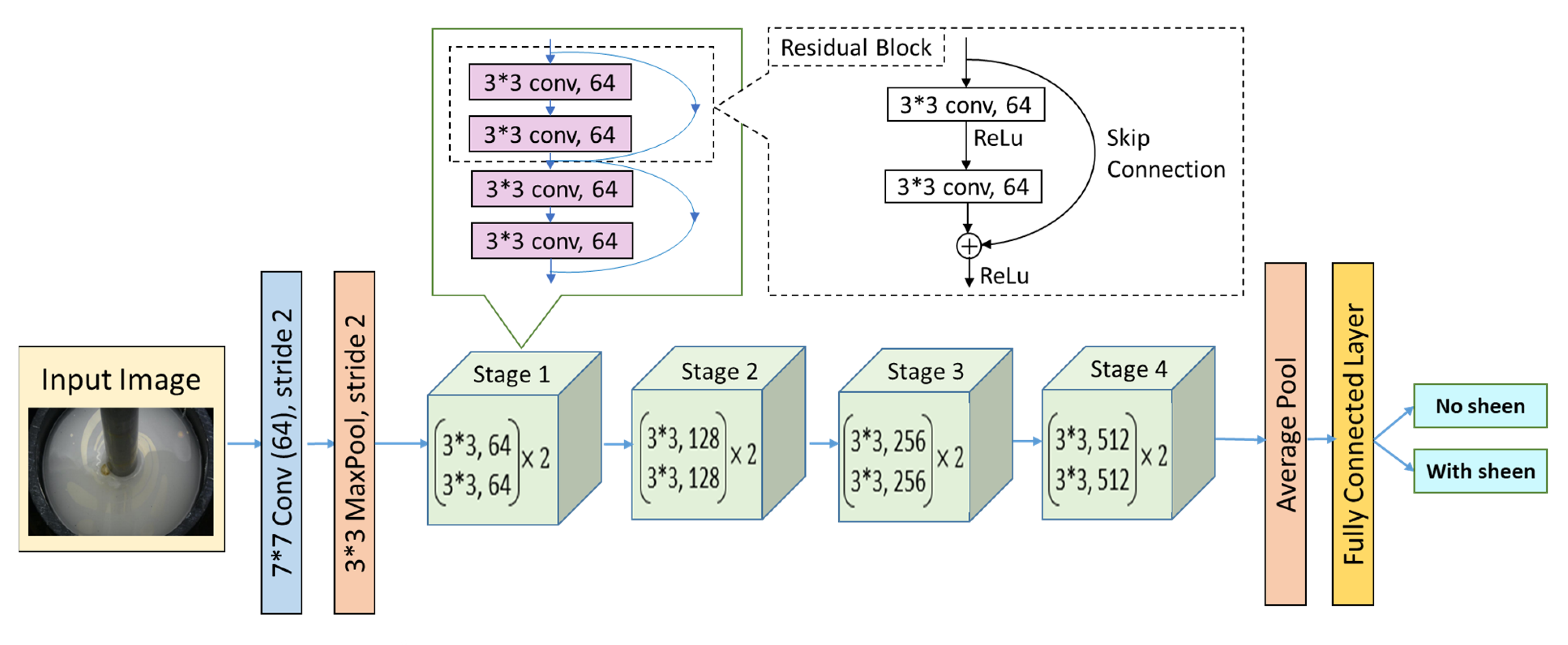
The OS-Net includes 18 convolutional layers with 8 residual blocks (Figure 3), which is a deep while easy-to-train neural network with a more powerful learning capacity.

Figure 3.
OS-Net architecture.
OS-Net has a traditional classification network architecture (see Figure 3). OS-Net has the first convolutional layer with 64 kernels (size = 7 × 7, stride = 2), followed by a maximum pooling layer (size = 3 × 3, stride = 2) to reduce the input oil sheen image size from 224 × 224 to a feature matrix of 56 × 56. The model backbone consists of 4 stages. Each stage consists of 2 residual blocks and each residual block has two 3 × 3 convolutional layers with skip connection. The penultimate layer is an average pooling layer to down sample the detection of features in feature maps. The last fully connected layer is also the output layer, which provides the classification prediction. We use Softmax to obtain the binary prediction result (‘No sheen’ or ‘With sheen’).
To accelerate the training and achieve higher accuracy, we use transfer learning strategy, which borrowed the learned general visual feature extraction knowledge from a larger dataset. The model starts with the pre-trained parameters using the ImageNet dataset and then adjusts these parameters to suit the oil sheen prediction task instead of starting the learning process from scratch with random parameter initialization. We explore the effectiveness of different strategies of transfer learning to gain the best OS-Net. These three strategies all used the same initial OS-Net architecture (Figure 3), but each model was trained differently and compared to the case without transfer learning. (Case A) OS-Net Without Transfer Learning. The model was trained from scratch on close-proximity oil sheen image dataset with random initialized parameters. (Case B) OS-Net With Transfer Learning Feature Extraction Strategy. We used the pre-trained model as a feature extractor to transfer the similar feature extraction ability learned from ImageNet to our model. Specifically, we pre-trained our OS-Net on ImageNet, modified the fully connected layers as shown in Figure 3, froze all the networks except the final layer, and then trained the model on our dataset. (Case C) OS-Net With Transfer Learning Fine-tuning Strategy. We used the pre-trained model as the starting point of training, then fine tuned all parameters for the target task. Specifically, we pre-trained our OS-Net on ImageNet, modified the fully connected layers, unfroze all layers, then trained the model on our oil sheen dataset.
In the training process, cross entropy was used as a loss function to update model weights w. The cross-entropy function is given in Equation (1) [40],
where M represents the number of classes, true probability p is the true label (no oil or with oil), and q is the predicted value of the current model.
The model was trained using the stochastic gradient descent (SGD) optimization algorithm [40,41]. The SGD updates the network parameters (weights and biases) to minimize the loss function. This algorithm is defined as:
where w donates any trainable variable (W or B), t is the current time step (algorithm iteration), and α is the learning rate.
3.3. OS-Net Performance Evaluation
Four performance evaluation metrics were employed to assess the OS-Net performance, including accuracy (Equation (3)), precision (Equation (4)), recall (Equation (5)), and F1 score (Equation (6)). Accuracy is the ratio of correctly predicted observations to the total observations. Precision is the ratio of correctly predicted positive observations to the total predicted positive observations. Recall is the ratio of correctly predicted positive observations to all observations in actual class. F1 Score is the weighted average of precision and recall [42] and is a reliable and robust indicator for accurate model measurements. The range of the F-1 score is from 0 to 1, with 0 being the worst possible and 1 being the best.
where TP refers to true positives, TN refers to true negatives, FP refers to positives, and FN refers to false negatives.
3.4. Real-Time Video Oil Sheen Prediction (VOS-Net)
Based on the OS-Net, we developed a real-time video-based oil sheen prediction system (VOS-Net). The input of the VOS-Net is sheen formation video and the output is the real-time prediction result. Given a video input, the VOS-Net classifies the images every few frames based on image extraction frequency parameter.
The latency of the VOS-Net may delay the prediction results if the model predicts frame by frame. To achieve real-time prediction, an appropriate image extraction frequency will have to be set to offset the delay. When the interval between image extractions is greater than the model inference time, predictions would not be delayed.
While recall is 100% and false negatives are not likely, the precision is not 100% so some false-positive results could occur and a method was developed to address this potential.
We combined oil sheen domain knowledge with our machine learning algorithm to improve the prediction accuracy. When oil leaks from the sediment in OS-SS, the oil will spread out rapidly on the water surface to form sheen. The appearance of oil sheen can sometimes be fleeting, disappearing after a few seconds, or it can persist for a longer period [22]. Thus, if the sheen only appears for one frame (the video includes 60 frames per second), the prediction may be a false positive. We set a filter with kernel size k, where k represents the threshold of positive prediction. We suppressed the positive prediction until k successive positive predictions occurred. The kernel size k can be adjusted to control the sensitivity of VOS-Net to avoid false positives and increase predictive accuracy.
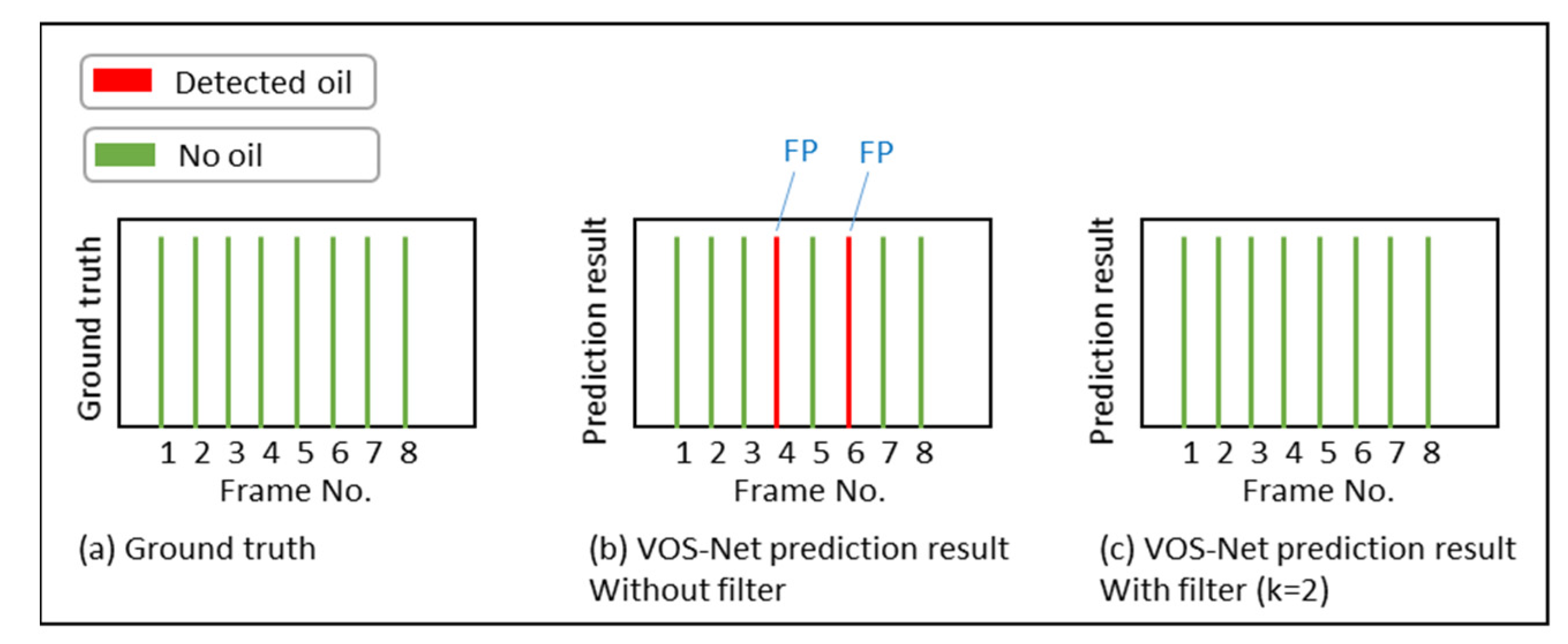
Figure 4 shows how the VOS-Net filter works. The VOS-Net predicts the oil sheen every 60 frames (~1 s) and records the result. Figure 4a shows the ground truth (b) and (c) show the VOS-Net prediction result with the different filters applied. The red line represents the model’s prediction of “with sheen”, while the green line depicts a model result of “no sheen”. The ground truth is when no oil appears in the following frames. Without applying a filter, (b), VOS-Net could have a false positive (red lines). After applying a filter, (c), the VOS-Net can reduce the false-positive incidence and achieve higher accuracy.
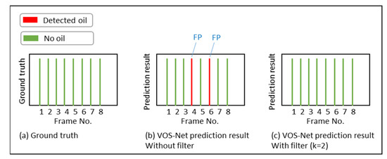
Figure 4.
VOS-Net filter performance demonstration. Screening out single false-positive events improves the model accuracy to 99%.
4. Results
4.1. OS-Net Performance
Table 1 shows the accuracy, precision, recall, and F-1 score for three models: (A) OS-Net Without Transfer Learning; (B) OS-Net With Transfer Learning Feature Extraction Strategy; (C) OS-Net With Transfer Learning Fine-tuning Strategy. In model development, we use grid search for hyperparameter tuning for each of the three models mentioned above. Then, we obtain the best hyperparameter settings and the corresponding best model performance (Table 1) for each of the models. The best initial learning rate of the best OS-Net without transfer learning is 0.002, which is larger than the best initial learning rate of the OS-Net with ImageNet pretrained model (0.001). We also use a learning rate schedule to adjust the learning rate during training. The learning rate will decrease rapidly in the first few epochs, then gradually reduce as the iteration continues to make the model more stable. The settings of grid search values for hyperparameters tuning in each model are listed in Table S3. The best hyperparameters for our best OS-Net model are listed here: the momentum factor is 0.9, the initial learning rate is 0.001, epochs are 30, and the batch size is 16.

Table 1.
Model evaluation result.
From the results presented in Table 1, the OS-Net With Transfer Learning and the Fine-tuning Strategy approach performed best. Therefore, we selected OS-Net With Transfer Learning and the Fine-tuning Strategy as our final OS-Net.
The OS-Net is robust for the oil sheen classification task in our laboratory-generated dataset, accurately predicting the oil sheen appearance on the water surface in our OS-SS prototype. The accuracy and F-1 score of the OS-Net are up to 99%. The model can efficiently extract the low-level features and high-level features from images. The recall rate is up to 100%, which means that there are no false negatives.
The reason why OS-Net Without Transfer Learning has relatively low accuracy, compared to the final OS-Net, may be a result of the relatively small size of our oil sheen image dataset. When we trained the model from scratch on our oil sheen image dataset, the knowledge that the model can learn is limited, leading to overfitting and a lack of generalizability. The model can only fit well with similar data but not data the model has never seen before. Here, we also tried a “warm-up” training approach to reduce variance in the early stage of training and achieve better performance for the OS-Net without transfer learning model, but the final accuracy was not improved. This result indicates the role of transfer learning is more than just “warming up” the weights better. In contrast, the OS-Net With Transfer Learning and the Fine-tuning Strategy is pre-trained on the ImageNet dataset, which has millions of images, providing the model with a better generalization ability. The model was then fine tuned on the specific oil sheen dataset to adjust its parameters to improve the specific oil sheen prediction task. This suggests that transfer learning is helpful to transfer the extracted basic features from ImageNet to our new task. Even though the high-level features have large visual differences between the two tasks (ImageNet has no oil sheen images), the basic feature (low-level patterns, e.g., edges, color patterns, elementary shapes) extraction ability is shared across tasks.
It is worth noting that the performance of the OS-Net With Transfer Learning Feature Extraction Strategy did not improve significantly compared to the OS-Net Without Transfer Learning. This may be due to the large gap between the target (close-proximity oil sheen) images and the pre-trained model’s ImageNet dataset. The types of advanced features (middle or high level) that need to be extracted from the two datasets are not the same, so using the pre-trained model as the feature extractor may not be ideal.
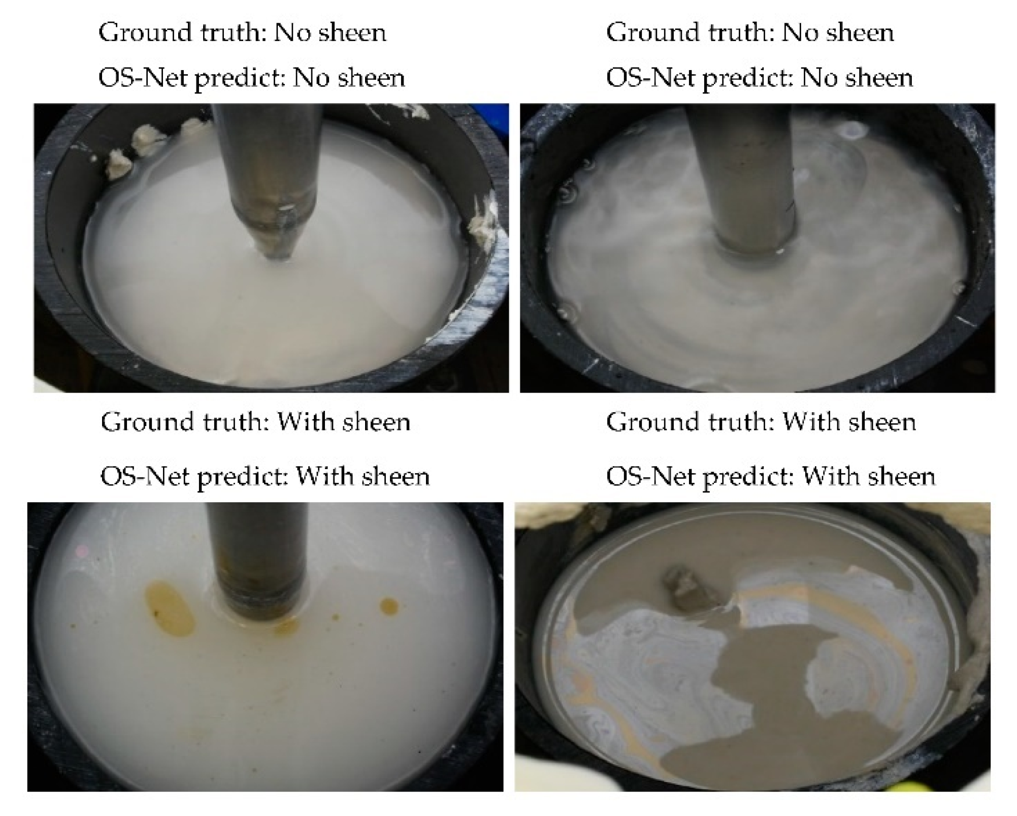
Figure 5 shows sample images with the ground truth label and the OS-Net prediction results. Images with oil sheen or without oil sheen can be correctly classified by the OS-Net. Since the water surface is moving during the video recording and the shape and color of the sheen will be constantly changing during the video, the variance increases. Our OS-Net performs well under these conditions, indicating the robustness and generalizability of our method.
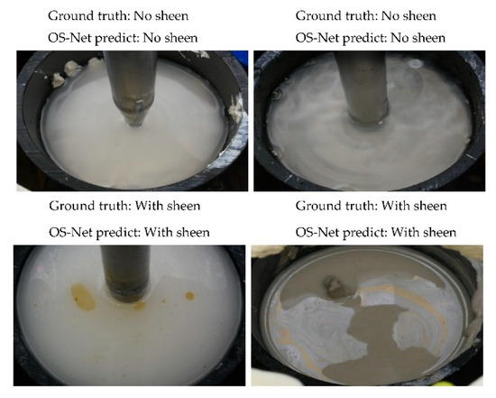
Figure 5.
Example oil sheen image ground truth and OS-Net prediction results.
4.2. VOS-Net
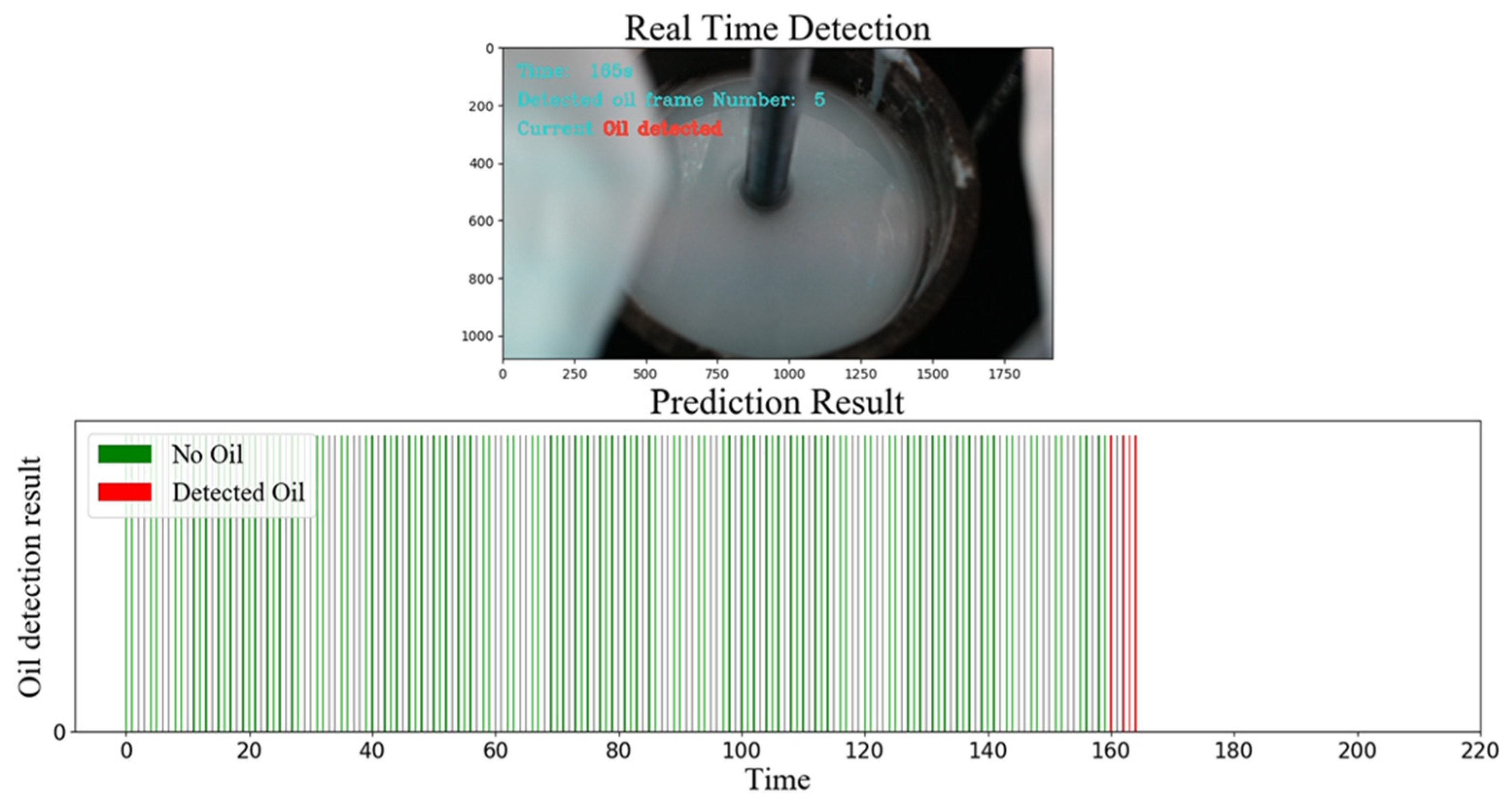
Finally, a video-based real-time oil sheen detection algorithm (VOS-Net) was developed, providing users with a visual image with oil sheen detection result. Figure 6 demonstrates the VOS-Net functions. Given a video input, the VOS-Net will show the image extracted on the top window with time, detected frame number, and prediction result of the current frame. Above the video image, a record of the prediction result is shown.
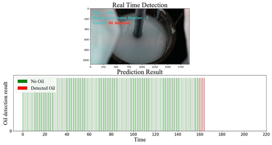
Figure 6.
VOS-Net prediction window and result; a demo of VOS-Net result is available at https://youtu.be/kCZnMAYBByk (accessed on 15 July 2022).
The image extraction frequency can be adjusted manually, based on the performance of the users’ computer, to offset the latency effect of the VOS-Net. In the test, the model inference time to predict one image is 0.03–0.04 s (2.4 frames on average). The shortest time that oil sheen appears on the water surface in OS-SS is 3 s, based on our lab experiment. In this case, setting the image extraction frequency anywhere from 3 frames to 180 frames, the VOS-Net can achieve real-time prediction on each image. To achieve higher accuracy and avoid response latency, we suggest selecting the image extraction frequency parameter in a range from 30 to 60 (0.5 s to 1 s).
When we applied a filter (k) larger than two, the filter could efficiently suppress false-positive predictions to increase the accuracy of VOS-Net.
5. Discussion and Conclusions
This paper introduces the concept of a subaquatic sediment oil sheen screening system (OS-SS) and develops a novel oil sheen detection system to autonomously monitor the sediment’s sheening potential after disturbance with compressed air or water. The OS-SS also provides reliable real-time oil sheen video. Based on the videos from OS-SS, we successfully created a new close-proximity oil sheen image dataset, which includes thousands of oil sheen images (five types of oil sheen formation details under different environmental conditions in the lab). This dataset can become a resource for a broad range of oil-sheen-modeling-related research.
We developed an Oil Sheen Prediction Neural Network (OS-Net), a Convolutional Neural Network (CNN), combined with transfer learning, to achieve real-time image-based oil sheen prediction from video and applied the model in a simulation of the OS-SS. The accuracy of OS-Net was up to 99%. To mitigate false positives from the video stream, we employed a sensitivity filter in the VOS-Net. Thus, our VOS-Net can output accurate feedback to monitor the formation of an oil sheen present given a video stream, even if that formation is short lived in the order of a few seconds to a few tens of seconds. The kernel size, a hyperparameter-insensitive filter, can be adjusted to control the sensitivity of VOS-Net to avoid false positives. Moreover, we determined the image extraction frequency parameters in VOS-Net needed to avoid model prediction latency and provide real-time feedback. To further reduce the model reference time and extend the range of image extraction frequency, we tried to use depth-wise convolution to replace the regular convolution in the OS-Net to reduce the number of parameters and computations. As a result, compared to the original OS-Net, the accuracy of the OS-Net model with depth-wise convolution was reduced by 1.66% and the average latency was reduced by 2.65%. The result suggests that depth-wise convolution can reduce the inference time. How to use depth-wise convolution to reduce model latency while also ensuring accuracy will be a good question to explore in the future. Model quantization, mapping values from a larger set to a smaller one to reduce the floating point, is another approach worth trying to reduce the memory and complexity of computations in the future.
The OS-SS with VOS-Net could be easily applied in the field, potentially being deployed on an autonomous watercraft to map the spatial distribution of sediment sheening potential in rivers, creeks, fords, and shallow waters [43]. The VOS-Net can automatically show the real-time result and record the detection result along with the GPS location to determine the precise location of the sediments with high sheening potential. The OS-SS with VOS-Net could be an efficient tool for mapping problematic regions of subaquatic sediments for further evaluation or remediation. The autonomous nature of the approach also makes it ideal for deployment in difficult-to-reach terrains. Moreover, as our OS-Net is based on visible light images, the requirements and costs for image collection equipment are low. The algorithms could be further explored to be used with a cellphone camera to detect the oil sheen on the water or in other similar scenarios, such as oil drilling or storm runoff in the future.
Furthermore, our results indicated that combining residual blocks with transfer learning helped our OS-Net to overcome the challenge of limited datasets to obtain a deeper and more robust neural network and achieve high accuracy. The appropriate transfer learning strategy was related to the pre-training and task datasets. When there is a significant gap between the two datasets, a fine-tuning transfer learning strategy improved the accuracy of the model. The improved performance of OS-Net is a good example. Data augmentation can also potentially enhance the training dataset for the small dataset. In our case, using random horizontal flip alone improved the model’s accuracy by 0.65% (SI Table S2).
Although the model has high accuracy, there are still some limitations. The data distribution likely does not represent the full range of actual data distribution that may be encountered when probing different natural subaquatic environments because of the range of environmental parameters that may be encountered (e.g., different types of oil, different degrees of weathering, different natural organic matter content, and natural biofilm formation). Thus, the domain gap between the lab data during training and the video from actual field samples may influence the accuracy. Future work can overcome these challenges by enlarging the oil sheen dataset collected with different natural conditions, including a range of videos and images taken for field sheen events using the OS-SS.
Supplementary Materials
The following supporting information can be downloaded at: https://www.mdpi.com/article/10.3390/app12178865/s1, Table S1: Input data summary table. Table S2: OS-Net performance under different data augmentation methods. Table S3: OS-Net hyperparameters tuning grid search values. Figure S1: VOS-Net prediction results. The X axis shows the prediction index with time (1 prediction/s) and the Y axis shows the VOS-Net prediction result. The black line represents the region where there was oil sheen present. Ground truth labels are shown at the top of each region.
Author Contributions
J.D., P.B., N.S. and T.P.H.; Data curation, K.S.; Formal analysis, J.D., J.S. and Y.G.; Funding acquisition, P.B., N.S., T.P.H. and G.V.L.; Investigation, K.S. and G.V.L.; Methodology, J.D., K.S. and G.V.L.; Supervision, J.S.; Validation, J.D. and Y.G.; Writing—review & editing, K.S., J.S., Y.G., P.B., N.S., T.P.H. and G.V.L. All authors have read and agreed to the published version of the manuscript.
Funding
This research was funded by Chevron.
Data Availability Statement
The data presented in this study are available on request from the corresponding author. The data are not publicly available due to agreements in place with the study sponsor.
Conflicts of Interest
The authors declare no conflict of interest.
References
- Neff, J.M. Composition and fate of petroleum and spill-treating agents in the marine environment. In Synthesis of Effects of Oil on Marine Mammals; Battelle Memorial Institute: Ventura, CA, USA, 1988; pp. 1–33. [Google Scholar] [CrossRef]
- Romero, I.C.; Schwing, P.T.; Brooks, G.R.; Larson, R.A.; Hastings, D.W.; Ellis, G.; Goddard, E.A.; Hollander, D.J. Hydrocarbons in deep-sea sediments following the 2010 deepwater horizon blowout in the Northeast Gulf of Mexico. PLoS ONE 2015, 10, e0128371. [Google Scholar] [CrossRef] [PubMed]
- National Research Council. Oil in the Sea III: Inputs, Fates, and Effects; National Academies Press: Washington, CA, USA, 2003. [Google Scholar] [CrossRef]
- Picou, J.S.; Gill, D.A.; Dyer, C.L.; Curry, E.W. Disruption and stress in an alaskan fishing community: Initial and continuing impacts of the exxon valdez oil spill. Ind. Crisis Q. 2016, 6, 235–257. [Google Scholar] [CrossRef]
- Adams, A. PAGe 2. Summary of Information Concerning the Ecological and Economic Impacts of the BP Deepwater Horizon Oil Spill Disaster New England Coral Canyons and Seamounts Area. NRDC Issue Paper. 19 June 2015. Available online: https://www.nrdc.org/resources/summary-information-concerning-ecological-and-economic-impacts-bp-deepwater-horizon-oil (accessed on 30 July 2021).
- Effects of Oil Spills: What Impact Does it Have on Wildlife and Humans? Available online: https://www.offshore-technology.com/features/effects-oil-spills/ (accessed on 30 July 2021).
- Nance, E.; King, D.; Wright, B.; Bullard, R.D. Ambient air concentrations exceeded health-based standards for fine particulate matter and benzene during the deepwater horizon oil spill. J. Air Waste Manag. Assoc. 2016, 66, 224–236. [Google Scholar] [CrossRef] [PubMed]
- Al-Shammari, A.; Levin, E.; Shults, R. Oil spills detection by means of uas and low-cost airborne thermal sensors. ISPRS Ann. Photogramm. Remote Sens. Spat. Inf. Sci. 2018, 4, 293–301. [Google Scholar] [CrossRef]
- Del Frate, F.; Petrocchi, A.; Lichtenegger, J.; Calabresi, G. Neural networks for oil spill detection using ERS-SAR data. IEEE Trans. Geosci. Remote Sens. 2000, 38, 2282–2287. [Google Scholar] [CrossRef]
- Zeng, K.; Wang, Y. A Deep convolutional neural network for oil spill detection from spaceborne SAR images. Remote Sens. 2020, 12, 1015. [Google Scholar] [CrossRef]
- Fiscella, B.; Giancaspro, A.; Nirchio, F.; Pavese, P.; Trivero, P. Oil spill detection using marine SAR images. Int. J. Remote Sens. 2010, 21, 3561–3566. [Google Scholar] [CrossRef]
- Vespe, M.; Greidanus, H. SAR image quality assessment and indicators for vessel and oil spill detection. IEEE Trans. Geosci. Remote Sens. 2012, 50 Pt 2, 4726–4734. [Google Scholar] [CrossRef]
- Topouzelis, K.N. Oil spill detection by SAR images: Dark formation detection, feature extraction and classification algorithms. Sensors 2008, 8, 6642–6659. [Google Scholar] [CrossRef]
- Kubat, M.; Holte, R.C.; Matwin, S. Machine learning for the detection of oil spills in satellite radar images. Mach. Learn. 1998, 30, 195–215. [Google Scholar] [CrossRef]
- Singha, S.; Bellerby, T.J.; Trieschmann, O. Satellite oil spill detection using artificial neural networks. IEEE J. Sel. Top. Appl. Earth Obs. Remote Sens. 2013, 6, 2355–2363. [Google Scholar] [CrossRef]
- De Kerf, T.; Gladines, J.; Sels, S.; Vanlanduit, S. Oil spill detection using machine learning and infrared images. Remote Sens. 2020, 12, 4090. [Google Scholar] [CrossRef]
- Al-Ruzouq, R.; Gibril, M.B.A.; Shanableh, A.; Kais, A.; Hamed, O.; Al-Mansoori, S.; Khalil, M.A. Sensors, features, and machine learning for oil spill detection and monitoring: A review. Remote Sens. 2020, 12, 3338. [Google Scholar] [CrossRef]
- Bukin, O.; Proschenko, D.; Korovetskiy, D.; Chekhlenok, A.; Yurchik, V.; Bukin, I. Development of the artificial intelligence and optical sensing methods for oil pollution monitoring of the sea by drones. Appl. Sci. 2021, 11, 3642. [Google Scholar] [CrossRef]
- Jiao, Z.; Jia, G.; Cai, Y. A new approach to oil spill detection that combines deep learning with unmanned aerial vehicles. Comput. Ind. Eng. 2019, 135, 1300–1311. [Google Scholar] [CrossRef]
- Alharam, A.; Almansoori, E.; Elmadeny, W.; Alnoiami, H. Real time AI-based pipeline inspection using drone for oil and gas industries in Bahrain. In Proceedings of the 2020 International Conference on Innovation and Intelligence for Informatics, Computing and Technologies (3ICT), Sakheer, Bahrain, 20–21 December 2020. [Google Scholar] [CrossRef]
- Sale, T.; Hopkins, H.; Andrew, K. Managing Risk at LNAPL Sites. Am. Pet. Inst. Soil Groundw. Res. Bull. 2018, 18, 51–53. [Google Scholar]
- Sitler, K.; Scalia, J.; Sale, T. Identification and Validation of Screening Methods for Assessment of the Sheening Potential of Embedded Oil in Sediments; Colorado State University: Fort Collins, CO, USA, 2020. [Google Scholar]
- He, K.; Zhang, X.; Ren, S.; Sun, J. Deep residual learning for image recognition. In Proceedings of the IEEE Conference on Computer Vision and Pattern Recognition (CVPR), Las Vegas, NV, USA, 27–30 June 2016; 2016; pp. 770–778. [Google Scholar]
- Alzubaidi, L.; Zhang, J.; Humaidi, A.J.; Al-Dujaili, A.; Duan, Y.; Al-Shamma, O.; Santamaría, J.; Fadhel, M.A.; Al-Amidie, M.; Farhan, L. Review of deep learning: Concepts, CNN architectures, challenges, applications, future directions. J. Big Data 2021, 8, 1–74. [Google Scholar] [CrossRef]
- Gu, J.; Wang, Z.; Kuen, J.; Ma, L.; Shahroudy, A.; Shuai, B.; Liu, T.; Wang, X.; Wang, L.; Wang, G.; et al. Recent Advances in Convolutional Neural Networks. Pattern Recognit. 2018, 77, 354–377. [Google Scholar] [CrossRef] [Green Version]
- Zhiqiang, W.; Jun, L. A review of object detection based on convolutional neural network. In Proceedings of the 2017 36th Chinese Control Conference (CCC), Dalian, China, 26–28 July 2017; pp. 11104–11109. [Google Scholar] [CrossRef]
- Rehman, S.; Ajmal, H.; Farooq, U.; Ain, Q.U.; Riaz, F.; Hassan, A. Convolutional neural network based image segmentation: A review. Pattern Recognit. Track. XXIX 2018, 10649, 191–203. [Google Scholar] [CrossRef]
- Gao, Y.; Mosalam, K.M. Deep transfer learning for image-based structural damage recognition. Comput. Civ. Infrastruct. Eng. 2018, 33, 748–768. [Google Scholar] [CrossRef]
- Hussain, M.; Bird, J.J.; Faria, D.R. A Study on CNN transfer learning for image classification. Adv. Intell. Syst. Comput. 2018, 840, 191–202. [Google Scholar] [CrossRef]
- Zheng, J.; Yang, G.; Huang, Y.; Liu, L.; Hong, G.; Qiu, Z.; Liu, S. Research of water body turbidity classification model for aquiculture based on transfer learning. J. Phys. Conf. Ser. 2021, 1757, 012004. [Google Scholar] [CrossRef]
- Deng, J.; Dong, W.; Socher, R.; Li, L.-J.; Kai, L.; Li, F.-F. ImageNet: A large-scale hierarchical image database. IEEE Comput. Soc. 2010, 2009, 248–255. [Google Scholar] [CrossRef]
- Simonyan, K.; Zisserman, A. Very deep convolutional networks for large-scale image recognition. arXiv 2014, arXiv:1409.1556. [Google Scholar]
- Krizhevsky, A.; Sutskever, I.; Hinton, G.E. ImageNet Classification with Deep Convolutional Neural Networks. Commun. ACM 2017, 60, 84–90. [Google Scholar] [CrossRef]
- Szegedy, C.; Liu, W.; Jia, Y.; Sermanet, P.; Reed, S.; Anguelov, D.; Erhan, D.; Vanhoucke, V.; Rabinovich, A. Going deeper with convolutions. In Proceedings of the IEEE Conference on Computer Vision and Pattern Recognition (CVPR), Boston, MA, USA, 7–12 June 2015; pp. 1–9. [Google Scholar] [CrossRef]
- Zhuang, F.; Qi, Z.; Duan, K.; Xi, D.; Zhu, Y.; Zhu, H.; Xiong, H.; He, Q. A comprehensive survey on transfer learning. Proc. IEEE 2019, 109, 43–76. [Google Scholar] [CrossRef]
- Yosinski, J.; Clune, J.; Bengio, Y.; Lipson, H. How transferable are features in deep neural networks? Adv. Neural Inf. Process. Syst. 2014, 4, 3320–3328. [Google Scholar]
- Best, N.; Ott, J.; Linstead, E.J. Exploring the efficacy of transfer learning in mining image-based software artifacts. J. Big Data 2020, 7, 1–10. [Google Scholar] [CrossRef]
- Gong, Z.; Zhong, P.; Hu, W. Diversity in machine learning. IEEE Access 2019, 7, 64323–64350. [Google Scholar] [CrossRef]
- Li, H.; Ellis, J.G.; Zhang, L.; Chang, S.-F. PatternNet: Visual pattern mining with deep neural network. In Proceedings of the 2018 ACM on International Conference on Multimedia Retrieval, Yokohama, Japan, 11–14 June 2018. [Google Scholar] [CrossRef]
- Rojas, R. The backpropagation algorithm. Neural Netw. 1996, 40, 149–182. [Google Scholar] [CrossRef]
- Cui, X.; Zhang, W.; Tüske, Z.; Picheny, M. Evolutionary stochastic gradient descent for optimization of deep neural networks. Adv. Neural Inf. Process. Syst. 2018, 2018, 6048–6058. [Google Scholar]
- Yacouby, R.; Axman, D. Probabilistic extension of precision, recall, and F1 score for more thorough evaluation of classification models. In Proceedings of the First Workshop on Evaluation and Comparison of NLP Systems, Punta Cana, Dominican Republic, 20 November 2020; pp. 79–91. [Google Scholar] [CrossRef]
- Valada, A.; Velagapudi, P.; Kannan, B.; Tomaszewski, C.; Kantor, G.; Scerri, P. Development of a low cost multi-robot autonomous marine surface platform. Springer Tracts Adv. Robot. 2014, 92, 643–658. [Google Scholar] [CrossRef] [Green Version]
Publisher’s Note: MDPI stays neutral with regard to jurisdictional claims in published maps and institutional affiliations. |
© 2022 by the authors. Licensee MDPI, Basel, Switzerland. This article is an open access article distributed under the terms and conditions of the Creative Commons Attribution (CC BY) license (https://creativecommons.org/licenses/by/4.0/).

