
A Novel Constant Power Factor Loop for Stable V/f Control of PMSM in Comparison against Sensorless FOC with Luenberger-Type Back-EMF Observer Verified by Experiments

Abstract
:1. Introduction
2. Mathematical Model of PMSM
3. Sensorless FOC with Luenberger-Type Back-EMF Observer
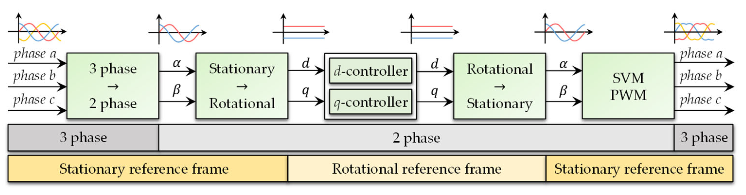
3.1. Sensorless FOC
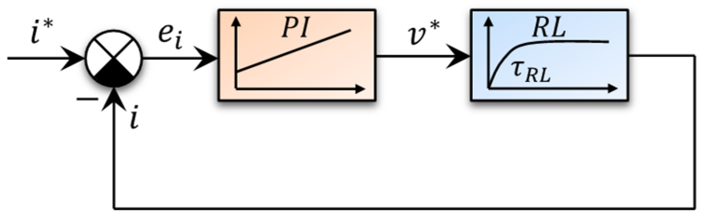
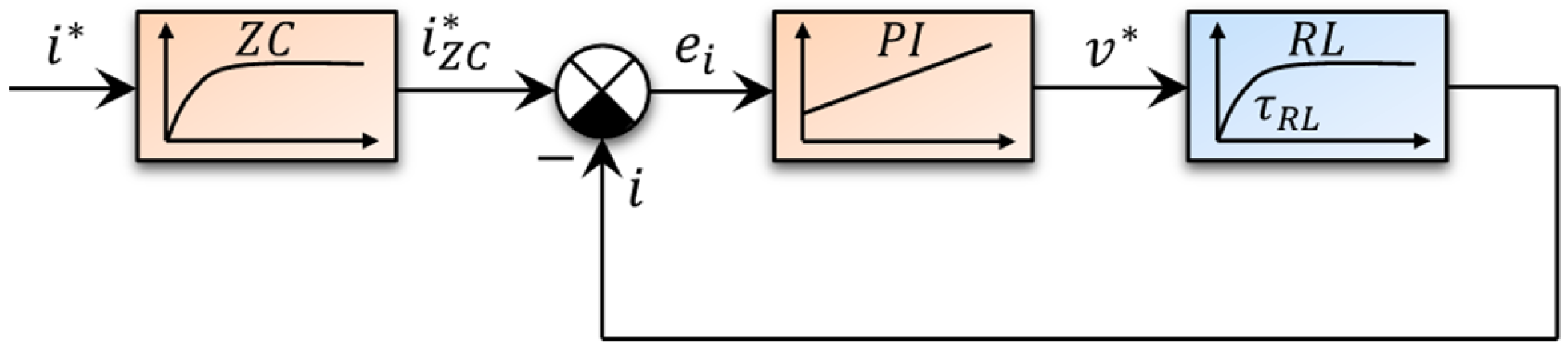
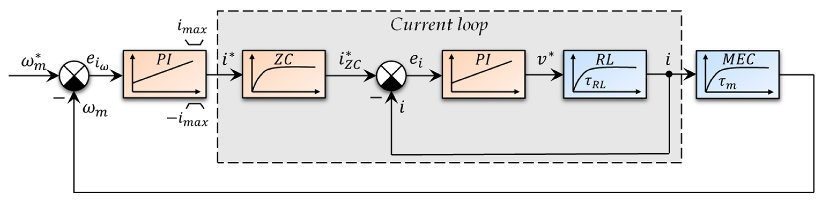
3.1.1. Current Loop
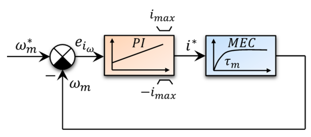
3.1.2. Speed Loop
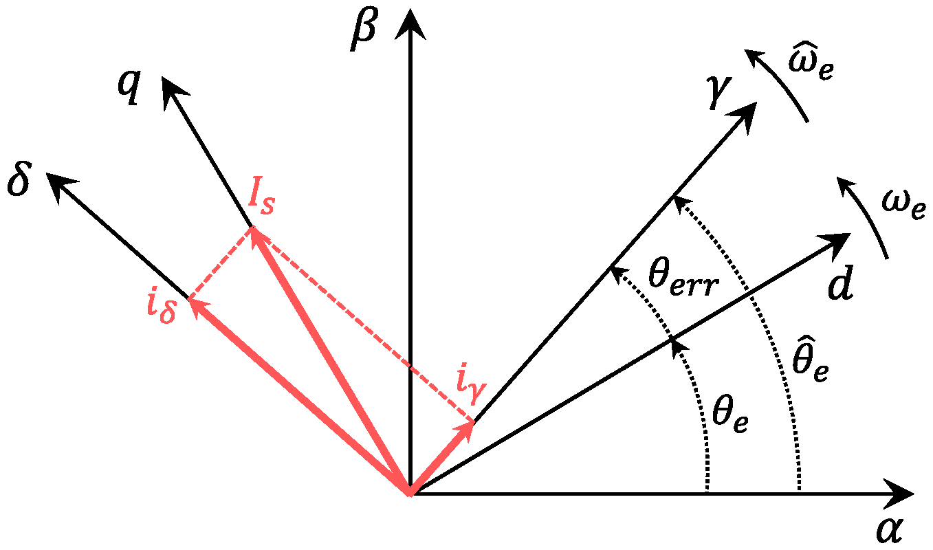
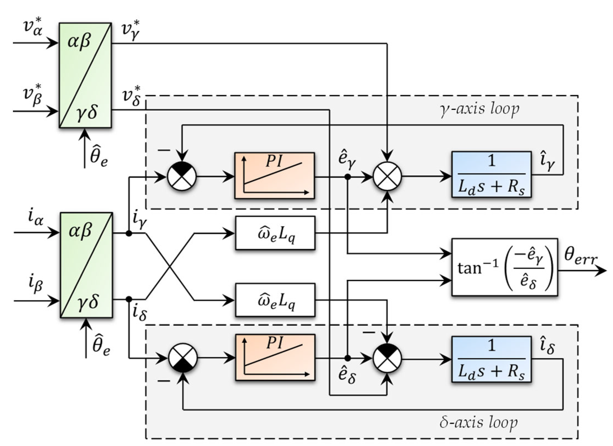
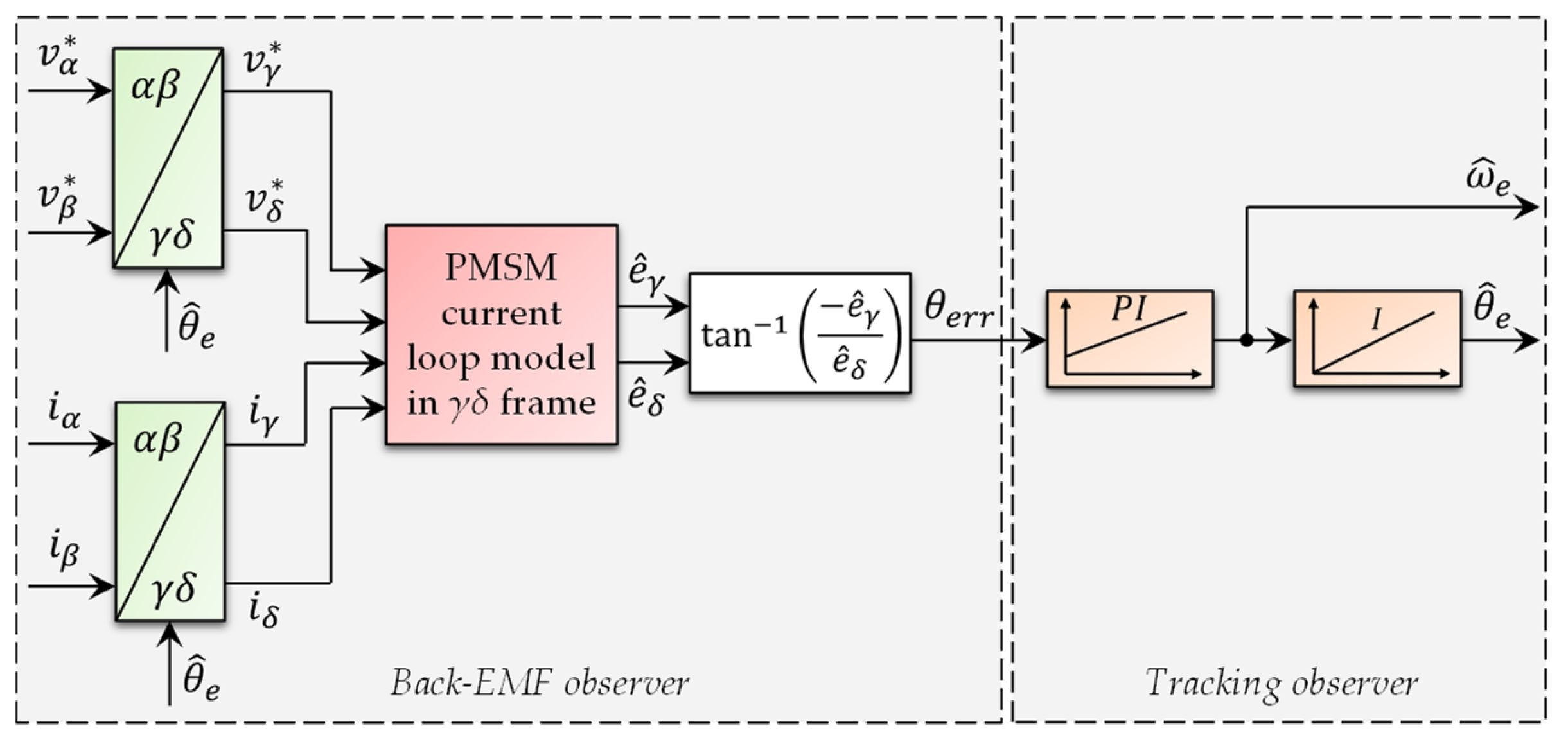
3.2. Luenberger-Type Back-EMF Observer
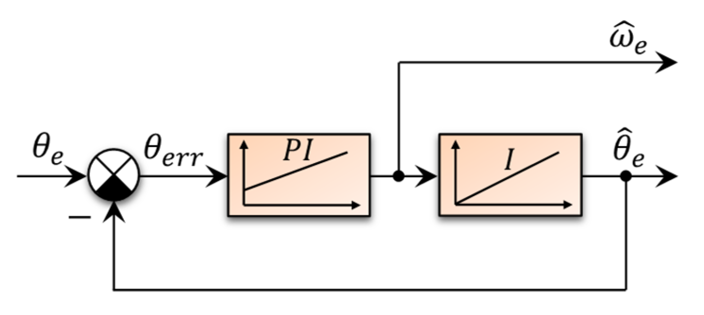
3.3. Tracking Observer
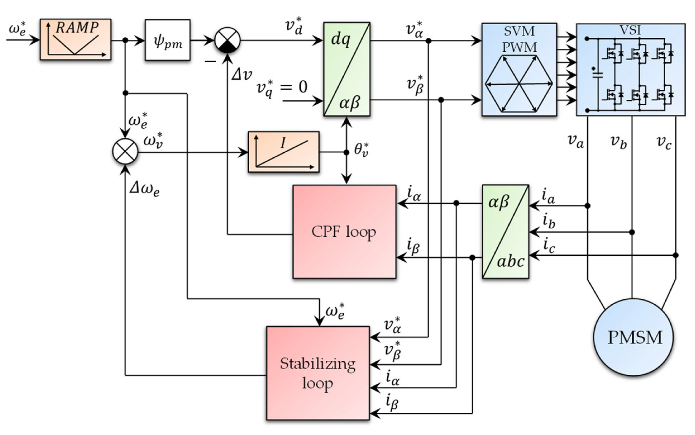
4. Stable V/f Control with Constant Power Factor Loop
- Instability of the system after exceeding a specific applied frequency;
- Low dynamic performance;
- Poor fault protection against stall detection and overcurrent.

| Control Structure | PI | I | Park | Clarke | Atan | Filters |
|---|---|---|---|---|---|---|
| Stable V/f control with constant power factor loop | 1 | 1 | 2 | 1 | 0 | 1 |
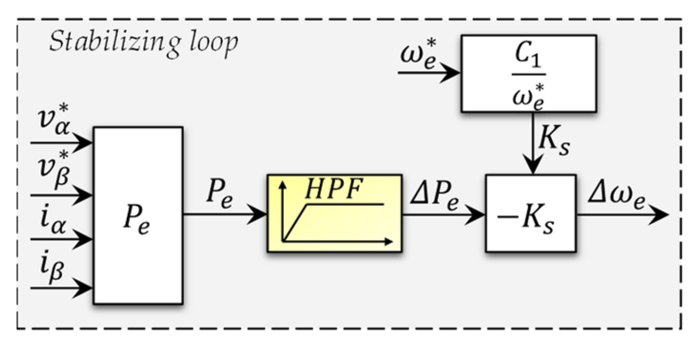
4.1. Stabilizing Loop
- DC link current;
- Actual rotor speed;
- Input active power.
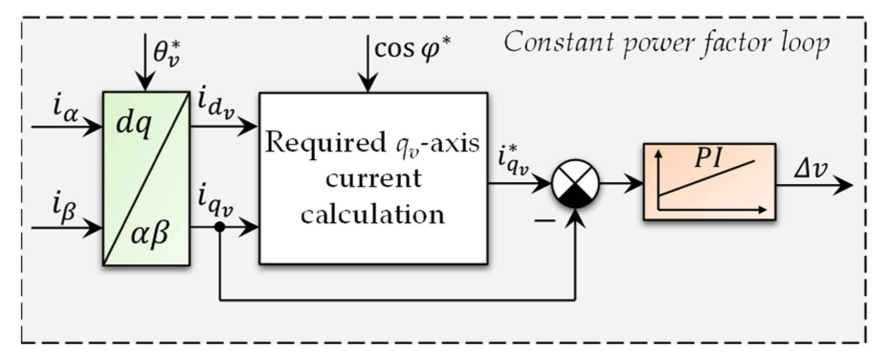
4.2. Constant Power Factor Control Loop
5. Experimental Results
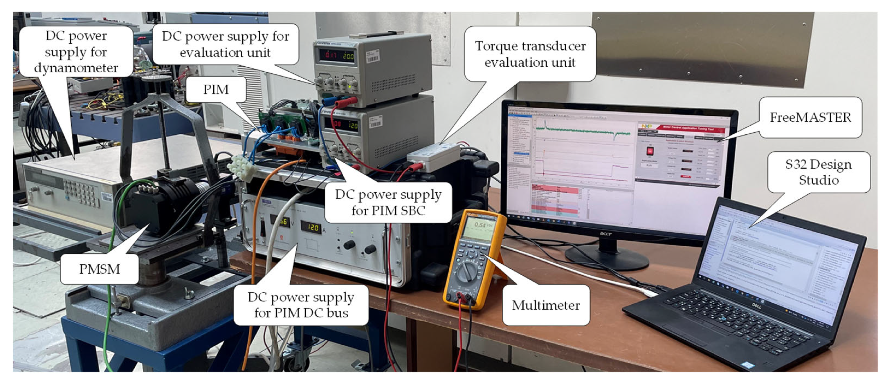
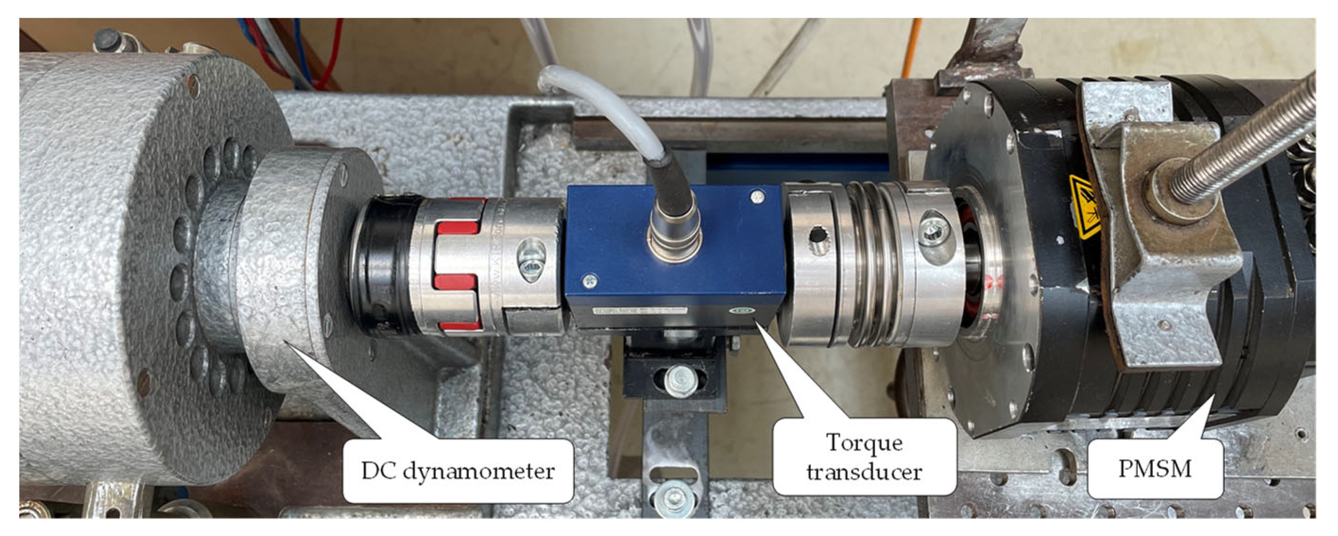
5.1. Experimental Setup
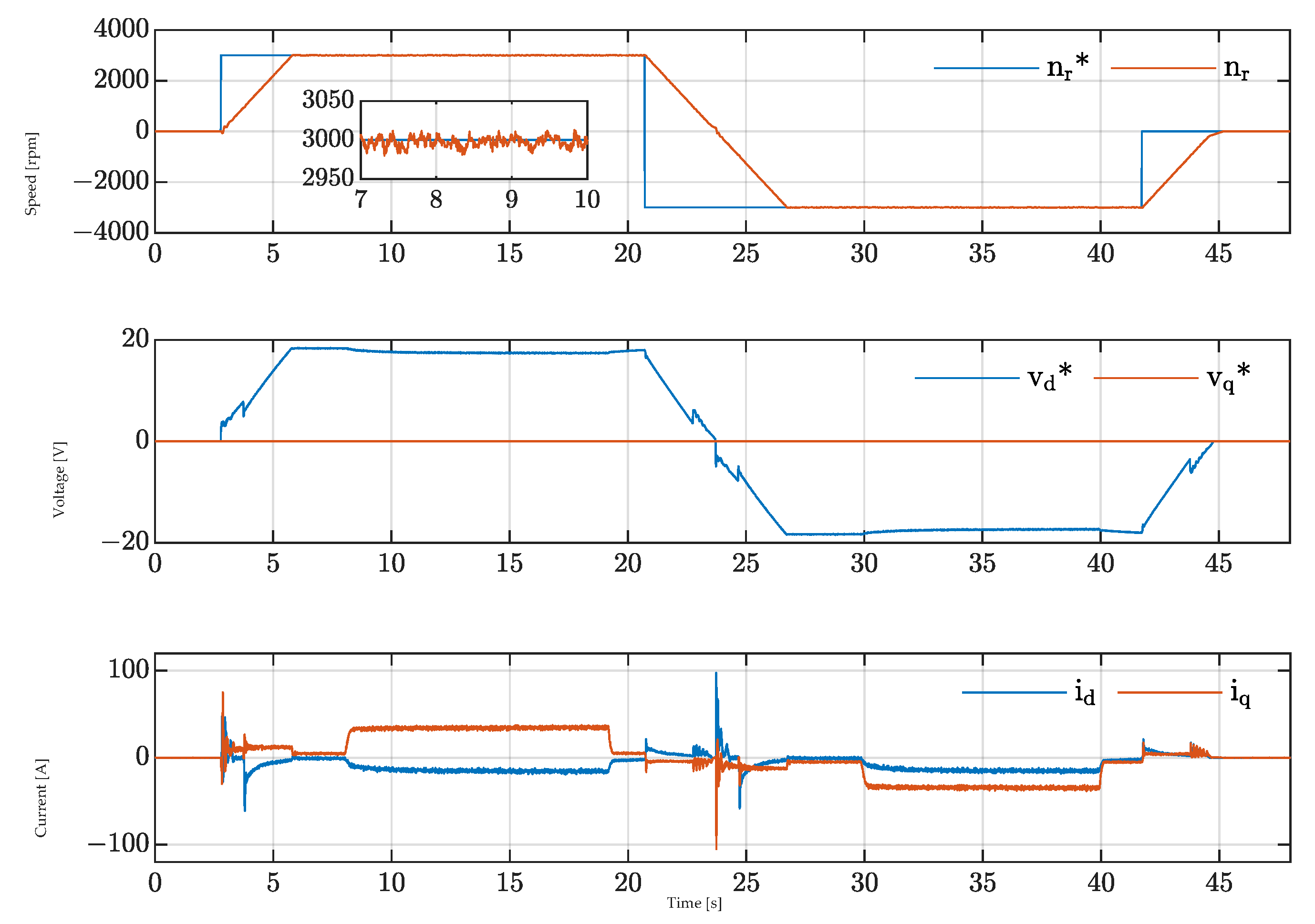
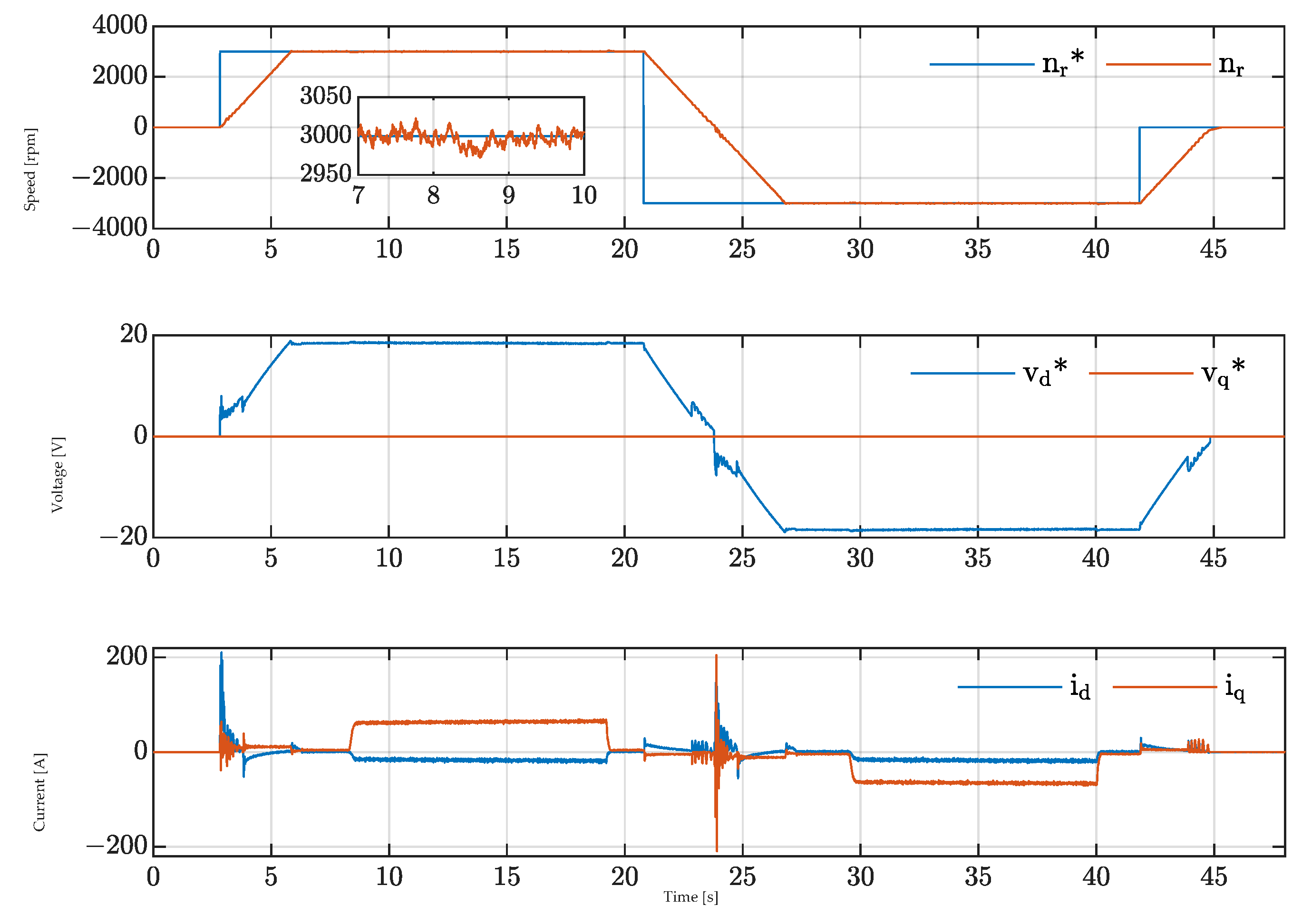
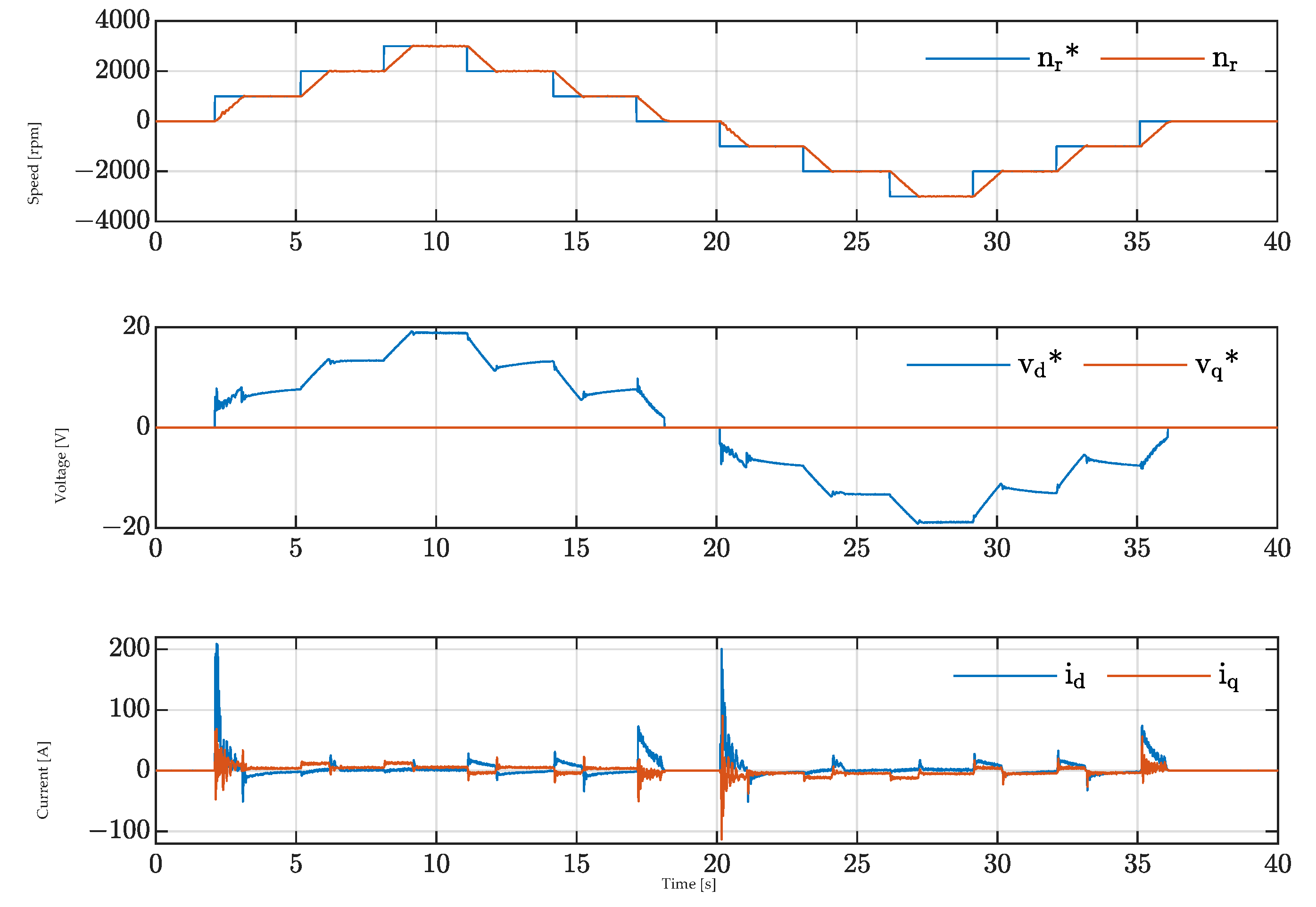
5.2. Experimental Verification of Stable V/f Control with CPF
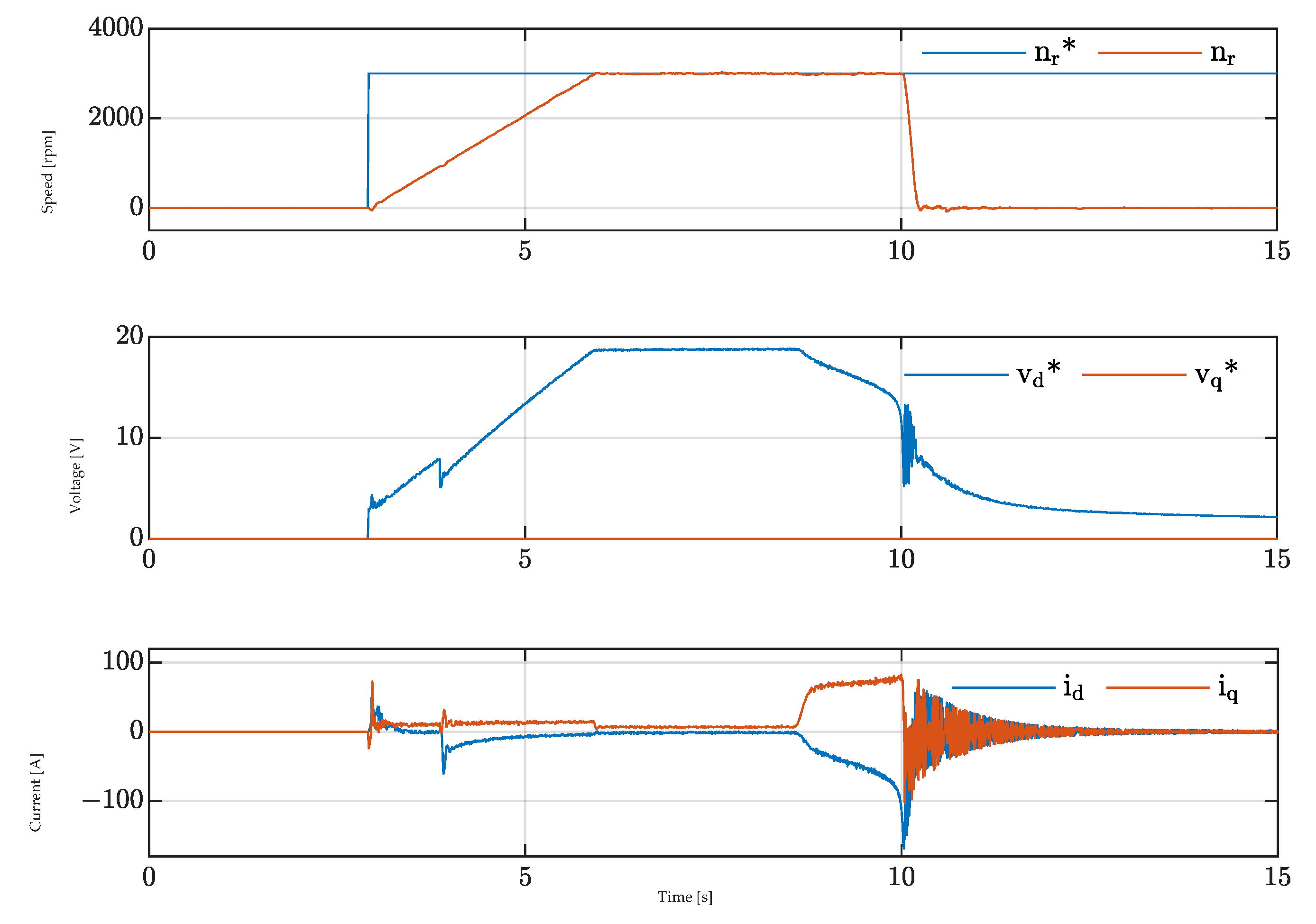
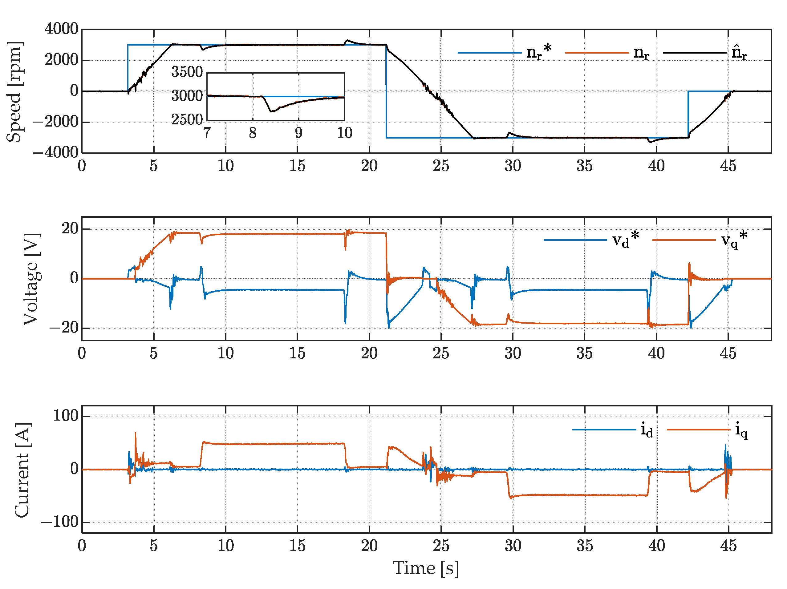
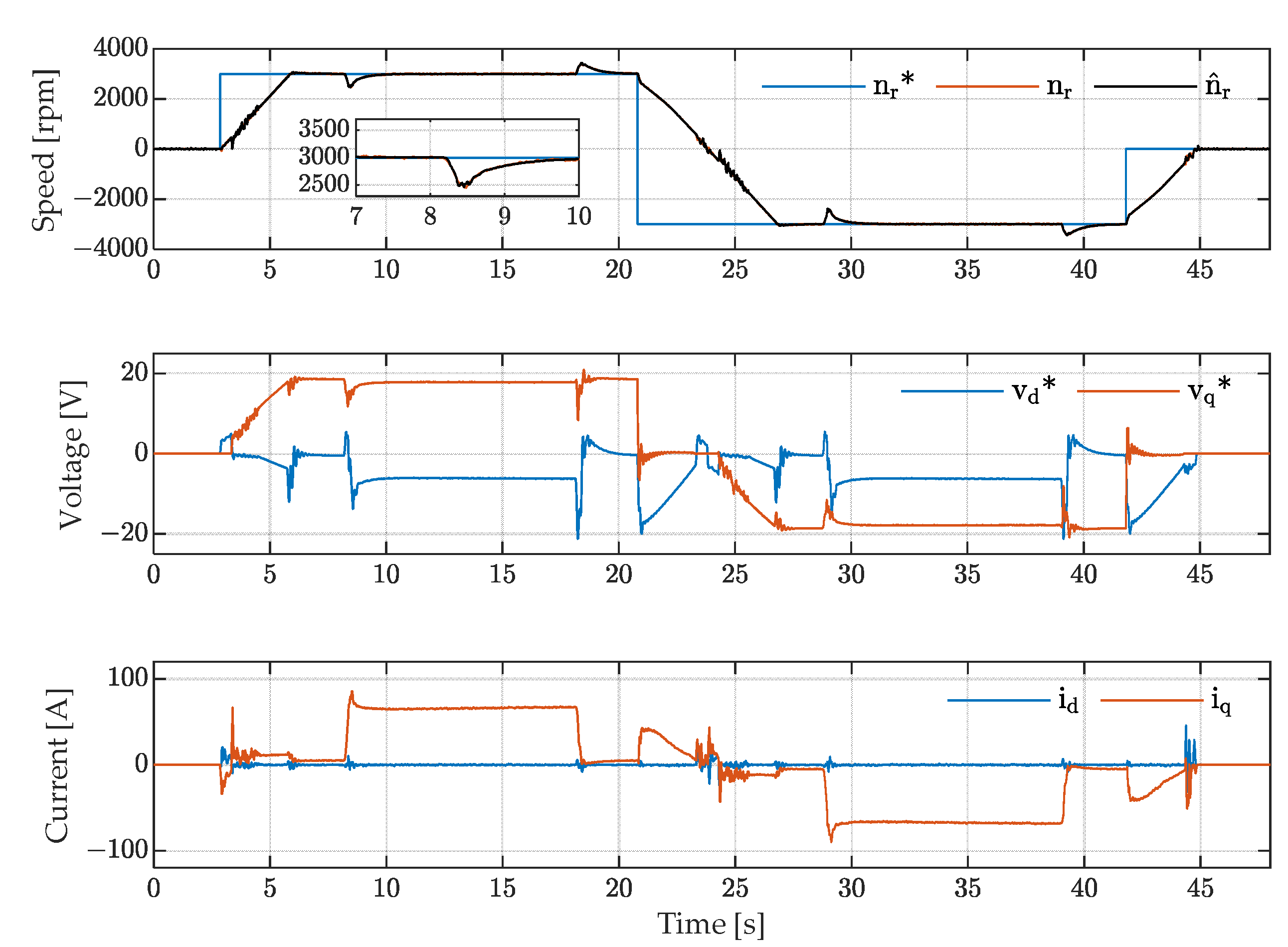
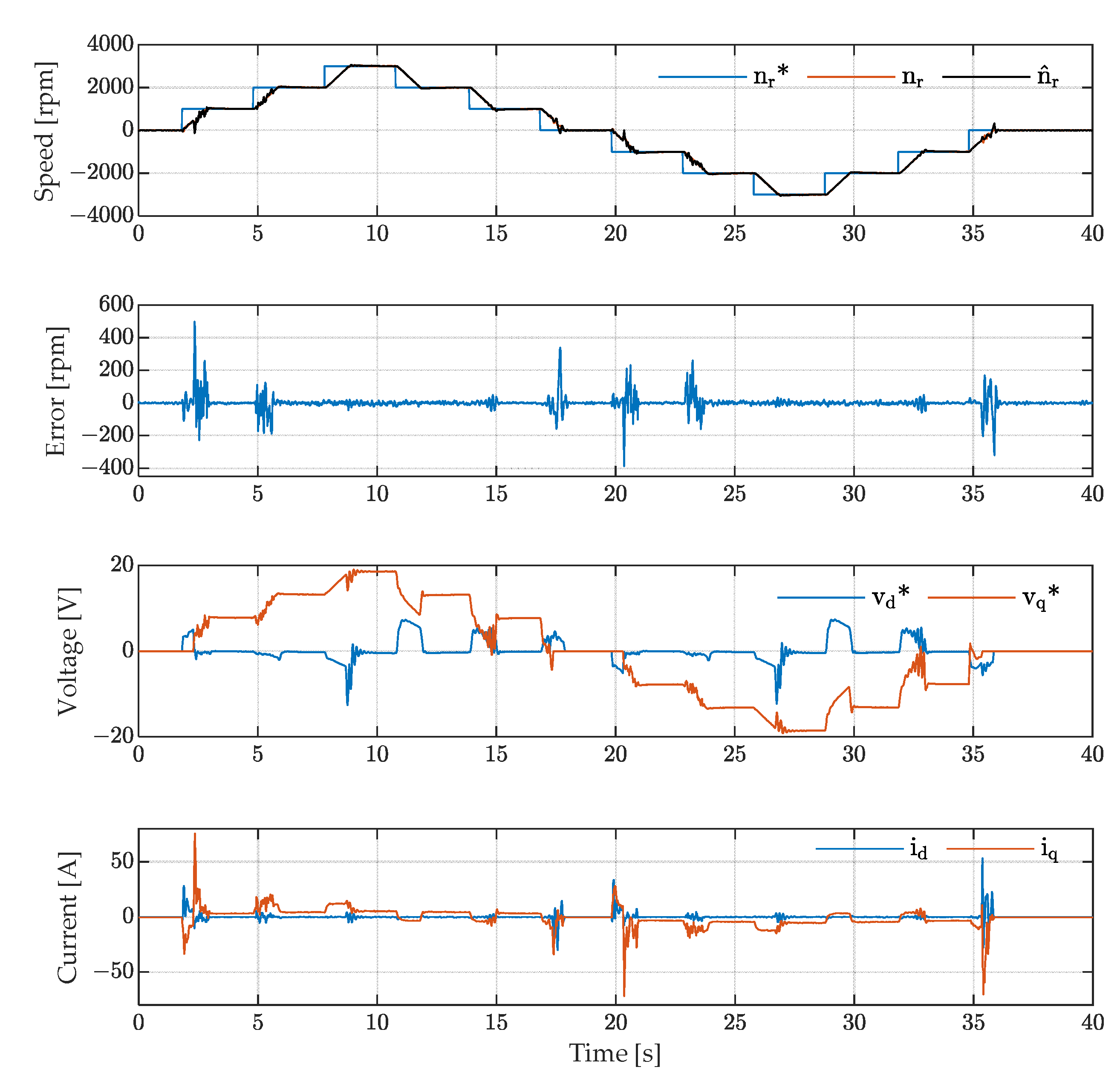
5.3. Experimental Verification of Luenberger-Type Back-EMF Observer in Sensorless FOC
5.4. Comparison of the Main Features for Stable V/f with CPF and Sensorless FOC with Luenberger-Type Back-EMF Observer
6. Conclusions
Author Contributions
Funding
Institutional Review Board Statement
Informed Consent Statement
Data Availability Statement
Conflicts of Interest
Appendix A
| Parameter | Symbol | Value | Unit |
|---|---|---|---|
| Apparent power | 150 | kVA | |
| Nominal voltage | 340 | V | |
| Peak current | 420 | A | |
| PWM switching frequency | 3–12 | kHz | |
| Maximum electrical efficiency | 98 | % |
| Parameter | Symbol | Value | Unit |
|---|---|---|---|
| Rated power | 1.41 | kW | |
| Rated speed | 3000 | rpm | |
| Rated torque | 4.5 | Nm | |
| Rated current | 44.18 | A | |
| Rated frequency | 250 | Hz | |
| Pole pairs | 5 | - | |
| Stator resistance | 0.011 | Ω | |
| d-axis inductance | 0.052 | mH | |
| q-axis inductance | 0.059 | mH | |
| Permanent magnet flux linkage | 0.0108 | Wb | |
| Motor inertia | 5.39 | kg·cm2 | |
| System inertia | 59.5 | kg·cm2 |
| Parameter | Symbol | Value | Unit |
|---|---|---|---|
| Stabilizing loop constant | 20 | - | |
| HPF time constant | 15.9 | ms | |
| Proportional gain of the PI controller in the CPF loop | 0.05 | - | |
| Integral gain of the PI controller in the CPF loop | 1 × 10⁻⁵ | - |
| Parameter | Symbol | Value | Unit |
|---|---|---|---|
| Natural frequency of the speed controller | 0.25 | Hz | |
| Natural frequency of the d-axis and q-axis current controller | 100 | Hz | |
| Natural frequency of the back-EMF observer | 100 | Hz | |
| Natural frequency of the tracking observer | 4 | Hz |
References
- Bolognani, S.; Oboe, R.; Zigliotto, M. Sensorless Full-Digital PMSM Drive with EKF Estimation of Speed and Rotor Position. IEEE Trans. Ind. Electron. 1999, 46, 184–191. [Google Scholar] [CrossRef]
- Wang, Z.; Zheng, Y.; Zou, Z.; Cheng, M. Position Sensorless Control of Interleaved CSI Fed PMSM Drive with Extended Kalman Filter. IEEE Trans. Magn. 2012, 48, 3688–3691. [Google Scholar] [CrossRef]
- Quang, N.K.; Hieu, N.T.; Ha, Q.P. FPGA-Based Sensorless PMSM Speed Control Using Reduced-Order Extended Kalman Filters. IEEE Trans. Ind. Electron. 2014, 61, 6574–6582. [Google Scholar] [CrossRef]
- Orlowska-Kowalska, T.; Dybkowski, M. Stator-Current-Based MRAS Estimator for a Wide Range Speed-Sensorless Induction-Motor Drive. IEEE Trans. Ind. Electron. 2010, 57, 1296–1308. [Google Scholar] [CrossRef]
- Zhu, Y.; Tao, B.; Xiao, M.; Yang, G.; Zhang, X.; Lu, K. Luenberger Position Observer Based on Deadbeat-Current Predictive Control for Sensorless PMSM. Electronics 2020, 9, 1325. [Google Scholar] [CrossRef]
- Chi, S.; Zhang, Z.; Xu, L. Sliding-Mode Sensorless Control of Direct-Drive PM Synchronous Motors for Washing Machine Applications. IEEE Trans. Ind. Appl. 2009, 45, 582–590. [Google Scholar] [CrossRef]
- Kim, H.; Son, J.; Lee, J. A High-Speed Sliding-Mode Observer for the Sensorless Speed Control of a PMSM. IEEE Trans. Ind. Electron. 2011, 58, 4069–4077. [Google Scholar] [CrossRef]
- Rivera Dominguez, J.; Navarrete, A.; Meza, M.A.; Loukianov, A.G.; Canedo, J. Digital Sliding-Mode Sensorless Control for Surface-Mounted PMSM. IEEE Trans. Ind. Inform. 2014, 10, 137–151. [Google Scholar] [CrossRef]
- Song, X.; Fang, J.; Han, B.; Zheng, S. Adaptive Compensation Method for High-Speed Surface PMSM Sensorless Drives of EMF-Based Position Estimation Error. IEEE Trans. Power Electron. 2016, 31, 1438–1449. [Google Scholar] [CrossRef]
- Liang, D.; Li, J.; Qu, R. Sensorless Control of Permanent Magnet Synchronous Machine Based on Second-Order Sliding-Mode Observer with Online Resistance Estimation. IEEE Trans. Ind. Appl. 2017, 53, 3672–3682. [Google Scholar] [CrossRef]
- Wang, Y.; Xu, Y.; Zou, J. Sliding-Mode Sensorless Control of PMSM with Inverter Nonlinearity Compensation. IEEE Trans. Power Electron. 2019, 34, 10206–10220. [Google Scholar] [CrossRef]
- Morimoto, S.; Kawamoto, K.; Sanada, M.; Takeda, Y. Sensorless Control Strategy for Salient-Pole PMSM Based on Extended EMF in Rotating Reference Frame. IEEE Trans. Ind. Appl. 2002, 38, 1054–1061. [Google Scholar] [CrossRef]
- Zhiqian, C.; Tomita, M.; Doki, S.; Okuma, S. An Extended Electromotive Force Model for Sensorless Control of Interior Permanent-Magnet Synchronous Motors. IEEE Trans. Ind. Electron. 2003, 50, 288–295. [Google Scholar] [CrossRef]
- Burgos, R.; Kshirsagar, P.; Lidozzi, A.; Wang, F.; Boroyevich, D. Mathematical Model and Control Design for Sensorless Vector Control of Permanent Magnet Synchronous Machines. In Proceedings of the 2006 IEEE Workshops on Computers in Power Electronics, New York, NY, USA, 16–19 July 2006; pp. 76–82. [Google Scholar]
- Kshirsagar, P.; Burgos, R.P.; Jang, J.; Lidozzi, A.; Wang, F.; Boroyevich, D.; Sul, S.-K. Implementation and Sensorless Vector-Control Design and Tuning Strategy for SMPM Machines in Fan-Type Applications. IEEE Trans. Ind. Appl. 2012, 48, 2402–2413. [Google Scholar] [CrossRef]
- Piippo, A.; Hinkkanen, M.; Luomi, J. Analysis of an Adaptive Observer for Sensorless Control of Interior Permanent Magnet Synchronous Motors. IEEE Trans. Ind. Electron. 2008, 55, 570–576. [Google Scholar] [CrossRef]
- Fatu, M.; Teodorescu, R.; Boldea, I.; Andreescu, G.-D.; Blaabjerg, F. I-F Starting Method with Smooth Transition to EMF Based Motion-Sensorless Vector Control of PM Synchronous Motor/Generator. In Proceedings of the 2008 IEEE Power Electronics Specialists Conference, Rhodes, Greece, 15–19 June 2008; pp. 1481–1487. [Google Scholar]
- Wang, Z.; Lu, K.; Blaabjerg, F. A Simple Startup Strategy Based on Current Regulation for Back-EMF-Based Sensorless Control of PMSM. IEEE Trans. Power Electron. 2012, 27, 3817–3825. [Google Scholar] [CrossRef]
- Wang, M.; Xu, Y.; Zou, J.; Lan, H. An Optimized I-F Startup Method for BEMF-Based Sensorless Control of SPMSM. In Proceedings of the 2017 IEEE Transportation Electrification Conference and Expo, Asia-Pacific (ITEC Asia-Pacific), Harbin, China, 7–10 August 2017; pp. 1–6. [Google Scholar]
- Inoue, Y.; Yamada, K.; Morimoto, S.; Sanada, M. Effectiveness of Voltage Error Compensation and Parameter Identification for Model-Based Sensorless Control of IPMSM. IEEE Trans. Ind. Appl. 2009, 45, 213–221. [Google Scholar] [CrossRef]
- Ichikawa, S.; Tomita, M.; Doki, S.; Okuma, S. Sensorless Control of Synchronous Reluctance Motors Based on Extended EMF Models Considering Magnetic Saturation with Online Parameter Identification. IEEE Trans. Ind. Appl. 2006, 42, 1264–1274. [Google Scholar] [CrossRef]
- Yoo, J.; Lee, Y.; Sul, S.-K. Back-EMF Based Sensorless Control of IPMSM with Enhanced Torque Accuracy Against Parameter Variation. In Proceedings of the 2018 IEEE Energy Conversion Congress and Exposition (ECCE), Portland, OR, USA, 23–27 September 2018; pp. 3463–3469. [Google Scholar]
- Hejny, R.W.; Lorenz, R.D. Evaluating the Practical Low-Speed Limits for Back-EMF Tracking-Based Sensorless Speed Control Using Drive Stiffness as a Key Metric. IEEE Trans. Ind. Appl. 2011, 47, 1337–1343. [Google Scholar] [CrossRef]
- Inoue, Y.; Kawaguchi, Y.; Morimoto, S.; Sanada, M. Performance Improvement of Sensorless IPMSM Drives in a Low-Speed Region Using Online Parameter Identification. IEEE Trans. Ind. Appl. 2011, 47, 798–804. [Google Scholar] [CrossRef]
- Zossak, S.; Sovicka, P.; Sumega, M.; Rafajdus, P. Evaluating Low Speed Limit of Back-EMF Observer for Permanent Magnet Synchronous Motor. Transp. Res. Procedia 2019, 40, 610–615. [Google Scholar] [CrossRef]
- Corley, M.J.; Lorenz, R.D. Rotor Position and Velocity Estimation for a Salient-Pole Permanent Magnet Synchronous Machine at Standstill and High Speeds. IEEE Trans. Ind. Appl. 1998, 34, 784–789. [Google Scholar] [CrossRef]
- Jung-Ik, H.; Ide, K.; Sawa, T.; Sul, S.-K. Sensorless Rotor Position Estimation of an Interior Permanent-Magnet Motor from Initial States. IEEE Trans. Ind. Appl. 2003, 39, 761–767. [Google Scholar] [CrossRef]
- Xie, G.; Lu, K.; Dwivedi, S.K.; Rosholm, J.R.; Blaabjerg, F. Minimum-Voltage Vector Injection Method for Sensorless Control of PMSM for Low-Speed Operations. IEEE Trans. Power Electron. 2016, 31, 1785–1794. [Google Scholar] [CrossRef]
- Kim, S.-I.; Im, J.-H.; Song, E.-Y.; Kim, R.-Y. A New Rotor Position Estimation Method of IPMSM Using All-Pass Filter on High-Frequency Rotating Voltage Signal Injection. IEEE Trans. Ind. Electron. 2016, 63, 6499–6509. [Google Scholar] [CrossRef]
- Ji-Hoon, J.; Sul, S.-K.; Jung-Ik, H.; Ide, K.; Sawamura, M. Sensorless Drive of Surface-Mounted Permanent-Magnet Motor by High-Frequency Signal Injection Based on Magnetic Saliency. IEEE Trans. Ind. Appl. 2003, 39, 1031–1039. [Google Scholar] [CrossRef]
- Shih-Chin, Y.; Lorenz, R.D. Surface Permanent Magnet Synchronous Machine Position Estimation at Low Speed Using Eddy-Current-Reflected Asymmetric Resistance. IEEE Trans. Power Electron. 2012, 27, 2595–2604. [Google Scholar] [CrossRef]
- Yang, S.-C.; Lorenz, R.D. Surface Permanent-Magnet Machine Self-Sensing at Zero and Low Speeds Using Improved Observer for Position, Velocity, and Disturbance Torque Estimation. IEEE Trans. Ind. Appl. 2012, 48, 151–160. [Google Scholar] [CrossRef]
- Seilmeier, M.; Piepenbreier, B. Sensorless Control of PMSM for the Whole Speed Range Using Two-Degree-of-Freedom Current Control and HF Test Current Injection for Low-Speed Range. IEEE Trans. Power Electron. 2015, 30, 4394–4403. [Google Scholar] [CrossRef]
- Young-Doo, Y.; Seung-Ki, S.; Morimoto, S.; Ide, K. High-Bandwidth Sensorless Algorithm for AC Machines Based on Square-Wave-Type Voltage Injection. IEEE Trans. Ind. Appl. 2011, 47, 1361–1370. [Google Scholar] [CrossRef]
- Kim, D.; Kwon, Y.-C.; Sul, S.-K.; Kim, J.-H.; Yu, R.-S. Suppression of Injection Voltage Disturbance for High-Frequency Square-Wave Injection Sensorless Drive with Regulation of Induced High-Frequency Current Ripple. IEEE Trans. Ind. Appl. 2016, 52, 302–312. [Google Scholar] [CrossRef]
- Xu, P.L.; Zhu, Z.Q. Novel Square-Wave Signal Injection Method Using Zero-Sequence Voltage for Sensorless Control of PMSM Drives. IEEE Trans. Ind. Electron. 2016, 63, 7444–7454. [Google Scholar] [CrossRef]
- Ni, R.; Xu, D.; Blaabjerg, F.; Lu, K.; Wang, G.; Zhang, G. Square-Wave Voltage Injection Algorithm for PMSM Position Sensorless Control with High Robustness to Voltage Errors. IEEE Trans. Power Electron. 2017, 32, 5425–5437. [Google Scholar] [CrossRef]
- Wang, G.; Valla, M.; Solsona, J. Position Sensorless Permanent Magnet Synchronous Machine Drives—A Review. IEEE Trans. Ind. Electron. 2020, 67, 5830–5842. [Google Scholar] [CrossRef]
- Hong, J.; Jung, S.; Nam, K. An Incorporation Method of Sensorless Algorithms: Signal Injection and Back EMF Based Methods. In Proceedings of the 2010 International Power Electronics Conference—ECCE ASIA, Sapporo, Japan, 21–24 June 2010; pp. 2743–2747. [Google Scholar]
- Yang, S.-C.; Hsu, Y.-L. Full Speed Region Sensorless Drive of Permanent-Magnet Machine Combining Saliency-Based and Back-EMF-Based Drive. IEEE Trans. Ind. Electron. 2017, 64, 1092–1101. [Google Scholar] [CrossRef]
- Bose, B.K. Control and Estimation of Induction Motor Drives. In Modern Power Electronics and AC Drives; Pearson Education Inc.: Upper Saddle River, NJ, USA, 2002; p. 339. [Google Scholar]
- Perera, P.D.C. Mathematical Models and Control Properties. In Sensorless Control of Permanent-Magnet Synchronous Motor Drives; Aalborg University: Aalborg, Denmark, 2002. [Google Scholar]
- Perera, P.D.C.; Blaabjerg, F.; Pedersen, J.K.; Thogersen, P. A Sensorless, Stable V/f Control Method for Permanent-Magnet Synchronous Motor Drives. IEEE Trans. Ind. Appl. 2003, 39, 783–791. [Google Scholar] [CrossRef]
- Itoh, J.-I.; Nomura, N.; Ohsawa, H. A Comparison between V/f Control and Position-Sensorless Vector Control for the Permanent Magnet Synchronous Motor. In Proceedings of the Power Conversion Conference-Osaka 2002 (Cat. No.02TH8579), Osaka, Japan, 2–5 April 2002; pp. 1310–1315. [Google Scholar]
- Kiuchi, M.; Ohnishi, T.; Hagiwara, H.; Yasuda, Y. V/f Control of Permanent Magnet Synchronous Motors Suitable for Home Appliances by DC-Link Peak Current Control Method. In Proceedings of the 2010 International Power Electronics Conference —ECCE ASIA, Sapporo, Japan, 21–24 June 2010; pp. 567–573. [Google Scholar]
- Sue, S.-M.; Hung, T.-W.; Liaw, J.-H.; Li, Y.-F.; Sun, C.-Y. A New MTPA Control Strategy for Sensorless V/f Controlled PMSM Drives. In Proceedings of the 2011 6th IEEE Conference on Industrial Electronics and Applications, Beijing, China, 21–23 June 2011; pp. 1840–1844. [Google Scholar]
- Kim, W.-J.; Kim, S.-H. A Sensorless V/f Control Technique Based on MTPA Operation for PMSMs. In Proceedings of the 2018 IEEE Energy Conversion Congress and Exposition (ECCE), Portland, OR, USA, 23–27 September 2018; pp. 1716–1721. [Google Scholar]
- Andreescu, G.-D.; Coman, C.-E.; Moldovan, A.; Boldea, I. Stable V/f Control System with Unity Power Factor for PMSM Drives. In Proceedings of the 2012 13th International Conference on Optimization of Electrical and Electronic Equipment (OPTIM), Brasov, Romania, 24–26 May 2012; pp. 432–438. [Google Scholar]
- Coman, C.-E.; Agarlita, S.-C.; Andreescu, G.-D. V/f Control Strategy with Constant Power Factor for SPMSM Drives, with Experiments. In Proceedings of the 2013 IEEE 8th International Symposium on Applied Computational Intelligence and Informatics (SACI), Timisoara, Romania, 23–25 May 2013; pp. 147–151. [Google Scholar]
- Agarlita, S.; Coman, C.; Andreescu, G.; Boldea, I. Stable V/f Control System with Controlled Power Factor Angle for Permanent Magnet Synchronous Motor Drives. IET Electr. Power Appl. 2013, 7, 278–286. [Google Scholar] [CrossRef]
- Isfanuti, A.; Paicu, M.-C.; Andreescu, G.-D.; Tutelea, L.N.; Staudt, T.; Boldea, I. V/f with Stabilizing Loops and MTPA versus Sensorless FOC for PMSM Drives. Electr. Power Compon. Syst. 2020, 48, 1197–1210. [Google Scholar] [CrossRef]
- Vidlak, M.; Gorel, L.; Makys, P. Performance Evaluation, Analysis, and Comparison of the Back-EMF-Based Sensorless FOC and Stable V/f Control for PMSM. In Proceedings of the 2022 International Symposium on Power Electronics, Electrical Drives, Automation and Motion (SPEEDAM), Sorrento, Italy, 22 June 2022; pp. 318–323. [Google Scholar]
- Consoli, A.; Scelba, G.; Scarcella, G.; Cacciato, M. An Effective Energy-Saving Scalar Control for Industrial IPMSM Drives. IEEE Trans. Ind. Electron. 2013, 60, 3658–3669. [Google Scholar] [CrossRef]
- Lee, K.; Han, Y. MTPA Control Strategy Based on Signal Injection for V/f Scalar-Controlled Surface Permanent Magnet Synchronous Machine Drives. IEEE Access 2020, 8, 96036–96044. [Google Scholar] [CrossRef]
- Hrabovcová, V.; Rafajdus, P.; Makyš, P. Analysis of Electrical Machines; IntechOpen: London, UK, 2020; ISBN 978-1-83880-207-3. [Google Scholar]
- Vidlak, M.; Gorel, L.; Makys, P.; Stano, M. Sensorless Speed Control of Brushed DC Motor Based at New Current Ripple Component Signal Processing. Energies 2021, 14, 5359. [Google Scholar] [CrossRef]
- Filka, R.; Balazovic, P.; Dobrucky, B. Transducerless Speed Control with Initial Position Detection for Low Cost PMSM Drives. In Proceedings of the 2008 13th International Power Electronics and Motion Control Conference, Poznan, Poland, 1–3 September 2008; pp. 1402–1408. [Google Scholar]


| Control Structure | PI | I | Park | Clarke | Atan | Filters |
|---|---|---|---|---|---|---|
| Sensorless FOC with the Luenberger-type back-EMF observer | 6 | 1 | 4 | 1 | 1 | 2 |
| Parameter | Stable V/f with CPF | Sensorless FOC with Luenberger-Type Back-EMF Observer |
|---|---|---|
| Accuracy | High | High |
| Dynamics | Good | Very good |
| Parameters dependence | Low | Medium |
| Computational time | Low | High |
| Load disturbance response | Very good | Good |
| Start-up | Good | - |
| Structure tuning | Easy | Hard |
| Low-speed operation | Bad | - |
Publisher’s Note: MDPI stays neutral with regard to jurisdictional claims in published maps and institutional affiliations. |
© 2022 by the authors. Licensee MDPI, Basel, Switzerland. This article is an open access article distributed under the terms and conditions of the Creative Commons Attribution (CC BY) license (https://creativecommons.org/licenses/by/4.0/).
Share and Cite
Vidlak, M.; Makys, P.; Gorel, L. A Novel Constant Power Factor Loop for Stable V/f Control of PMSM in Comparison against Sensorless FOC with Luenberger-Type Back-EMF Observer Verified by Experiments. Appl. Sci. 2022, 12, 9179. https://doi.org/10.3390/app12189179
Vidlak M, Makys P, Gorel L. A Novel Constant Power Factor Loop for Stable V/f Control of PMSM in Comparison against Sensorless FOC with Luenberger-Type Back-EMF Observer Verified by Experiments. Applied Sciences. 2022; 12(18):9179. https://doi.org/10.3390/app12189179
Chicago/Turabian StyleVidlak, Michal, Pavol Makys, and Lukas Gorel. 2022. "A Novel Constant Power Factor Loop for Stable V/f Control of PMSM in Comparison against Sensorless FOC with Luenberger-Type Back-EMF Observer Verified by Experiments" Applied Sciences 12, no. 18: 9179. https://doi.org/10.3390/app12189179