Article

A Generalised Neural Network Model to Estimate Sex from Cranial Metric Traits: A Robust Training and Testing Approach

by
Antonietta Del Bove
1,2 and
Alessio Veneziano
3,*
1
Departament d’Historia i Història de l’Art, Universitat Rovira i Virgili, Avinguda de Catalunya 35, 43002 Tarragona, Spain
2
Institut Català de Paleoecologia Humana i Evolució Social (IPHES-CERCA), Edifici W3, Campus Sescelades URV, Zona Educational 4, 43007 Tarragona, Spain
3
Department of Archaeology, University of Cambridge, Downing Street, Cambridge CB2 3DZ, UK
*
Author to whom correspondence should be addressed.
Appl. Sci. 2022, 12(18), 9285; https://doi.org/10.3390/app12189285
Submission received: 29 June 2022 / Revised: 7 September 2022 / Accepted: 10 September 2022 / Published: 16 September 2022

Abstract

:

Featured Application

The method presented can be used to estimate sex attributes from a small set of cranial metric traits.

Abstract

The morphology of the human cranium allows for reconstructing important information about the identity of an individual, such as age, ancestry, sex, and health status. The estimation of sex from morphology is a key component of the work of physical anthropologists, and in the last decade, the field has witnessed an increase in the use of novel algorithm-based methodologies to tackle the aforementioned task. Nevertheless, several limitations (e.g., small training/testing sample size, training-test data relatedness, limited population inclusiveness, overfitting) have hampered the application of such methods as a standardised procedure in the field. Here, we propose a population-inclusive protocol for estimating sex from a small set of cranial metric traits (10 measurements) based on a neural network architecture trained to maximise the probability of sex attribution and prevent overfitting. The cross-validation returned an accuracy of 86.7% ± 0.02% and log loss of 0.34 ± 0.03. The protocol developed was tested on data unrelated to that of the training and validation phase and returned an estimated accuracy of 84.3% and log loss of 0.348. The model and the related code to use it are made publicly available.

1. Introduction

One fundamental task of physical anthropologists is that of reconstructing the biological identity of human remains from the incomplete information provided by the skeleton or parts of it [1]. Available methods to establish the sex from the skeleton include protocols based on the visual inspection of morphological traits differing between males and females or quantitative methods often relying on linear measurements used to discriminate between sexes by means of specific algorithms. Such methods have been successfully applied to attribute sex from several different elements within the human skeleton (i.e., femur [2], humerus [3], pelvis [4], teeth [5], talus and calcaneus [6], upper limb [7], and the metacarpal bones [8]). To achieve the highest accuracy, the analysis of the most dimorphic skeletal regions is desirable, such as the coxal bone and other post-cranial elements [9]; when these are not available, another useful source of information is found in the cranium [1,10]. Some important sources of information regarding sexual dimorphism in the human cranium reside in the occipital protuberance, the mastoid process, and the glabellar region [11,12], among others. To provide a standardised approach, potentially less prone to individual bias, it is essential to refine the quantitative methodologies currently available, defining their limitations and establishing the expected performance achievable. In traditional anthropology, a common procedure for estimating sex from the cranium uses a scoring system of morphological traits evaluated visually [11,13]. Despite being a straightforward and practical method, the success of these traditional approaches depends directly on the experience of the observer, and errors due to subjectivity tend to be higher than in quantitative methods [14,15]. To overcome such obstacles, the use of quantitative measurements and algorithm-based methods have received considerable attention in the last decades.
Previous studies have highlighted the challenges of extrapolating sex information from cranial morphology and variability. The cranium, by its own nature, is a sum of multivariate factors, such as ontogeny, ageing, diet, genetics, epigenetics, and pathologies [16], and it is, therefore, difficult to isolate sex-related information from those confounding factors. Another great challenge comes from the relationship between morphology and ancestry. For example, some studies define small and gracile skulls as females, while the attributes of a large size and robust appearance are associated with males [12,17,18]. These differences cannot be applied to humans tout court because the association between the robust/gracile appearance is never perfectly binary: depending on the population, it is possible to find small males and robust females and overlapping morphological variability between sexes is common in modern humans [16], as it is the general overlapping among populations [19]. These circumstances led several authors to focus their studies on individual populations [20,21,22,23,24], which produce results that can hardly be extrapolated to the whole human variability.
The last few decades have witnessed a remarkable development in quantitative methods such as geometric morphometrics and machine learning, which have been successfully applied to Biological and Forensic Anthropology [25,26,27]. Those methods have triggered a tremendous growth in the search for new quantitative solutions to the problem of estimating sex from the human skeleton [19,28,29,30,31]. In particular, machine learning (ML) provides a flexible approach to estimating attributes such as sex from skeletal measurements—an approach adopted more and more in the field [25,26,27,28,29,30,31,32].
All too often, though, algorithm-based studies addressing sex estimation from the human cranium suffer from a lack of “generalisability” and the absence of a solid testing framework. Part of the issue derives from the use of only limited human variability, for example, during the training phase of the ML applications: as mentioned above, studies on individual populations, or groups of populations, have been prioritised [29,32,33], probably because of the difficulty of accessing worldwide data of known sex [34]. Furthermore, testing is often performed on samples too small to provide statistical reliance [35,36,37], and those samples are often part of the same body of data (e.g., collected by the same observer, belonging to the same population/group) used during the training phase [38], which potentially limits the population-inclusive application of the estimation achieved.
The shortcomings of previous approaches are not only limited to the source and size of the sample. The number of variables considered can be problematic for several reasons. Cranial variables can be highly correlated with each other because of morphological integration [24], and this can make the dataset redundant. The more the number of variables, the higher the redundancy, which increases the risk of overfitting (i.e., when the prediction performs well on the training data but cannot generalise on unseen data [39]). Furthermore, the use of several variables can become problematic when dealing with incomplete cranial remains, a common occurrence with archaeological and forensic material.
An additional limitation is the over-reliance on “accuracy” as a measure of performance. The accuracy of an estimation reflects the proportion of cases correctly assigned to their class: in a binary situation, such as the estimation of sex, the accuracy is computed by counting how many males and females are identified as males or females, respectively. Quantitative algorithms, though, provide the estimation in terms of probability, and, in a binary case, observation is attributed to a class if it has a probability higher than 0.5 for that class, although the threshold can be different. Therefore, accuracy does not account for the probability of the estimation (its “strength”, in other words) because the same result is obtained regardless of whether the probability of an observation being male or female is 0.51 or 0.99. The usefulness of accuracy is dependent on where we set the cut-off probability [40].
The result of the abovementioned limitations is that, as of today, we lack a clear understanding of the potential of quantitative applications for the estimation of sex from the human cranium. In fact, although previous applications have fuelled research on the subject, the training and testing frameworks they used were prone to potential bias to an extent difficult to pinpoint, thus limiting their use as standardised methods for estimating sex. Here, we try to overcome those limitations using a population-inclusive neural network approach based on large training and testing datasets from different sources, requiring a limited number of traits and maximising the probability of estimation rather than accuracy. The advances produced by this work are three-fold: (I) it provides an estimation easy to transfer to other datasets, regardless of ancestry; (II) it clarifies the potential of quantitative, algorithm-based estimation of sex from human crania, maximising probability over accuracy; (III) it presents a step-by-step protocol for the application of ML-based predictions to solve basic problems in the field of physical anthropology.

2. Materials and Methods

2.1. The Datasets

Machine learning applications make use of three sets of data, namely Training, Validating, and Testing. The training set is used to provide the algorithm with “learning material”, on which it iteratively improves its performance to build an optimal model; the performance during training is assessed on the validating set; finally, the testing set is an external source of data for evaluating the ability of the model to generalise its performance. This work relies on two sources of cranial measurements: Howell’s craniometric dataset [41,42,43] and the University of Tennessee (UT) Database for Forensic Anthropology in the United States [44]. Here, Howell’s data is used during the training and validation steps, while the UT Forensic dataset is used for testing. Howell’s dataset consists of 82 craniometric measurements recorded on 2524 human crania from 30 populations with worldwide distribution. The UT Database for Forensic Anthropology includes 36 craniomandibular variables recorded on 1396 individuals of mixed ancestry (identified or unidentified) from forensic cases (from 1962 to 1991) in the United States.

2.2. Data Preparation

Ten craniometric measurements were selected from the datasets, and their definitions are reported in Table 1. The measurements were chosen to represent most of the morphology of the human cranium using only a reduced number of variables (to reduce redundancy across measurements); at the same time, the measurements were chosen to account for some cranial traits previously associated with high levels of sexual dimorphism in modern humans (e.g., mastoid and orbital shape [1,45,46]. The measurements are shown in Figure 1. Only adult individuals were included in the analysis. The sex attribution in Howell’s dataset is not known with certainty but is estimated based on non-metric traits by the same William Howell, using a procedure described in [43]. Although it is not ideal to train the model on specimens whose sex is estimated, this choice was necessary due to the difficulties of finding cranial metric datasets of suitable size and with worldwide representation; therefore, this limitation may be reflected in the final model. To balance population representation within the dataset, we removed populations including only one or the other sex. In the UT database, sex information is based on direct identification or on soft tissue estimation—only individuals whose sex is identified directly are included in our dataset—thus, the sex of the individuals included in this dataset is known. To avoid biases during the training and testing phases, in both datasets, the female and male sample size was balanced by randomly reducing the male subsample (originally more abundant).
To account for outliers in Howell’s dataset, all the observations that exceed three standard deviations from the mean of at least one of the 10 measurements were removed. Outliers were not removed from the UT dataset because it constitutes the test data and because of the need for evaluating the performance of the eventual model on a realistic variability of the human cranium. Missing data were present in the subset obtained for the UT dataset; those individuals missing 50% of data or more (at least 5 out of 10 measurements) were discarded from the dataset. The other incomplete observations were estimated using Additive Regression, performed using the R package “Hmisc” [47]. The percentage of missing data in each measurement did not exceed 7.9%. In both datasets, the 10 linear measurements were adjusted for the isometric effect of size using Mosimann transformation, which weighs each measurement on the geometric mean of all measurements [48]. The geometric mean was included as an additional measurement in both datasets to explicitly represent size. The measurements were then standardised by z-score transformation (scaled to zero mean and unit variance).
The transformed measurements are henceforth referred to as features, in line with the current use in machine learning applications. The final size of Howell’s dataset is 2292 individuals, including 1146 females and 1146 males; the final UT dataset consists of 606 individuals, 303 females and 303 males. Each dataset includes 11 metric features generated from 10 measurements. Specifics of the sample are also reported in Table 2.

2.3. The Classification Algorithm

The Machine Learning application presented here is a classification task, with the ultimate target of finding a model capable of attributing sex based on a limited number of metric cranial features. The steps followed in the procedure described below are summarised in Figure 2. The implementation of the classification task was performed using the open-source Machine Learning platform “H2O” through the R interface package “h2o” [49].
The sex-classification model was implemented using a feedforward neural network [50], consisting of an input layer (that introduces the features into the network), one or more hidden layers (that transform the input features), and an output layer (the last layer that receives the data processed within the network and produces a result). Each layer is made of nodes (also called neurons or perceptrons), which are the network’s computational units. Every time an input travels to a node of the hidden layers, it is multiplied by some weight, which modifies the influence of that input on the output. At each node of the hidden layers, multiple weighted input features arrive and are combined by an activation function, whose output is a new input to another hidden layer or to the output layer. In this work, we use a non-linear activation function (see Table 3) to allow the output model to identify non-linear patterns in the differences between females and males.

2.4. Parameter Tuning

Machine Learning algorithms operate depending on certain fundamental hyperparameters (henceforth just parameters), whose values govern the way the algorithm performs. To find a suitable model, the initial step is to find the combination of parameter values that provide the best performance for the generated model—an operation referred to as “parameter tuning” [39,51]. Here, parameter tuning was performed using a “brute force” approach (also known as “grid search”) by training the algorithm multiple times, each with different combinations of the parameters, and then validating the performance of the models thus generated.
The neural network algorithm depends on several parameters, and the most important ones account for the network’s architecture and are the number of hidden layers and the number of nodes per layer; the larger these values, the more complex the output model can be, and this can allow more subtle differences to be identified. Nevertheless, model complexity can lead to overfitting when the model learns to classify the data in the training set but has poor predictive abilities on new data [39]. Overfitting is particularly common in applications using limited amounts of observations, such as this work and several applications in the archaeological and anthropological fields, where data are often scarce. A limited number of features (a characteristic of our dataset) can help lower the chance of overfitting by reducing redundant information [52]—this is the case when using cranial measurements because they are correlated with each other. To further reduce the chance of overfitting, regularisation parameters can be tuned. Regularisation is a set of techniques used to avoid overfitting by reducing complexity through the penalisation of the features’ influence [39]. In the case of a Neural Network, regularisation can assign zero to part of the weights (L1-regularisation), or it can make those weights smaller (L2-regularisation).
The training was tuned over two values for the number of hidden layers (1 and 2) and over seven values for the number of nodes (3, 7, 11, 15, 19, 23, and 27—the same number of nodes was used in all hidden layers). Additionally, a sequence of seven values for the L2-regularisation parameter (0, 1 × 10⁻⁴, 5 × 10⁻⁴, 1 × 10⁻³, 5 × 10⁻³, 1 × 10⁻² and 5 × 10⁻²) was used in the tuning. The overall number of different models trained during the tuning phase was 98 (2 × 7 × 7). The values of other parameters (see Table 3) were estimated using a trial-and-error manual tuning, thus reducing the computational time needed for the “brute force” approach.

2.5. Training and Validation

Training and validation were performed for each model for a set number of epochs. Each epoch can be seen as a learning cycle: at each epoch, the training data are fed to the input layer, they get weighed along the path to the hidden layers, and a predictive model is returned through the output layer. A prediction is then performed on the validation data and compared to the observed output (in our case, the observed sex of the individuals in the validation set) to evaluate the performance of the current model. In the next epoch, the weights are modified to improve the model performance according to the result in the previous epoch. The performance can be evaluated based on different metrics [53].
In this work, the training and validation data were obtained from Howell’s dataset using 10-fold cross-validation; therefore, each of the 98 models was trained 10 times, with approximately 90% of the data used for training and 10% for validating the model performance. The data were assigned to each fold using a stratified approach [54] to ensure balanced sex classes within the folds.
The model performance is here evaluated on the validation set using the log loss metric (or cross-entropy). Since the model assigns a probability of being female or male to any new observation, we want to obtain a model whose prediction yields the highest possible probability of belonging to a given class. The log loss metric measures how close the predicted probability is to certainty (probability of 1); the smaller the divergence, the lower the log loss [55]. Ideally, we want log loss to approach zero, but for a balanced binary classification task, a realistic and useful upper-threshold value is set at 0.693—this is the non-informative log loss, or the value of log loss when both classes are predicted with probability equal to 0.5 (same probability of assigning an observation to the female or male class). The training is therefore performed by reducing log loss along the epochs.
Here, training and validation are performed for a maximum of 1000 epochs. To reduce the computational time, we used an early-stopping technique, which stops the training process when the performance does not change over a specified tolerance for a specified number of cycles [56]. In the present case, training is set to stop when log loss stays within a tolerance of 1 × 10⁻⁴ for 20 consecutive cycles. Therefore, training does not usually run for the maximum number of epochs allowed. Values of log loss below 0.693 indicate that the fitted model performs better than a random prediction.

2.6. Best Model, Variable Importance, and Testing

All the models generated during tuning (trained and validated) are scouted for the model with the best performance, which is evaluated based on the prediction of each model on the validation set. After the best-performing model is detected, the final model is built, which is the ultimate output of the training procedure. The final training is carried out on a compound dataset including both training and validation data (joined into a single training set), and the parameters are assigned the values that those same parameters have in the best-performing model of the tuning phase. When the final model is obtained, its ability to generalise its predictive power is evaluated on the test set.
Here, the best-performing among the 98 models of the tuning phase was chosen based on multiple factors. First, the best model is the one whose prediction on the validation set returned the lowest log loss; this ensures that the final model is capable of attributing sex with the highest per-class probability. Second, we wanted to maximise the area under the receiver operating characteristic (ROC) curve, a quantity also known as area under curve (AUC). The ROC is a probability curve comparing the false positive rate (FPR or 1-specificity) and true positive rate (TPR or sensitivity) of a binary outcome when the cut-off probability for deciding whether to assign an observation to a certain class is lowered sequentially from one to zero. Therefore, AUC measures how well the model distinguishes both classes of a binary outcome in a way that is independent of the cut-off chosen for the class attribution [53]. Finally, when different models have similar log loss and AUC, the models with lower complexity are chosen; in our case, we gave preference to models with only one layer and a low number of nodes to reduce the chances of overfitting.
When the best-performing model was chosen, the final model was trained on the whole Howell’s dataset using the values of the parameters shown in Table 3, as we did during the tuning phase, with the exception of the tuned parameters, whose values were those found via parameter tuning. The relative importance of each feature in the model was computed in the “h2o” R package following the method of Gedeon [57]. The final model was then used to predict the known sex of the observations in the test set, to assess its performance on data not included in the training phase and, therefore, unseen by the model. The model and code to use it are made publicly available on GitHub (github.com/AlessioVeneziano/Papers/tree/main/DelBove_%26_Veneziano_2022, accessed on 9 September 2022).

3. Results

3.1. Best Model Selection

The results of parameter tuning for the 98 models evaluated showed an improvement in performance with an increasing number of nodes and decreasing L2 regularisation (Figure 3). log loss was consistently lower than the non-informative threshold (0.693 for a binary classification), reaching the lowest value of 0.339 at 27 nodes and L2 parameter equal to 5 × 10⁻³, when one hidden layer was used, and of 0.346 with 19 nodes, L2 equal to zero and two hidden layers. Log loss was consistently lower for models using one hidden layer rather than two, although the differences were small for models with more than 11 nodes and low L2 parameter. AUC was always higher in models with one hidden layer and less variable among models (Figure 3), suggesting that two hidden layers may introduce a degree of overfitting in the conditions analysed here. The highest AUC of 0.929 was obtained with one hidden layer, 11 nodes, and L2 equal to 1 × 10⁻⁴.
To choose the best model, we accounted for both log loss and AUC, also prioritising the least complex model to avoid overfitting. We picked the best performing model among those trained with one hidden layer because they consistently outperformed models with two hidden layers. Among those models, the lowest log loss and highest AUC were obtained with different parameter values, as reported above: 27 nodes and L2 of 5 × 10⁻³, and 11 nodes and L2 of 1 × 10⁻⁴, respectively. The performance of those two models differed negligibly: the difference in AUC and log loss was 5 × 10⁻⁴ and 2 × 10⁻³, respectively. Based on these results, we can confidently prioritise the least complex model among the ones performing best for AUC and log loss. The selected model had one hidden layer, 11 nodes, and L2 equal to 1 × 10⁻⁴.
The model chosen as the best performing (based on the criteria stated above) was among the models with the lowest log loss and highest AUC among those validated in the present study (Figure 4). The performance on cross-validation returned an accuracy of 0.867 ± 0.022, AUC of 0.929 ± 0.017, and log loss of 0.341 ± 0.033. Furthermore, when we look at the learning curves for the best model (Figure 5), we can appreciate how the performance (log loss and AUC) of the training and validation sets had a comparable pattern and small difference, reaching a point of stability along the epochs. The pattern shown in Figure 5 suggests that the model selected had not undergone overfitting.

3.2. Variable Importance and Model Performance

The estimation of the relative feature importance (Figure 6) shows that the model’s prediction was highly influenced by the geometric mean computed on the other measurements (GM: 19.7%), which includes size, followed by the bizygomatic breadth (ZYB: 14.4%) and mastoid height (MDH: 10.2%). The remaining features had smaller contributions (each less than 10%), with the lowest scores shown by basion-bregma height and nasal height (BBH and NLH: 4.7%).
When the performance was assessed on the 606 individuals (303 females, 303 males) of the test dataset, 266 out of 303 females were correctly sexed by the model, and 245 out of 303 for the male group. The model estimated sex with an accuracy of 0.843, and the intra-group accuracy was 0.809 for females and 0.878 for males, thus indicating a better performance for the male group. The log loss estimated on the test set performance was 0.348, much lower than the uninformative threshold of 0.693, suggesting that the observations are estimated with probabilities generally higher than 0.5. Figure 7 shows the histogram of the estimated probabilities of being female/male for the observations whose sex was correctly identified by the model. Ideally, we want the distribution to be negatively skewed (larger frequency of high probabilities); such a pattern was observed for our test sample, with 90% of the correctly sexed observations being estimated with a probability equal or higher than 0.66 (female) and 0.70 (male). The distribution of estimated probabilities for males was particularly skewed, with more than 40% of correctly sexed observations estimated with a probability equal or higher than 0.98.
The AUC of an ROC curve is a better estimator of performance than accuracy when we deal with binary classification. In fact, AUC provides an indication of the performance of both classes through a single metric. The ROC curve of the model prediction is shown in Figure 8. The AUC measured on the test set was 0.923.

4. Discussion

The literature regarding sex estimation from the human cranium is abundant and has flourished through the use of algorithm-based approaches. Nevertheless, generalising previous findings is tricky because of the focus limited to single populations, but also because the results from such approaches can be misleading if testing is not performed accurately (e.g., using statistically-relevant sample sizes, checking model overfitting, adopting representative performance metrics). Here, we addressed some of those issues by training a neural network on a limited set of cranial measurements from a broad human variability and generating a model independent of ancestry and robust to overfitting. The model was tested on unseen data of known sex, and its performance was evaluated using a probability-based metric (log loss).

4.1. The Model Performance

Our model uses only 10 linear measurements (Table 1) to describe cranial shape, with the addition of the geometric mean computed from those measurements. The best performing model (established based on parameter tuning on cross-validated data) was able to estimate sex with 84% accuracy. This result is virtually free of overfitting (see methods for information about how it was avoided), and the log loss performance shows that 90% of the individuals attributed to the correct sex were estimated with a probability higher than 0.65 (Figure 7). Our findings suggest that the model generated is capable of working efficiently with only a limited number of measurements (a positive characteristic for applications on fragmentary crania). Although this result appears underwhelming if compared to the higher accuracies reached by other studies [28,58], it must be highlighted that those studies have tested data on only small datasets, which cannot guarantee protection from random sampling effects. In this study, the model was tested on more than 600 individuals, suggesting that the result observed here is more reliable. Furthermore, here we base the evaluation of model performance on log loss, which accounts for the probability of the estimation—this is not common practice in the literature regarding sex estimation from skeletal material, and the absence of such information makes it difficult to assess the performance of previous models.
The model generated here was built on a broad cranial variability of modern H. sapiens, which suggests an easier generalisability to applications beyond single populations, although this was not explicitly tested. In addition, the accuracy demonstrated is remarkable if we consider that the training dataset consists of crania whose sex was estimated using a visual approach [41,42,43]. This finding is relevant because large datasets of known sex are very rare and often difficult to access, and sex estimation through visual inspection approaches can introduce biases, especially with regard to size [14,58]. By monitoring the model performance through metrics such as AUC, it is possible to check for the prevalence of correct estimations for both sexes. In fact, AUC can account simultaneously for the classification of both classes in a binary application [59] (Figure 8). In this study, AUC was taken into account when tuning the parameters to choose the best-performing model among those generated. Thanks to the protocol used and based on the performance observed during testing, we can confidently assume that the model is unbiased toward one or the other sex.

4.2. The Variable Importance

The measurements used to build the neural network model were purposely chosen to represent as much cranial variability as possible by keeping only the essential amount of morphological information. Those choices aim to increase the chances of application (e.g., when crania are only fragmentary) but also to reduce the chances of overfitting. In choosing the measurements to include in the dataset, we also made sure to include traits that were previously recognised as sexually dimorphic in modern humans. How the variables are allowed to interact in the model is hard to pinpoint; in fact, neural networks and other algorithms are referred to as “black boxes” [60]. This means that the way in which the model is classifying the crania (e.g., the nature and degree of interaction across the metric traits used) is not straightforward (especially because we used a non-linear activation function). Nevertheless, we can make assumptions regarding the model based on the measured variable importance, which represents an approximation of the influence of each trait on the estimation.
The variable deemed to be the most relevant in the estimation was the geometric mean (Figure 6). This variable was computed from the 10 metric traits to represent the size of the cranium. Size was virtually erased from the other measurements thanks to the Mosimann transformation [48]; thus, we can expect that the sexual differences in overall dimensions were gathered in this single feature. The observed importance of geometric mean suggests that size is an important aspect of human cranial dimorphism, although it must be highlighted that, in the model, size may have been interacting with other features; thus, it could be important only in association with other sources of morphological variability.
Following size, the second most important feature was the bizygomatic breadth, followed by mastoid height and biauricular height (Figure 6). Bizygomatic breadth was analysed in several studies [17,22,61,62,63,64], and in each, bizygomatic breadth measurement positively discriminated sex. Moreover, in other studies using different approaches than the one adopted here, the shape of zygomatic arches resulted in a diagnosis of sex [14,65].
Mastoid height was formerly known to vary between sexes [42,65]. Mastoid bones are more developed in males than in females, and thus, the mastoid influence on our model is not a surprise (see Figure 6). Third in importance in our model was the biauricular breadth, lesser known than the bizygomatic breadth for its sex-related differences, but previously reported in the literature [17,61,64].
All measurements selected for our model are noted in the literature [17,22,61,62,63,64,66], except for the orbital height. This measurement is not considered sexually dimorphic by various authors [17,61,64]; however, it presented a non-negligible influence on our model. This result is in agreement with the use of orbital shapes for sexing individuals through visual inspection [41,59]. Finally, the nasal region seems to contribute to a minor degree to the sexual dimorphism of the human cranium, which could support the idea that the morphology of the nasal area is functionally determined [60].

5. Conclusions

In this work, we attempted to overcome some of the common methodological obstacles encountered when estimating sex from cranial measurements using an algorithm-based approach. Some limitations are still present, such as the model training with crania, whose sex was estimated, a necessary decision (see Section 2.2). Nevertheless, the model generated is a step forward in the establishment of standardised procedures for the semi-automated estimation of individual attributes from skeletal material. The trained neural network model is made publicly available on GitHub with no restrictions (github.com/AlessioVeneziano/Papers/tree/main/DelBove_%26_Veneziano_2022, accessed on 9 September 2022). We also describe the protocol of model training, validating, and testing in detail to allow reproducibility and correct usage of machine learning applications in the field of physical anthropology. The findings presented here provide evidence regarding the extent to which cranial metric traits can be used for attributing sex to skeletal material and highlight the potential that machine learning methods have to automate sex estimation from the crania.

Author Contributions

Conceptualisation, A.D.B. and A.V.; methodology, A.D.B. and A.V.; software, A.V.; validation, A.V.; formal analysis, A.D.B. and A.V.; investigation, A.D.B. and A.V.; resources, A.V.; data curation, A.D.B. and A.V.; writing—original draft preparation, A.D.B.; writing—review and editing, A.D.B. and A.V.; visualisation, A.D.B. and A.V.; supervision, A.V.; project administration, A.V. All authors have read and agreed to the published version of the manuscript.

Funding

A.D.B. is funded by the Martí i Franquès fellowship programme (number 2020pmf-pipf-43); A.V. was not supported by external fundings for this work.

Institutional Review Board Statement

The study uses publicly available datasets and did not make physical use of human material. No Ethical Approval was needed or this study.

Informed Consent Statement

The study does not include or disclose personal information that could allow the identification of human individuals, living or dead.

Data Availability Statement

Howell’s craniometric dataset is publicly available at https://web.utk.edu/~auerbach/HOWL.htm (accessed on 1 April 2022) by Benjamin M. Auerbach, PhD; the Database for Forensic Anthropology at the University of Tennessee (UT) is distributed by the National Archive of Criminal Justice Data (NACJD) at https://doi.org/10.3886/ICPSR02581.v1. The code to reproduce the analysis, the model generated, and the script to use the model are made publicly available on GitHub at the following link: https://github.com/AlessioVeneziano/Papers/tree/main/DelBove_%26_Veneziano_2022 (accessed on 1 April 2022). The data from the UT Database for Forensic Anthropology cannot be provided by third parties; thus, it is not included in the GitHub source.

Acknowledgments

We want to express our gratitude to Carlos Lorenzo and Antonio Profico for their invaluable insights and inputs provided during the preparation of this work.

Conflicts of Interest

The authors declare no conflict of interest.

References

  1. Bass, W.M.; Folkens, P.A. Human Osteology in a Laboratory and Field Manual of the Human Skeleton; Gulf Professional Publishing: Houston, TX, USA, 1995. [Google Scholar]
  2. Seidemann, R.M.; Stojanowski, C.M.; Doran, G.H. The use of the supero-inferior femoral neck diameter as a sex assessor. Am. J. Phys. Anthropol. 1998, 107, 305–313. [Google Scholar] [CrossRef]
  3. López-Lázaro, S.; Pérez-Fernández, A.; Alemán, I.; Viciano, J. Sex estimation of the humerus: A geometric morphometric analysis in an adult sample. Leg. Med. 2020, 47, 101773. [Google Scholar] [CrossRef] [PubMed]
  4. Phenice, T.W. A newly developed visual method of sexing the os pubis. Am. J. Phys. Anthropol. 1969, 30, 297–302. [Google Scholar] [CrossRef] [PubMed]
  5. García-Campos, C.; Martinón-Torres, M.; De Pinillos, M.M.; Modesto-Mata, M.; Martín-Francés, L.; Perea-Pérez, B.; Zanolli, C.; De Castro, J.M.B. Modern humans sex estimation through dental tissue patterns of maxillary canines. Am. J. Phys. Anthropol. 2018, 167, 914–923. [Google Scholar] [CrossRef]
  6. Curate, F.; d’Oliveira Coelho, J.; Silva, A.M. CalcTalus: An online decision support system for the estimation of sex with the calcaneus and talus. Archaeol. Anthropol. Sci. 2021, 13, 73. [Google Scholar] [CrossRef]
  7. Bidmos, M.A.; Mazengenya, P. Accuracies of discriminant function equations for sex estimation using long bones of upper extremities. Int. J. Legal. Med. 2021, 135, 1095–1102. [Google Scholar] [CrossRef]
  8. Barrio, P.A.; Trancho, G.J.; Sánchez, J.A. Metacarpal sexual determination in a Spanish population. J. Forensic Sci. 2006, 51, 990–995. [Google Scholar] [CrossRef]
  9. Spradley, M.K.; Jantz, R.L. Sex estimation in forensic anthropology: Skull versus postcranial elements. J. Forensic Sci. 2011, 56, 289–296. [Google Scholar] [CrossRef]
  10. Byers, S.N. Introduction to Forensic Anthropology; Routledge: Boston, MA, USA, 2002. [Google Scholar]
  11. Acsádi, G.; Nemeskéri, J. History of Human Life Span and Mortality. Available online: https://scholar.google.es/scholar?hl=it&as_sdt=0%2C5&q=acsadi+and+nemeskeri+1970&oq=ascadi+ (accessed on 17 March 2019).
  12. Buikstra, J.; Ubelaker, D. Standards for Data Collection from Human Skeletal Remains: Proceedings of a Seminar at the Field Museum of Natural History Arkansas Archaeology, Fayetteville Arkansas Archaeological Survey. Available online: http://scholar.google.com/scholar?hl=en&btnG=Search&q=intitle:Standards+for+Data+Collection+from+Human+Skeletal+Remains+Proceedings+of+a+Seminar+at+the+Field+Museum+of+Natural+History#0 (accessed on 17 March 2019).
  13. Walker, P.L. Sexing skulls using discriminant function analysis of visually assessed traits. Am. J. Phys. Anthropol. 2008, 136, 39–50. [Google Scholar] [CrossRef]
  14. Walrath, D.E.; Turner, P.; Bruzek, J. Reliability test of the visual assessment of cranial traits for sex determination. Am. J. Phys. Anthropol. 2004, 125, 132–137. [Google Scholar] [CrossRef]
  15. Williams, B.A.; Rogers, T.L. Evaluating the accuracy and precision of cranial morphological traits for sex determination. J. Forensic Sci. 2006, 51, 729–735. [Google Scholar] [CrossRef] [PubMed]
  16. Klales, A.R. Sex Estimation of the Human Skeleton; Academic Press: Cambridge, MA, USA, 2020. [Google Scholar] [CrossRef]
  17. Franklin, D.; Freedman, L.; Milne, N. Sexual dimorphism and discriminant function sexing in indigenous South African crania. HOMO-J. Comp. Hum. Biol. 2005, 55, 213–228. [Google Scholar] [CrossRef]
  18. Weiss, K.M. On the systematic bias in skeletal sexing. Am. J. Phys. Anthropol. 1972, 37, 239–249. [Google Scholar] [CrossRef] [PubMed]
  19. Garvin, H.M.; Ruff, C.B. Sexual dimorphism in skeletal browridge and chin morphologies determined using a new quantitative method. Am. J. Phys. Anthropol. 2012, 147, 661–670. [Google Scholar] [CrossRef] [PubMed]
  20. Franklin, D.; Oxnard, C.E.; O’Higgins, P.; Dadour, I. Sexual dimorphism in the subadult mandible: Quantification using geometric morphometrics. J. Forensic Sci. 2007, 52, 6–10. [Google Scholar] [CrossRef]
  21. Boucherie, A.; Chapman, T.; García-Martínez, D.; Polet, C.; Vercauteren, M. Exploring sexual dimorphism of human occipital and temporal bones through geometric morphometrics in an identified Western-European sample. Am. J. Biol. Anthropol. 2022, 178, 54–68. [Google Scholar] [CrossRef]
  22. Dayal, M.R.; Spocter, M.A.; Bidmos, M.A. An assessment of sex using the skull of black South Africans by discriminant function analysis. HOMO-J. Comp. Hum. Biol. 2008, 59, 209–221. [Google Scholar] [CrossRef]
  23. Green, H.; Curnoe, D. Sexual dimorphism in Southeast Asian crania: A geometric morphometric approach. HOMO-J. Comp. Hum. Biol. 2009, 60, 517–534. [Google Scholar] [CrossRef]
  24. Milella, M.; Franklin, D.; Belcastro, M.G.; Cardini, A. Sexual differences in human cranial morphology: Is one sex more variable or one region more dimorphic? Anat. Rec. 2021, 304, 2789–2810. [Google Scholar] [CrossRef]
  25. Attia, M.H.; Kholief, M.A.; Zaghloul, N.M.; Kružić, I.; Anđelinović, Š.; Bašić, Ž.; Jerković, I. Efficiency of the adjusted binary classification (ABC) approach in osteometric sex estimation: A comparative study of different linear machine learning algorithms and training sample sizes. Biology 2022, 11, 917. [Google Scholar] [CrossRef]
  26. Nikita, E.; Nikitas, P. On the use of machine learning algorithms in forensic anthropology. Leg. Med. 2020, 47, 101771. [Google Scholar] [CrossRef] [PubMed]
  27. Savall, F.; Faruch-Bilfeld, M.; Dedouit, F.; Sans, N.; Rousseau, H.; Rougé, D.; Telmon, N. Metric sex determination of the human coxal bone on a virtual sample using decision trees. J. Forensic Sci. 2015, 60, 1395–1400. [Google Scholar] [CrossRef] [PubMed]
  28. Bewes, J.; Low, A.; Morphett, A.; Pate, F.D.; Henneberg, M. Artificial intelligence for sex determination of skeletal remains: Application of a deep learning artificial neural network to human skulls. J. Forensic Leg. Med. 2019, 62, 40–43. Available online: https://www.sciencedirect.com/science/article/pii/S1752928X18304219 (accessed on 9 April 2021). [CrossRef] [PubMed]
  29. Imaizumi, K.; Bermejo, E.; Taniguchi, K.; Ogawa, Y.; Nagata, T.; Kaga, K.; Hayakawa, H.; Shiotani, S. Development of a sex estimation method for skulls using machine learning on three-dimensional shapes of skulls and skull parts. Forensic Imaging 2020, 22, 200393. [Google Scholar] [CrossRef]
  30. Chovalopoulou, M.-E.; Valakos, E.; Manolis, S.K. Sex determination by three-dimensional geometric morphometrics of craniofacial form. Anthr. Anz. 2016, 73, 195–206. [Google Scholar] [CrossRef] [PubMed]
  31. Jurda, M.; Urbanová, P. Sex and ancestry assessment of Brazilian crania using semi-automatic mesh processing tools. Leg. Med. 2016, 23, 34–43. [Google Scholar] [CrossRef]
  32. Kelley, S.R.; Tallman, S.D. Population-Inclusive Assigned-Sex-at-Birth Estimation from Skull Computed Tomography Scans. Forensic Sci. 2022, 2, 321–348. [Google Scholar] [CrossRef]
  33. Milella, M.; Belcastro, M.G.; Zollikofer, C.P.; Mariotti, V. The effect of age, sex, and physical activity on entheseal morphology in a contemporary Italian skeletal collection. Am. J. Phys. Anthr. 2012, 148, 379–388. [Google Scholar] [CrossRef]
  34. Ortega, R.F.; Irurita, J.; Campo, E.J.E.; Mesejo, P. Analysis of the performance of machine learning and deep learning methods for sex estimation of infant individuals from the analysis of 2D images of the ilium. Int. J. Leg. Med. 2021, 135, 2659–2666. [Google Scholar] [CrossRef]
  35. Toneva, D.; Nikolova, S.; Agre, G.; Zlatareva, D.; Hadjidekov, V.; Lazarov, N. Machine learning approaches for sex estimation using cranial measurements. Int. J. Legal Med. 2021, 135, 951–966. [Google Scholar] [CrossRef]
  36. Navega, D.; Vicente, R.; Vieira, D.N.; Ross, A.H.; Cunha, E. Sex estimation from the tarsal bones in a Portuguese sample: A machine learning approach. Int. J. Leg. Med. 2015, 129, 651–659. [Google Scholar] [CrossRef] [PubMed]
  37. Ortiz, A.G.; Costa, C.; Silva, R.; Biazevic, M.; Michel-Crosato, E. Sex estimation: Anatomical references on panoramic radiographs using Machine Learning. Forensic Imaging 2020, 20, 200356. [Google Scholar] [CrossRef]
  38. Curate, F.; Umbelino, C.; Perinha, A.; Nogueira, C.; Silva, A.M.; Cunha, E. Sex determination from the femur in Portuguese populations with classical and machine-learning classifiers. J. Forensic Leg. Med. 2017, 52, 75–81. [Google Scholar] [CrossRef]
  39. Ying, X. An Overview of Overfitting and its Solutions. J. Phys. Conf. Ser. 2019, 1168, 022022. [Google Scholar] [CrossRef]
  40. Jerković, I.; Bašić, Ž.; Anđelinović, Š.; Kružić, I. Adjusting posterior probabilities to meet predefined accuracy criteria: A proposal for a novel approach to osteometric sex estimation. Forensic Sci. Int. 2020, 311, 110273. [Google Scholar] [CrossRef] [PubMed]
  41. Howells, W.W. Who’s who in skulls. Ethnic identification of crania from measurements. Pap. Peabody Mus. Archaeol. Ethnol. 1995, 82, 108. [Google Scholar]
  42. Howells, W.W. Skull shapes and the map. Craniometric analyses in the dispersion of modern homo. Pap. Peabody Mus. Archaeol. Ethnol. 1989, 79, 189. [Google Scholar]
  43. Howells, W.W. Cranial variation in man. A study by multivariate analysis of patterns of differences among recent human populations. Pap. Peabody Mus. Archeol. Ethnol. 1973, 67, 259. [Google Scholar]
  44. Jantz, R.L.; Moore-Jansen, P.H. A Data Base for Forensic Anthropology; The National Institute of Justice: Washington, DC, USA, 1988.
  45. Holland, T.D. Sex determination of fragmentary crania by analysis of the cranial base. Am. J. Phys. Anthr. 1986, 70, 203–208. [Google Scholar] [CrossRef]
  46. Saini, V.; Srivastava, R.; Rai, R.K.; Shamal, S.N.; Singh, T.B.; Tripathi, S.K. Sex Estimation from the Mastoid Process Among North Indians. J. Forensic Sci. 2011, 57, 434–439. [Google Scholar] [CrossRef]
  47. Harrell, F.E.; Dupont, C. Hmisc. Harrell Miscellaneous; CRAN: Brisbane, Australia, 2022. [Google Scholar]
  48. Mosimann, J.E. Size Allometry: Size and Shape Variables with Characterizations of the Lognormal and Generalized Gamma Distributions. J. Am. Stat. Assoc. 1970, 65, 930–945. [Google Scholar] [CrossRef]
  49. LeDell, E.; Gill, N.; Aiello, S.; Fu, A.; Candel, A.; Click, C.; Kraljevic, T.; Nykodym, T.; Aboyoun, P.; Kurka, M.; et al. R Interface for the ‘H2O’ Scalable Machine Learning Platform; CRAN: Brisbane, Australia, 2022. [Google Scholar]
  50. Svozil, D.; Kvasnieka, V.; Pospichal, J. Chemometrics and intelligent laboratory systems Introduction to multi-layer feed-forward neural networks. Chemom. Intell. Lab. Syst. 1997, 39, 43–62. [Google Scholar] [CrossRef]
  51. Lavesson, N.; Davidsson, P. Quantifying the Impact of Learning Algorithm Parameter Tuning. In Proceedings of the National Conference on Artificial Intelligence, Boston, MA, USA, 16–20 July 2006; Volume 1. [Google Scholar]
  52. Venkatesh, B.; Anuradha, J. A Review of Feature Selection and Its Methods. Cybern. Inf. Technol. 2019, 19, 3–26. [Google Scholar] [CrossRef]
  53. Erickson, B.J.; Kitamura, F. Magician’s Corner: 9. Performance Metrics for Machine Learning Models. Radiol. Artif. Intell. 2021, 3, e200126. [Google Scholar] [CrossRef] [PubMed]
  54. Parsons, V.L. Stratified sampling. In Wiley StatsRef: Statistics Reference Online; Wiley: Hoboken, NJ, USA, 2014; pp. 1–11. [Google Scholar]
  55. Cybenko, G.; O’Leary, D.P.; Rissanen, J. The Mathematics of Information Coding, Extraction and Distribution; Springer Science & Business Media: Berlin, Germany, 1998; Volume 107. [Google Scholar]
  56. Caruana, R.; Lawrence, S.; Giles, C. Overfitting in neural nets: Backpropagation, conjugate gradient, and early stopping. Adv. Neural. Inf. Process. Syst. 2000, 13, 381–387. [Google Scholar]
  57. Gedeon, T.D. Data Mining of Inputs: Analysing Magnitude and Functional Measures. Int. J. Neural Syst. 1997, 8, 209–218. [Google Scholar] [CrossRef]
  58. Gao, H.; Geng, G.; Yang, W. Sex determination of 3D skull based on a novel unsupervised learning method. Comput. Math. Methods Med. 2018, 2018, 4567267. [Google Scholar] [CrossRef]
  59. Kubat, M.; Matwin, S. Addressing the curse of imbalanced training sets: One-sided selection. Icml 1997, 97, 179. [Google Scholar]
  60. McClelland, J.L.; Rumelhart, D.E.; PDP Research Group. Parallel Distributed Processing, Volume 2: Explorations in the Microstructure of Cognition: Psychological and Biological Models; MIT Press: Cambridge, MA, USA, 1987; Volumes 1 & 2. [Google Scholar]
  61. Ramamoorthy, B.; Pai, M.M.; Prabhu, L.V.; Muralimanju, B.; Rai, R. Assessment of craniometric traits in South Indian dry skulls for sex determination. J. Forensic Leg. Med. 2016, 37, 8–14. [Google Scholar] [CrossRef]
  62. Saini, V.; Srivastava, R.; Rai, R.K.; Shamal, S.N.; Singh, T.B.; Tripathi, S.K. An Osteometric Study of Northern Indian Populations for Sexual Dimorphism in Craniofacial Region. J. Forensic Sci. 2011, 56, 700–705. [Google Scholar] [CrossRef]
  63. Kranioti, E.F.; Apostol, M.A. Sexual dimorphism of the tibia in contemporary Greeks, Italians, and Spanish: Forensic implications. Int. J. Legal. Med. 2015, 129, 357–363. [Google Scholar] [CrossRef] [PubMed]
  64. Cappella, A.; Gibelli, D.; Vitale, A.; Zago, M.; Dolci, C.; Sforza, C.; Cattaneo, C. Preliminary study on sexual dimorphism of metric traits of cranium and mandible in a modern Italian skeletal population and review of population literature. Leg. Med. 2020, 44, 101695. [Google Scholar] [CrossRef] [PubMed]
  65. Garvin, H.M.; Sholts, S.B.; Mosca, L.A. Sexual dimorphism in human cranial trait scores: Effects of population, age, and body size. Am. J. Phys. Anthropol. 2014, 154, 259–269. [Google Scholar] [CrossRef] [PubMed]
  66. Ekizoglu, O.; Hocaoglu, E.; Inci, E.; Can, I.O.; Solmaz, D.; Aksoy, S.; Buran, C.F.; Sayin, I. Assessment of sex in a modern Turkish population using cranial anthropometric parameters. Leg. Med. 2016, 21, 45–52. [Google Scholar] [CrossRef] [PubMed]
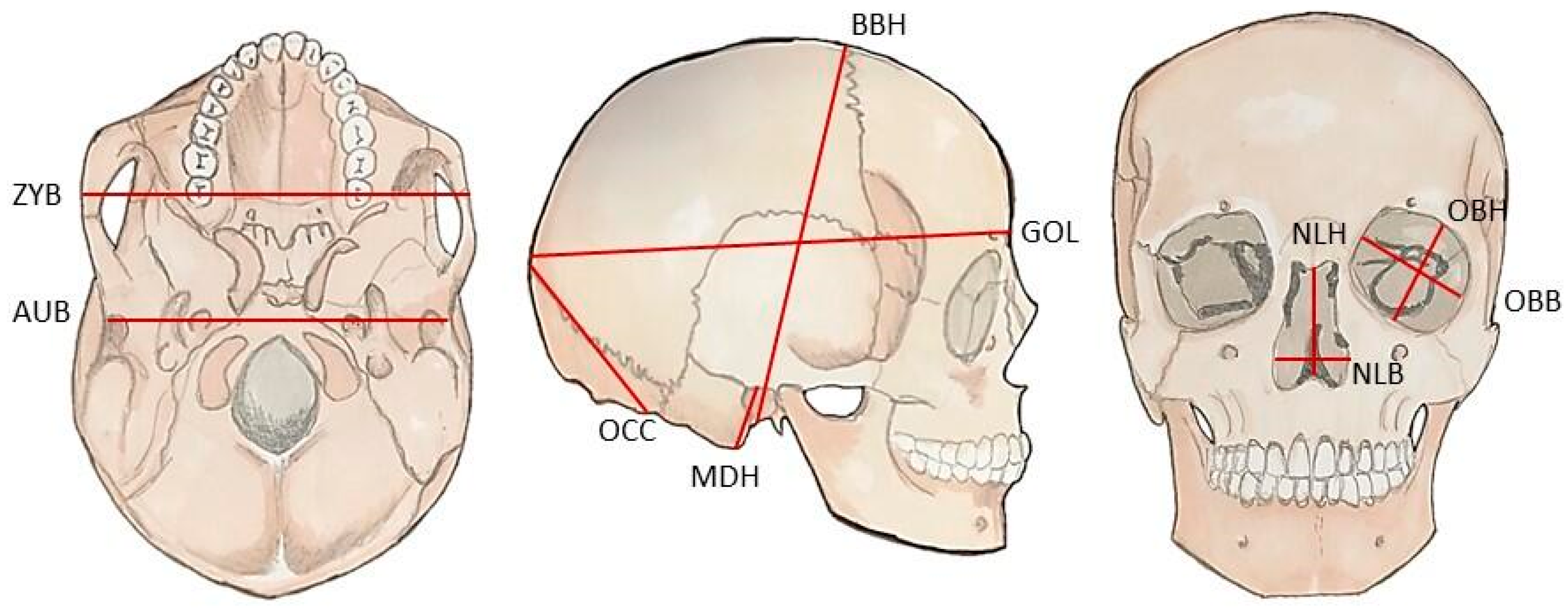
Figure 1. Graphical representation of the 10 cranial measurements used in the analysis. The measurements respect the anthropological standard established by Howells [36]. Definitions are provided in Table 1. (ZYB: bizygomatic breadth; MDH: mastoid height; AUB: biauricular breadth; OBH: orbit height; GOL: glabella-occipital length; NLB: nasal breadth; OCC: lambda-opisthion chord; OBB: orbit breadth; BBH: basion-bregma height; NLH: nasal height).
Applsci 12 09285 g001
Figure 2. Schematic representation of the machine learning workflow adopted. The data for the parameter tuning were divided into 10 sets of training and validation datasets, allowing cross-validation of the models evaluated and then fed to the neural network algorithm. The algorithm returns the performance of the models on the validation sets, which is the basis for selecting the tuned parameters that allowed best performance for the model. The model is trained on a joint dataset (train + validation) to obtain the best performing model. The performance of the best model is assessed using a test dataset, unseen during the previous phases of the workflow.
Applsci 12 09285 g002
Figure 3. Performance of the sex classification on the validation dataset during parameter tuning. The top graphs show the performance as log loss, while the bottom ones use the area under the receiver operating characteristic (ROC) curve (area under curve or AUC). The performance is compared across different values of the tuned parameters: L2 regularisation, number of nodes per layer, and number of hidden layers (the results for models trained with one hidden layer are shown on the left, with two hidden layers on the right). The performance improves from yellow to blue, specifically with log loss decreasing and AUC increasing. The blue sphere indicates the best performing model: it shows the maximum performance obtained and the relative values of the tuned parameters that produce that performance.
Applsci 12 09285 g003
Figure 4. Percentage distribution of the performance metrics—log loss and area under curve (AUC)—across all models trained and validated during parameter tuning. The dashed vertical lines indicate the performance of the best model selected (left: log loss; right: AUC).
Applsci 12 09285 g004
Figure 5. Learning curves showing performance of classification during the epochs. Performance is shown as log loss and area under curve (AUC), measured on the training and validation datasets (in darker and lighter colours, respectively). The similar pattern measured for the two datasets suggests that the performance learned through the training set was generalised to the validation set, thus indicating no overfitting occurred.
Applsci 12 09285 g005
Figure 6. Relative importance of each feature in the best model selected. The importance is shown as a percentage. (GM: geometric mean; ZYB: bizygomatic breadth; MDH: mastoid height; AUB: biauricular breadth; OBH: orbit height; GOL: glabella-occipital length; NLB: nasal breadth; OCC: lambda-opisthion chord; OBB: orbit breadth; BBH: basion-bregma height; NLH: nasal height).
Applsci 12 09285 g006
Figure 7. Distribution of the probabilities returned by the best model for correctly estimated females (orange) and males (blue). The dashed vertical lines show the first decile of probability, which indicates the probability above which 90% of observations are estimated.
Applsci 12 09285 g007
Figure 8. Receiver operating characteristic (ROC) curve showing the observed performance (compared to the uninformative case—random prediction—and a perfect estimation, where all observations were correctly assigned to their true class.
Applsci 12 09285 g008
Table 1. Cranial measurements used in the analysis, abbreviations, and definitions.
MeasurementAbbreviationDefinition
Biauricular breadthAUBThe shortest distance across the roots of the zygomatic processes
Basion-bregma heightBBHThe linear distance from basion to bregma
Glabella-occipital lengthGOLThe linear distance from glabella to opisthocranion along the midsagittal plane
Mastoid heightMDHThe linear distance between porion and mastoidale points
Nasal breadthNLBThe maximum breadth of the nasal aperture
Nasal heightNLHThe height from the nasion to the lowest point on the rim of the nasal aperture
Orbit breadthOBBThe linear distance from dacryon to ectoconchion points
Orbit heightOBHThe linear distance between the superior and inferior margins of the orbits, measured perpendicularly to orbital breadth
Lambda-opisthion chordOCCThe linear distance from lambda to opisthion along the mid-sagittal plane
Bizygomatic breadthZYBThe maximum breadth across the zygomatic arches, perpendicular to the mid-sagittal plane
Table 2. Details of the sample used. Source, population (if known), and sex attribution are reported. Sample sizes refer to the datasets after the transformations operated for the scopes of the current study.
DatasetSourcePopulationSex (F:M)
Training and ValidationWilliam W. Howell’s
craniometric dataset
Ainu38:46
Andaman31:33
Arikara27:36
Atayal17:26
Australia (aboriginals)49:50
Berg53:53
Buriat54:45
Bushman46:39
Dogon51:45
Easter Island37:42
Egypt (600–200 B.C.)53:53
Eskimo55:43
Guam27:28
Hainan38:43
Mokapu49:45
Moriori51:54
Japan (North)32:52
Japan (South)41:45
Norse (medieval)54:52
Peru55:49
Santa Cruz51:47
Tasmania (aboriginals)42:40
Teita50:32
Tolai54:49
Zalavar (medieval)45:49
Zulu46:50
TestUniversity of Tennessee
Database for Forensic
Anthropology in the
United States
Ancestry unknown303:303
Table 3. Crucial parameters of the neural network algorithm, definitions, and values adopted.
ParameterValue *
Epochs1000
Stopping metricLog loss
Loss functionCross entropy
DistributionBernoulli
Learning rate5 × 10−4
Momentum start0.5
Momentum ramp1 × 10−6
Momentum stable0.99
Stopping rounds20
Stopping tolerance1 × 10−4
Input dropout ratio0
Number of folds10
Fold assignmentStratified
Activation functionRectifier with dropout
L1 regularisation0
L2 regularisation0, 1 × 10⁻⁴, 5 × 10⁻⁴, 1 × 10⁻³, 5 × 10⁻³, 1 × 10⁻², and 5 × 10⁻²
Hidden layers1 and 2
Nodes per layer3, 7, 11, 15, 19, 23, and 27
* The values used for the parameters refer to the options set in the h2o.deeplearning function in the “h2o” R package [51]. Parameters not shown are left as default as per version 3.36.0.3 of the “h2o” package. When multiple values are shown, the parameter underwent tuning via the brute force approach.
Publisher’s Note: MDPI stays neutral with regard to jurisdictional claims in published maps and institutional affiliations.

