Calibration and Testing of Discrete Element Simulation Parameters for Sandy Soils in Potato Growing Areas

Abstract

To improve the accuracy of discrete element simulation in the process of separating potato–soil mixtures, the contact parameters of sandy soil with 3, 6, 9, and 12% water content were calibrated in DEM simulation using EDEM software simulation. The error of the rest angle between them was used as an index, and the approach of performing only one simulation and multiple Box–Behnken response surface analyses was proposed to determine the optimal parameter combinations. Meanwhile, unconfined compression and direct shear tests were conducted to obtain the parameters of polymer bonds for soil with different water content, and a simulation was carried out using EDEM. The test results show that the significant parameters affecting the rest angle are JKR surface energy, soil interparticle recovery coefficient, and rolling friction factor. The numerical simulation of the rest angle was compared with the physical test, and the maximum relative error between them was 4.72%. The bond parameters of soil with different water content and firmness were obtained and compared with the simulation test, the maximum error was 6.53% for the direct shear test and 8.07% for the unconfined compression test, which proved that the bonding parameters are reliable and provide an effective parametric and theoretical basis for the discrete element simulation of soil particles.

1. Introduction

In the context of the national potato as a staple food strategy, the scale of potato cultivation in China has increased [1] and the demand for mechanized potato harvesting has increased accordingly, and the potato–soil separation stage effect is one of the important criteria to measure the performance of harvesting machines. Nowadays, oscillating separation screens are widely used in potato harvesters because of their simple structure and high efficiency in potato–soil separation. However, the current research on oscillating sieves mainly focuses on reducing potato damage and improving the rate of bright potatoes, while little research has been reported on the crushing characteristics of the soil during separation. In the process of potato–soil separation, soil crushing and potato skin damage are contradictory: the more significant the soil crushing, the more serious the potato damage. Therefore, it is necessary to analyze soil crushing characteristics in order to obtain reasonable parameters for the oscillating sieve, so that potato–soil separation is maximized and potato damage is reduced.

The analysis of soil forces and motion in the actual harvesting process is too complex, and there are many limitations in conducting experiments, making it difficult to conduct in-depth research. In 1971, the discrete element method (DEM) was first applied by Cundall. Nowadays, DEM is widely used in agriculture [2]. It provides a new method to investigate soil motion and fragmentation characteristics and can simulate the actual working conditions and visually reflect the soil motion and force situation, which is conducive to efficient and convenient analysis. However, due to the diversity of soil types, the physical parameters of soil in different regions are very different. In order to ensure the accuracy of the parameters used in the simulation model, the physical parameters of the soil need to be calibrated.

In the discrete element simulation, density, Poisson’s ratio, elastic modulus, static friction coefficient, rolling friction coefficient, and collision restitution coefficient are the parameters set in the model [3]. Some of the parameters are simple to measure whilst others are quite complicated. The complexity depends mostly on the accuracy of the shape and size of the model particles and if the DEM model established by direct measurement parameters exhibits the same bulk characteristics as the real situation [4]. Particle size often has to be increased because of limitations in computation [5] and the particle shape cannot always be accurately characterized. Thus, even if the parameter values can be directly and precisely measured, it does not mean that the simulation will show the same level of accuracy at a bulk level. Therefore, some methods should be adopted to calibrate the simulation parameters [3]. Applications for the calibration of parameters for materials such as coal dust, manure, fertilizer. and soil have been reported by a large number of national and international authors. WEN et al. [6] calibrated coal dust particles and Wang [7] calibrated parameters for pig manure particles using, these material particles are similar to soil particles and are all bulk materials. In order to save computing time in modeling and simulation, they used spherical particles of equal diameter with a magnification of 10–50 times the size instead of fine particles, as did Zhang [8], Fang [9], and Ding [10], who used soil particles with radii of 1, 5, and 8 mm, respectively, for their discrete element simulations. Mohsin [11] and Wenjie Yu et al. [12] used the JKR (Johnso–Kendall–Roberts) surface energy to simulate the surface adhesion of materials with different moisture contents. When the JKR value and the particle radius are the same, it indicates that the material has medium moisture content at this time. The larger the JKR value, the higher the moisture content and when the JKR is 0 the moisture content is also 0 and the material is dry at this time. Xing et al. [13] performed discrete element simulation calibration of latosol particles in the hot areas of Hainan province, where the calibrated soils belonged to loam, and they obtained the soil contact parameters by means of an experimental design and then carried out a simulation test of the breaking resistance and compared it with the actual test resistance to prove the reliability of the parameters; Liu et al. [14] studied clayey soil particles in the hemp yam growing area, where the calibrated soils belonged to sandy loam, and using soil direct shear tests they determined the ultimate shear of cohesive soils and obtained parameters such as bond stiffness and shear modulus of the soil; the lunar soil simulant parameters were calibrated by Zhu et al. [15] for accurate simulation of the interactions between the rover wheel and lunar soil simulant. Joash et al. [16] focused on the interaction of five different crop residues (canola, corn, flax, oats, and wheat) with soil to obtain microparameter values, and the findings will be beneficial to improve the reliability of discrete element models that simulate soil and crop residue interactions in tillage. The calibration of soil contact parameters was carried out by Kojo et al. [17] using the hysteretic spring contact model, coupled with the linear cohesion model, and a nominal particle radius of 5 mm, and these results show that input parameters determined to model the cohesive soil of this study can be used to reliably assess furrow opener performance. For hardened soil particles, scholars at home and abroad regard them as aggregates of particles connected by bonds during simulation. Wei et al. [18] applied the bond model of soil to potato–soil separation for the first time to investigate the degree of soil fragmentation and the sieving effect under different working conditions, but did not address the effect of soil with different firmness and water content. Song et al. [19] conducted a direct shear test on mulberry soil, then used the Hertz–Mindlin model with the bonding contact model to aggregate simulated soil particles by bonding. They then conducted a simulated direct shear test to verify the reliability of the bonding parameters obtained, using the physical test combined with simulation validation. The reliability of using the physical test combined with simulation validation to obtain bond parameters was verified.

In order to investigate the physical properties of soils with different water content and firmness in potato growing areas, this paper intends to simulate and calibrate the parameters of soils with different physical states in potato growing areas of Inner Mongolia and establish contact parameters and bonding bond parameter models. Based on the Discrete Element Method (DEM), the contact parameters of soil particles are calibrated using the Hertz–Mindlin with JKR model, combined with experimental design optimization means; the bonding parameters of slab soils are established using the Hertz–Mindlin with bonding model. The bonding parameters were measured by conducting a soil direct shear test and unconfined compression test for slabbed soil with different moisture content and different hardness, and then the accuracy of the bonding model parameters was verified using a simulation test.

2. Soil Physical Property Parameters

2.1. Purpose of the Experiment

To provide a reasonable reference range for the contact parameters of the simulation test, the rest angle and friction coefficient of the soil with different water content were determined before the test, so that the contact parameters could be searched for and the optimal solution of the simulation test could be determined. The reliability of the parameters was then verified by the simulation.

2.2. Test Materials

The test soil samples were from the potato growing area of Wuchuan County, Hohhot City, Inner Mongolia (111°46′ E, 41°12′ N). The soil type was sandy soil, as shown in the literature [20] and the soil texture triangle map of the United States. The soil was baked to a constant weight in a dryer, crushed with a grinder, and separated by passing it through a 2 mm (10 mesh) sieve [21] to obtain a finely ground sandy soil powder.

2.2.1. Soil Preparation with Different Water Content

Soil water content was defined using GB/T 27845-2011, a test method for soil particle size analysis [21], as the ratio of the mass of pure water lost by the soil after drying to the mass of dry soil. The water content of soil dried for 1–2 days after rain and soil that had not been rained on for a long time was tested in the potato growing area and found to be in the range of 3–12%, so the soil was calibrated for 3, 6, 9, and 12% water content. When preparing soil samples with a specified moisture content, first a certain mass of dry soil was taken and a quantitative amount of water was added and stirred. Five soil samples were taken using the five-point sampling method, and the moisture content was detected using a soil moisture sensor; if the soil moisture content at each location was the same, this indicated that it had been stirred well.

2.2.2. Soil Preparation with Different Firmness

Soil science considers that the firmness of soil is determined by soil shear, compression, and friction and is a synthetic indicator of soil strength, which is measured using a soil firmness meter. To prepare a soil block of a certain firmness, soil powder is placed in a compression mold and compressed using a universal testing machine until the specified firmness is reached. In this study, we took 500 g of soil with a determined moisture content and put it in a cling bag, placed it in the compression mold of the universal testing machine (the cling bag facilitates the removal of soil after compression), set the compression holding conditions to 2–10 kN as required, set the compression speed to 50–100 N/s using the holding conditions, set the empty walking speed to 1.67 mm/s, and set the holding time uniformly to 20 s.

After the compression was completed, the soil blocks were removed and sealed with a new cling bag to prevent moisture dissipation. The firmness of the compressed soil under different holding conditions was measured and recorded using a soil firmness meter, and the data were processed to obtain the regression function of pressure and firmness. The firmness of the soil dug out during the potato harvest was measured and found to range from 3.4 to 27.6 kg/cm², or 0.34 to 2.76 MPa, so that was chosen as the interval of soil hardness for the calibration probe of this study, and the pressure required to prepare soil of that hardness was derived from the regression function of pressure and firmness.

2.3. Test Methods and Equipment

In order to clarify the physical parameters of soil particles and slab state soil, soil samples with a moisture content of 3–12% and a ratio of sand, powder, and clay particles of 0.91:0.08:0.01 were taken for testing, and the instruments and equipment used are described below.

The measurement of soil physical parameters was performed in strict accordance with the current national standard GB/T 50123-2019, the standard for geotechnical test methods [22], which includes soil rest angle and interparticle rolling friction coefficient determination, and soil direct shear and lateral limitless compression resistance tests. Rolling friction between soil particles was determined using a CNY-1 inclinometer (Alpha Electronic Equipment Co., Ltd., Jinan, Shandong.) (Figure 1).

The soil rest angle was determined by using an FT-104B rest angle tester (Rooko Instrument Co., Ltd., Ningbo, Zhejiang.) (Figure 2), with funnel height of 140 mm, inlet diameter of 135 mm, and outlet diameter of 20 mm, and a tray with a diameter of 61.8 mm and height of 20 mm was placed directly below the funnel outlet.

The soil direct shear test was carried out using a strain-controlled quadruple shear instrument consisting of four independent direct shear test devices; the diameter of the shear box was 61.8 mm and the height of the shear soil was 20 mm. The lateral limitless compression test was carried out using a DDL200 universal testing machine (Changchun Institute of Machinery Science, Changchun, Jilin.); the diameter of the compressed soil was 61.8 mm and the height was 40 mm. Soil was dried with a DHG-9245A blast drying oven (Shanghai Yiheng Scientific Instruments Co., Ltd., Shanghai, China) in a temperature range of RT + (10~300) °C.

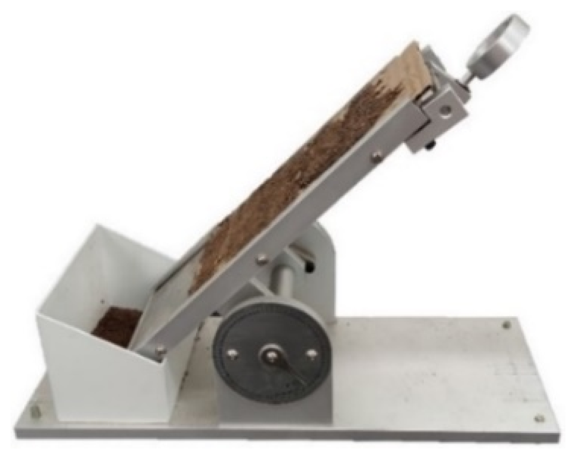
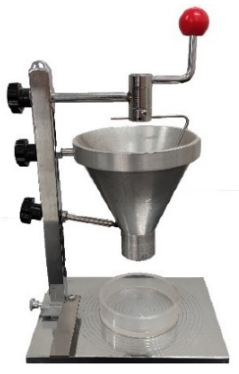
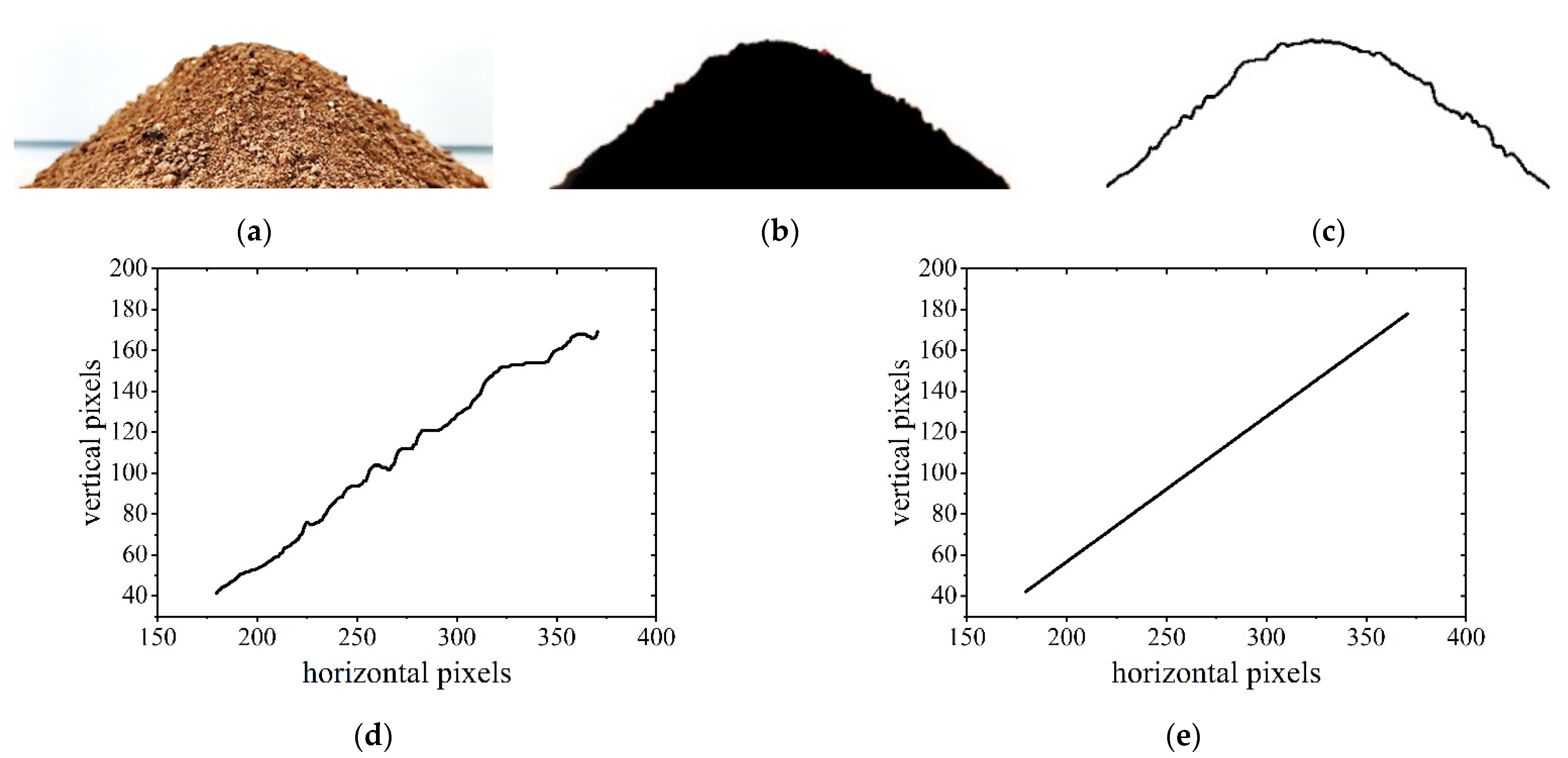
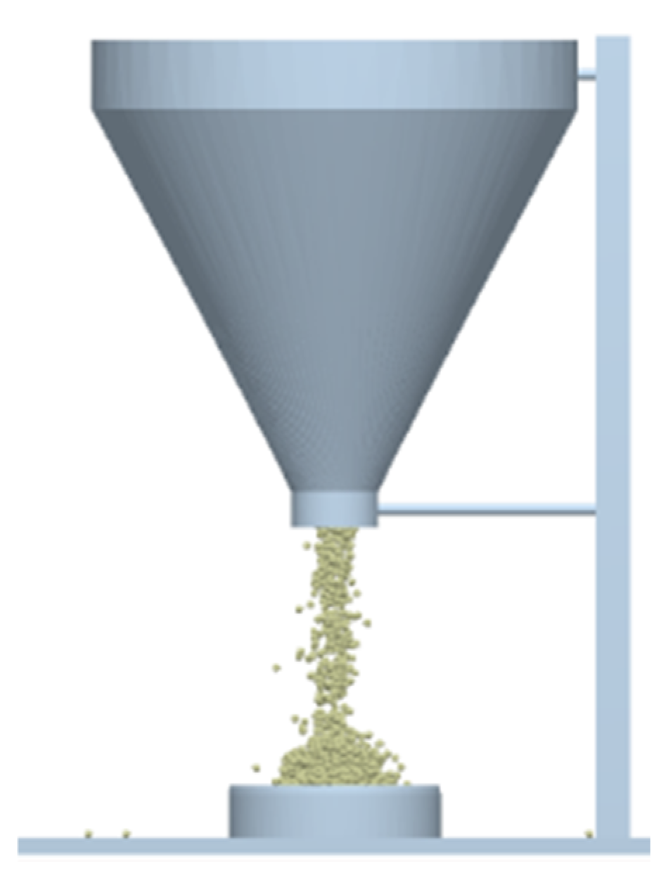
2.3.1. Determination of Angle of Repose in Soil with Different Moisture Content

We took 200 g of finely ground sandy soil powder after sieving and added 6, 12, 18, and 24 g of water to obtain soil with 3, 6, 9, and 12% water content, respectively. The rest angle meter was placed horizontally and the position of the soil extraction ring knife was adjusted to ensure that its center axis coincided with the funnel axis. Then, we poured the configured soil into the funnel from the inlet, waited for all of it to flow out from the outlet, and then waited for 120 s [13,20]. We then took pictures of the resting angle at the observation position, with the camera lens facing the stacked material. It was verified that when the lens deviation distance was ±5 cm and the deviation angle was ±5°, the resting angle error was kept at about 0.5%, which had less influence on the test results, so the shooting process should keep the lens position and angle within that range.

We imported the photos into D × O ViewPoint, corrected the shooting position and angle, imported them into Photoshop, cropped them, and obtained 804 horizontal pixels, as shown in Figure 3a. Then, we adjusted the color scale, removed the noise, and obtained a very high-contrast photo, as shown in Figure 3b.

The corrected photos were imported into MATLAB to be processed sequentially by grayscale and binarization, and an algorithm was used to determine the stacking angle boundary line, half of which was taken to draw a scatter plot, as shown in Figure 3c,d. The noise was processed and a linear fit was performed for the boundary value to obtain the coefficients of the fitted linear function, and the fitted image is shown in Figure 3e. The measured rest angle (α₁) was calculated from the value of k, and the calculation method is shown in Equation (1).

$${\alpha }_1=\arctan k$$

(1)

2.3.2. Determination of Rolling Friction Angle of Soil with Different Moisture Content

The soil–soil static friction coefficient and rolling friction coefficient range were determined by using a CNY-1 slope meter. We took rigid cardboard, applied glue on one side, and pasted soil with different moisture content evenly on it so that the surface was as flat as possible and without gaps. Since water is volatile, the next test should be conducted in a timely manner after preparation. The inclinometer was adjusted so that its pointer was at zero, the cardboard was fixed on the inclinometer, and a small amount of soil with the same moisture content was spread in an even layer on the right edge of the inclinometer. Then, the inclinometer was slowly rotated counterclockwise until the soil particles started to move, and the decline was accelerated. The inclinometer was stopped and the scale value (θ₁) was recorded. The inclinometer was adjusted to θ₁–15° moving [23], and we observed whether the soil continued to move to the leftmost side. If not, we continued to reduce the angle by 0.5° and repeated the test until it moved to the leftmost side of the inclinometer at a uniform speed and recorded the scale value (θ₂). Based on the analysis of the force, the angle of the inclinometer, and the coefficients of static friction (μ₁) and rolling friction (μ₂) the conversion relationships are shown in Equations (2) and (3):

$${\mu }_1=\tan {\theta }_1$$

(2)

$${\mu }_2=\tan {\theta }_2$$

(3)

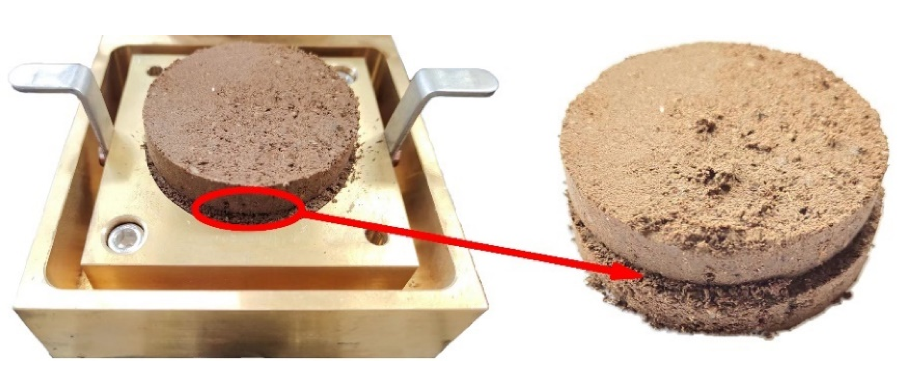
2.3.3. Direct Shear Test for Soil with Different Moisture Content and Firmness

In order to obtain the tangential stiffness per unit area and critical tangential stress of bond parameters in EDEM, a direct shear test was conducted on soil samples with different moisture content and firmness to determine their ability to resist transverse shear. The direct shear test was performed using a strain-controlled direct shear instrument, which involved applying pressure P to the shaft end of the cylindrical soil block, fixing the lower shear box, and pulling the upper shear box while slowly increasing shear force T. A soil sample taken after the direct shear was completed is shown in Figure 4. At this point, the axial stress σ is

$$\sigma =\frac{P}{A}$$

(4)

and tangential stress τ (at ultimate damage state) is

$$\tau =C_{0}R$$

(5)

where A is the soil cross-sectional area (diameter D = 61.8 mm, A = 3000 mm²), C₀ is the calibration coefficient of the force measuring ring, and R is the maximum reading of the micrometer in the force measuring ring.

Different axial stress σ can obtain different tangential stress τ, which is tested by increasing the weight to change the axial pressure. The test was completed to plot the curve of tangential stress σ under different axial stress τ conditions, fitting the straight line to obtain the expression of the primary linear function (i.e., Cullen formula):

$$\tau =\sigma \tan \phi +c$$

(6)

where φ is the angle of internal friction and c is the internal cohesion.

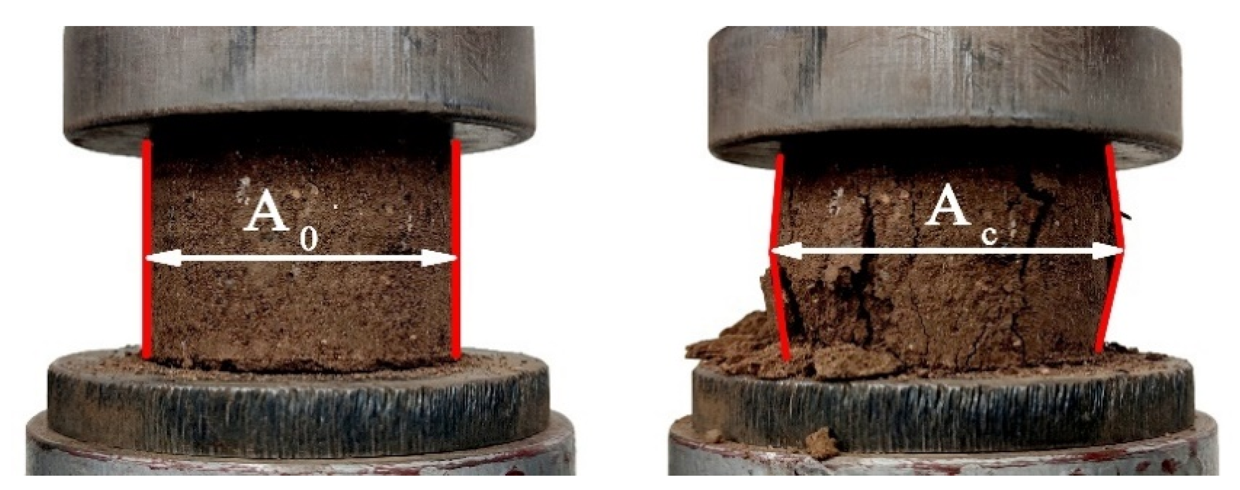
2.3.4. Lateral Limitless Compressive Test for Soil with Different Moisture Content and Firmness

The ability of soil to resist normal compression deformation also represents one of its important parameters. In order to obtain the normal stiffness per unit area and critical normal stress of the bond parameter in EDEM, the normal parameters of soil with different moisture content and firmness can be measured by using the no-lateral-limit compression test. The test uses a universal testing machine to slowly compress the prepared cylindrical soil samples at a uniform speed without a lateral limit to measure the pressure and stress magnitude in the ultimate damage state.

During the test, the peak of the axial load during uniform compression is recorded, as well as the radius of correction of the section at the peak point, from which the unconfined compressive strength of the soil is calculated. In the uniform compression process, the cylindrical soil sample will continue to deform under the real-time feedback compression pressure of the universal testing machine, until the pressure curve reaches a peak, and the peak pressure is recorded. If the curve shows a continuous upward trend and no peak curve appears, the pressure magnitude corresponding to the axial strain is recorded when it reaches 15% [24]. A soil specimen before and after compression is shown in Figure 5. The damaged cross-sectional area changed significantly compared with the initial cross-sectional area, which should be corrected; the corrected cross-sectional area A_c is

$$A_c=\frac{A_0}{1-\epsilon }$$

(7)

where A₀ is initial cross-sectional area of the soil block (mm) and ε is total strain when the soil mass is damaged.

The unconfined compressive strength of the soil can be obtained from the peak pressure or the pressure corresponding to an axial strain of 15% σ_u:

$${\sigma }_u=\frac{10F_{\max }\left(1-\epsilon \right)}{A_0}$$

(8)

where F_max is peak pressure or the corresponding pressure when the axial strain reaches 15%, that is, the load at the time of destruction (kN).

For the test, the specimen height was set to 40 mm with a cross-sectional diameter of 61.8 mm, and the universal testing machine was run at a constant speed of 1 mm/s to push the bottom disc under the loading compression [25] until it reached the peak of the time–pressure curve or axial strain of 15%, that is, at an axial loading length of 12 mm, the universal testing machine was stopped and the data pressure size and the section correction area were recorded after the return.

2.4. Experimental Results

2.4.1. Rest Angle and Friction Coefficient of Soil with Different Water Content

To measure the angle of repose and friction angle, each group of tests was repeated 10 times and the average values were taken as the final results after excluding outliers. The coefficient of rolling friction and coefficient of static sliding friction, and the calculated rest angle by coefficients of the linear function of the fitted rest angle image boundary with different moisture content soil are shown in

Table 1. Friction coefficient and rest angle of soil with different water content.

Water Content	Static Friction Coefficient (μ1)		Rolling Friction Coefficient (μ2)		Resting Angle(°)
	Min	Max	Min	Max
3%	0.6400	0.7813	0.1663	0.2543	32.76
6%	0.7265	0.8098	0.1877	0.2095	35.53
9%	0.7813	0.8391	0.2543	0.3249	37.89
12%	0.9014	0.9325	0.3265	0.3839	43.87

.

2.4.2. Results of Direct Shear Tests of Soil with Different Moisture Content and Firmness

A single-factor test of direct shear was conducted on soil with different water content and firmness. When soil firmness was used as the variable, the water content was controlled at a level of 6% and soil firmness was divided into five levels at equal intervals from 0.34 to 2.76 MPa; when soil water content was used as the variable, soil hardness was controlled at 1.55 MPa and soil water content was divided into four levels from 3 to 12%. The direct shear speed was set to 0.013 mm/s (0.8 mm/min) [26], the maximum distance of direct shear was 5 mm, and it took 6~7 min to directly shear a group. The force loop value was read once every 0.8 mm of direct shear, and after the direct shear the peak value was taken for calculation and fitting to obtain the values of cohesion and internal friction angle, and the results are shown in

Table 2. Results of direct shear tests on soil with different moisture content and firmness.

Water Content (%)	Solidity (MPa)	Cross-Sectional Area (mm2)	Direct Shear Displacement (mm)	Cohesion C (α = 0) (MPa)	Internal Friction Angle φ (°)	Tangential Stiffness per Unit Area N (m·m2)
6	0.34	3000	5	0.0165	32.5	3.3000 × 106
	0.945			0.0282	38.4	5.6480 × 106
	1.55			0.0587	32.3	1.1734 × 107
	2.155			0.0563	40.3	1.1262 × 107
	2.76			0.0626	37.3	1.2514 × 107
3	1.55			0.0866	21.5	1.7314 × 107
9				0.0575	35.4	1.1490 × 107
12				0.0818	19.2	1.6360 × 107

.

2.4.3. Results of Lateral Limitless Compressive Test of Soil with Different Moisture Content and Firmness

Similar to the direct shear test, a single-factor test of unconfined lateral limit resistance was conducted at the same factor level. The compression speed of the universal testing machine was set to 0.1 mm/s, and the sensor pressure data were recorded at a frequency of 5 Hz to calculate the unconfined compressive strength. The test results are shown in

Table 3. Results of unconfined compressive tests on soil with different moisture content and firmness.

Water Content (%)	Solidity (MPa)	Load (N)	Section Correction Radius (mm)	Corrected Area (mm2)	Axial Displacement (mm)	Compressive Strength without Lateral Limit (MPa)	Normal Stiffness per Unit Area N (m·m2)
6	0.34	298.6	31.83	3182.9011	2.87	0.0943	3.2688 × 107
	0.945	856	33.56	3538.2929	1.99	0.2431	1.2157 × 108
	1.55	895.6	33.25	3473.2270	2.41	0.2591	1.0700 × 108
	2.155	916.2	31.21	3060.1126	2.96	0.3006	1.0115 × 108
	2.76	1060	33.75	3578.4704	2.32	0.2962	1.2773 × 108
3	1.55	34.4	28.92	2627.5225	1.14	0.0114	1.1484 × 107
9		994	33.79	3586.9577	1.02	0.2771	2.7168 × 108
12		1043	32.14	3245.2011	2.73	0.3205	1.1775 × 108

, indicating that soil samples with different moisture content and firmness had different physical properties of compressive resistance. With increased soil solidity and water content, the unconfined compressive strength tended to increase.

3. Soil Parameter Discrete Element Calibration

3.1. Purpose of the Experiment

In order to determine the accurate values of contact parameters of sandy soil with different water content in potato growing areas, the level interval of the simulation test was determined by combining the physical test data, and the established simulation model was subjected to a parameter search for optimization. In order to verify the reliability of the bonding parameters for soil with different water content and hardness, bonding key simulation modeling was performed using the measured parameters, and discrete element simulation was performed for the unconfined compressive test and direct shear test to compare the errors of the actual and simulated tests. The reliability of the parameters was found to be high.

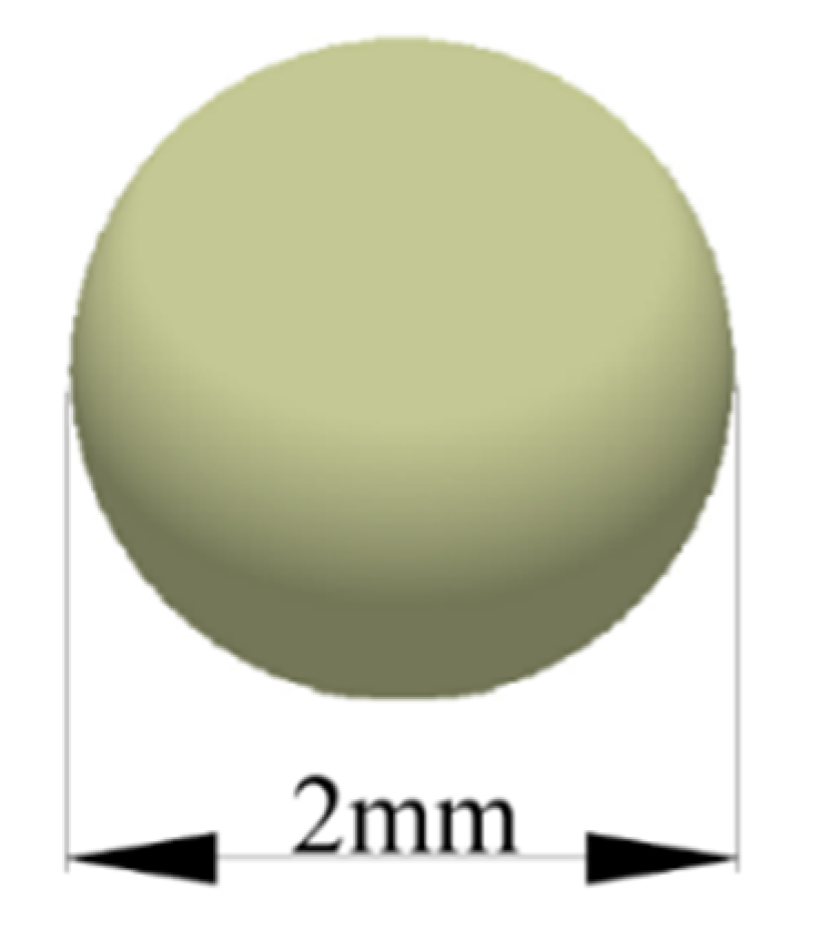
3.2. Soil Particle Simulation Parameters and Discrete Element Modeling

The soil–soil contact parameters include static friction, rolling friction, and recovery coefficients. It is known from the literature that the Poisson’s ratio of sandy soil physical parameters is 0.15–0.25 [27], taken as 0.2, and the modulus of elasticity is 7–20 MN/m² [19], taken as 13.5 MN/m². The parts of the rest angle tester that are in direct contact with the soil are made of steel with a density of 7865 kg/m³, Poisson’s ratio of 0.3, and shear modulus of 79,000 MPa.

Soil particle density, also known as soil specific gravity, depends on the type and relative content of solid-phase constituent substances. A forestry industry standard, Determination of soil particle density in forest soils [28], defines soil particle density as the ratio of the mass of the solid part of the soil (without water) to the mass of the same volume of water (40 °C). Therefore, soil particle density is not related to soil water content, soil porosity, etc. The density of sieved sandy soil particles was measured using the density bottle method, and the result was 1.38 g/cm³. Reviewing the relevant literature [22,27], some simulation parameters were obtained, as shown in

Table 4. Parameters of discrete element simulation.

Parameters	Materials
	Soil Particles	Steel
Poisson’s ratio	0.2	0.3
Shear modulus (MPa)		79,000
Modulus of elasticity (MPa)	13.5
Density (kg/m3)	1380	7865

.

According to the soil particle size distribution, the ratio of sand, powder, and mucilage is about 0.91:0.08:0.01, so the mucilage component was ignored in the modeling, the proportion of sand particles with 2 mm diameter was set to 90%, and the proportion of powder particles with 0.02 mm diameter was set to 10%. Since the particles were very small, the roundness of their shape was ignored, and they were set to a spherical shape uniformly and modeled as shown in Figure 6.

The 3D model of the rest angle meter was built by using SOLIDWORKS 2017 software, and the model size was kept consistent with the actual size and imported into the EDEM 2020 software. The contact model was set to choose the Hertz–Mindlin model with the JKR contact model and the particle generation mode was dynamic generation at 20,000 particles per second. The simulation process is shown in Figure 7.

3.3. Discrete Element Parameter Calibration and Result Analysis

3.3.1. Evaluation Indicators

The index of the test results is the ratio of the difference between the measured rest angle and the simulated rest angle to the measured rest angle, which was calculated as shown in Equation (9) after reviewing the literature:

$$y=\frac{\alpha -{\alpha }_1}{{\alpha }_1}\times 100\%$$

(9)

where α₁ is the measured rest angle and α is the discrete element simulation rest angle.

3.3.2. Plackett–Burman Test

The Plackett–Burman experimental design was used to analyze the significance of the simulation parameters with the rest angle as the response value and to screen the most significant factors. Through the preliminary experimental investigation, a total of seven discrete meta-parameters were determined for screening, which are denoted by x₁–x₇. The range of values was determined by referring to previous studies [19,20,24] and in combination with physical tests, as shown in

Table 5. Plackett–Burman test factor codes.

Parameter	Code	Low Level(−1)	High Level (+1)	Level Selection Source
Soil–65 Mn steel recovery factor	$x_1$	0.2	0.5	[19]
Soil–65 Mn steel static friction coefficient	$x_2$	0.5	1.2	[19]
Soil–65 Mn steel rolling friction coefficient	$x_3$	0.05	0.4	[19]
Soil–soil recovery factor	$x_4$	0.15	0.75	[20]
Soil–soil static friction coefficient	$x_5$	0.6	1.0	Friction coefficient determination
Soil–soil rolling friction coefficient	$x_6$	0.1	0.4	Friction coefficient determination
JKR water content model coefficient	$x_7$	0	0.75	[24]

. The Plackett–Burman test design and results are shown in

Table 6. Plackett–Burman experimental design and results.

No.	Factors							Rest Angle (°)
	X1	X2	X3	X4	X5	X6	X7
1	1	−1	1	−1	−1	−1	1	40.07
2	1	−1	1	1	−1	1	−1	18.63
3	0	0	0	0	0	0	0	32.47
4	−1	1	1	1	−1	1	1	46.20
5	−1	1	1	−1	1	−1	−1	14.00
6	0	0	0	0	0	0	0	36.37
7	1	1	1	−1	1	1	−1	32.96
8	−1	−1	−1	1	1	1	−1	25.97
9	−1	−1	1	1	1	−1	1	22.16
10	0	0	0	0	0	0	0	41.97
11	1	−1	−1	−1	1	1	1	64.70
12	1	1	−1	1	−1	−1	−1	4.69
13	−1	1	−1	−1	−1	1	1	72.16
14	1	1	−1	1	1	−1	1	21.72
15	−1	−1	−1	−1	−1	−1	−1	9.15

; a total of 15 sets of tests were required. To ensure the accuracy of the test and verify the test error, three sets of central level tests were added.

The PB test results were analyzed, and the results are shown in

Table 7. Analysis of Plackett–Burman test results.

Source	DF	Standardized Effect	MS	Impact Rate	p-Value	Significance
Models	8		613.49	96.66%	<0.001	***
X1	1	0.3722	3.91	0.08%	0.723
X2	1	0.6005	10.18	0.20%	0.57
X3	1	1.3233	49.44	0.97%	0.234
X4	1	5.0889	731.13	14.40%	0.007	**
X5	1	0.5114	7.38	0.15%	0.627
X6	1	8.0859	1845.89	36.36%	<0.001	***
X7	1	8.7801	2176.4	42.87%	<0.001	***
Bend	1		83.59	1.65%	0.136
Error	6		28.23	3.34%
Total	14			100.00%

** Statistically significant difference; *** Extremely statistically significant difference.

. The order of significant factors is: JKR water content model coefficient X₇ > soil–soil rolling friction coefficient X₆ > soil–soil recovery coefficient X₄, with influence rates of 42.87, 36.36, and 14.40%, respectively, and the rest of the factors are not significant.

Combined with the test principle, the analysis showed that in the process of rest angle determination, the soil only had contact with 65 Mn steel before the ring knife was spread; the rest of the time there was only collision and friction between soil and soil, and the rest angle after the soil overflow was more accurate, so the contact parameter between 65 Mn steel and soil was not the decisive parameter affecting the rest angle. After the soil particles were in contact with each other, their movement state changed from rolling to static; first, they were subjected to the effect of rolling friction, and there was relative movement between particles. The JKR surface energy essentially increased the viscosity of the surface of the soil particles and enhanced the bonding force between particles.

3.3.3. Steepest Climb Test

The significant factors were obtained from the results of the Plackett–Burman test, with reference to the values measured in the physical test and using the steepest climb test. The Box–Behnken test was used with the recovery coefficient between soil particles X₄, rolling friction coefficient X₆, and JKR water content model coefficient X₇ as the test factors and the rest angle simulation test error of soil particles as the response value. The angle of repose was calculated by MATLAB at the end of the test to obtain the simulated angle of repose, which was compared with that of actual soil with different water content to obtain the error rate. The test scheme and test results are shown in

Table 8. Steepest climbing test arrangement and results.

No	Factors			Resting Angle (°)	Error Rate (°)
	X4	X6	X7		3%	6%	9%	12%
1	0.15	0.10	0	15.22	0.5354	0.5716	0.5984	0.6530
2	0.25	0.15	0.125	31.72	0.0317	0.1072	0.1630	0.2769
3	0.35	0.20	0.250	41.76	0.2748	0.1754	0.1020	0.0480
4	0.45	0.25	0.375	39.96	0.2198	0.1247	0.0545	0.0890
5	0.55	0.30	0.500	42.61	0.3007	0.1993	0.1244	0.0286
6	0.65	0.35	0.625	45.26	0.3816	0.2739	0.1944	0.0318
7	0.75	0.40	0.750	68.95	1.1047	0.9407	0.8196	0.5718

, where it can be seen that the smallest error rate of the target parameters with different water content lies between numbers 2 and 6.

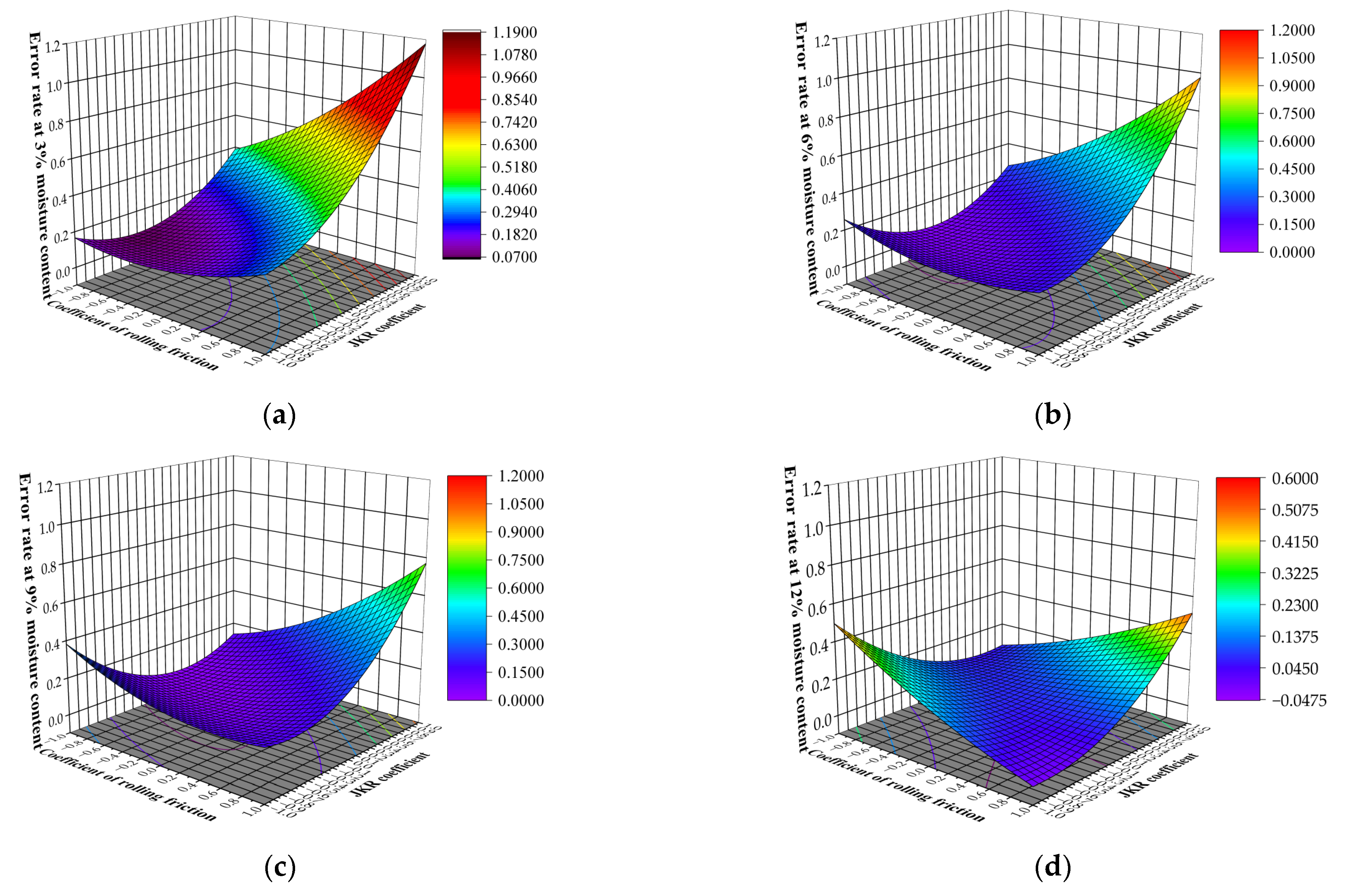
3.3.4. Box–Behnken Test Design and Analysis of Results

The range of Box–Behnken test factor values can be determined using the steepest climb test, with the level of each parameter of number 6 as high (+1), number 2 as low (−1), and number 4 as intermediate (0). Three center points were used in the test process to evaluate the error of the test results, and 15 trials were required. The test procedure and results are shown in

Table 9. Box–Behnken experimental design and results.

No.	Factors			Rest Angle (°)	Error Rate (°)
	X4	X6	X7		3%	6%	9%	12%
1	0(0.45)	−1 (0.15)	1 (0.625)	42.65	0.3017	0.2003	0.1255	0.0279
2	−1 (0.25)	1 (0.35)	0 (0.375)	51.36	0.5678	0.4456	0.3556	0.1708
3	0	1	1	68.57	1.0932	0.9300	0.8098	0.5631
4	0	0 (0.25)	0	39.01	0.1907	0.0979	0.0295	0.1108
5	0	−1	−1 (0.125)	24.28	0.2590	0.3168	0.3593	0.4467
6	0	1	−1	45.37	0.3849	0.2769	0.1974	0.0342
7	1 (0.65)	−1	0	33.50	0.0227	0.0570	0.1157	0.2363
8	1	1	0	47.39	0.4465	0.3337	0.2506	0.0802
9	−1	0	−1	32.50	0.0080	0.0854	0.1423	0.2592
10	1	0	−1	33.06	0.0093	0.0694	0.1274	0.2463
11	0	0	0	41.67	0.2720	0.1728	0.0997	0.0502
12	1	0	1	55.43	0.6919	0.5600	0.4628	0.2634
13	−1	0	1	59.33	0.8110	0.6698	0.5658	0.3523
14	−1	−1	0	34.53	0.0540	0.0282	0.0887	0.2129

.

For the Box–Behnken test, an ANOVA was conducted for four water content conditions, and the results are shown in

Table 10. Analysis of variance of Box–Behnken experimental regression model under different water content conditions.

Source	3% Moisture Content		6% Moisture Content		9% Moisture Content		12% Moisture Content
	p-Value	Significance	p-Value	Significance	p-Value	Significance	p-Value	Significance
Models	0.0092	**	0.006	**	0.0036	**	0.0065	**
X4	0.4593		0.4435		0.3511		0.3246
X6	0.0027	**	0.0027	**	0.0047	**	0.6462
X7	0.0012	**	0.0014	**	0.0019	**	0.2138
X4 × X6	0.7215		0.4642		0.3723		0.3452
X4 × X7	0.6353		0.62		0.5421		0.5182
X6 × X7	0.0385	**	0.0075	**	0.0015	**	0.0003	***
X42	0.4837		0.9241		0.2809		0.1086
X62	0.2402		0.1431		0.0489	**	0.1895
X72	0.0281	**	0.0061	**	0.0018	**	0.0034	**
Lack of Fit	0.0728	Not significant	0.1107	Not significant	0.1672	Not significant	0.1882	Not significant
R2	0.9499		0.9583		0.9661		0.9568
Adeq Precision	11.8888		13.2918		14.0464		11.8414

** Statistically significant difference; *** Extremely statistically significant difference.

. It can be seen that the p-values of the four water content models were p_3% = 0.0092, p_6% = 0.006, p_9% = 0.0036, and p_12% = 0.0065, all less than 0.01, indicating high significance, and the fitted R² was R²_3% = 0.9499, R²_6% = 0.9583, R²_9% = 0.9661, and R²_12% = 0.9568. The model correlation was very high, the signal-to-noise ratio measured by Adeq Precision was greater than 4, the model was less disturbed by external factors, the misfit term was not significant (lack of fit > 0.05), and the model credibility was high.

For soil with 3 and 6% water content, the rolling friction coefficient X₆ and JKR coefficient X₇ were significant and the recovery coefficient X₄ became insignificant, mainly due to the change in the Plackett–Burman and Box–Behnken test values, where the recovery coefficient was not a decisive parameter in changing the test results within the interval discussed for the Box–Behnken test. Examining the interaction between factors revealed that the rolling friction and JKR coefficient interaction X₆ × X₇ and JKR coefficient squared X₇² were significant; for soil with 9% water content, in addition to X₆, X₇, X₆ × X₇, and X₇², the rolling friction coefficient squared X₆² was significant; for soil with 12% water content only X₆ × X₇ and X₇² were significant. Response surface analysis plots were made for X₆ and X₇, as shown in Figure 8a–d.

Excluding the insignificant factors, the quadratic polynomial equation between significant factors and rest angle error rate under different water content conditions was obtained as:

$$Y_{3\%}=0.237+0.2319X_6+0.2796X_7+0.1664X_6{X}_7+0.19X_7{}^2$$

(10)

$$Y_{6\%}=0.1405+0.173X_6+0.201X_7+0.1924X_6{X}_7+0.2102X_7{}^2$$

(11)

$$Y_{9\%}=0.0695+0.1155X_6+0.1422X_7+0.2116X_6{X}_7+0.0908X_6{}^2+0.2127X_7{}^2$$

(12)

$$Y_{12\%}=0.0763+0.2369X_6{X}_7+0.1485X_7{}^2$$

(13)

Combining Equations (10)–(13), the limiting equation that can be solved was obtained as Equation (14):

$$\{\begin{array}{l}\min Y_{3\%},Y_{6\%},Y_{9\%},Y_{12\%}\\ s.t.\{\begin{array}{l}{X}_4=0.45\\ -1\le X_6\le 1\\ -1\le X_7\le 1\end{array}\end{array}$$

(14)

Combined with physical tests, the polynomial was solved using Design-Expert software, and since the recovery coefficient X₄ was not significant under various water content conditions, an intermediate value of 0.45 was used, and the optimal solution was obtained by analyzing the soil rolling friction coefficient X₆ and JKR coefficient X₇. The result showed X₆ = 0.188 and X₇ = 0.3558 for 3% water content soil; X₆ = 0.15 and X₇ = 0.356 for 6% water content soil; X₆ = 0.193 and X₇ = 0.363 for 9% water content soil; and X₆ = 0.338 and X₇ = 0.371 for 12% water content soil (

Table 11. Contact parameters for soil with different water content.

Parameter	3% Moisture Content	6% Moisture Content	9% Moisture Content	12% Moisture Content
Soil–soil recovery coefficient	0.45	0.45	0.45	0.45
Soil–soil rolling friction coefficient	0.188	0.15	0.193	0.388
JKR surface energy coefficient	0.3558	0.3560	0.3630	0.371

).

3.4. Discrete Element Contact Parameter Calibration Validation

Parametric validation of the test results was performed to obtain the rest angle models for soil with water content of 3, 6, 9, and 12%, as shown in Figure 9. The fit coefficient of soil was calculated to be 0.649, 0.707, 0.771, and 0.894, and the rest angle was 32.98°, 35.26°, 37.63°, and 41.80°, respectively, compared to actual measured values, the maximum error rate was 4.72%, which was kept within 5%, and the errors were within acceptable limits, indicating that the calibration parameters were reliable and consistent with the actual soil mechanical contact parameters.

3.5. Soil Direct Shear Test Discrete Element Simulation

EDEM 2020 software was used to simulate the soil direct shear process. The generated soil particles were compacted before the direct shear to reduce their spacing, and bonds were generated afterwards. A permeable stone was placed on the surface of the direct sheared soil and the soil was compacted with a force of 12 N. The model was set as Hertz–Mindlin with JKR as well as bonding, the parameters were set as the actual parameters of calibration, and several tests were conducted to measure the peak shear force under the base 0.1 MPa positive pressure condition. The relative error was compared with the cohesive force C of the direct shear test, and the overall stage of simulated bonding key force is shown in Figure 10. Figure 10a shows the initial state before the start of direct shear, with overall force distribution of bonding inside the soil and no special force points, in line with the bonding characteristics of the soil before direct shear. Figure 10b shows the state of bonding of the soil just before the start of direct shear. It can be seen from the figure that the shear surface force is larger, the maximum force point is located on the front and rear of the direct shear direction, and at this time the soil is still in the bonding state and has not yet ruptured. Figure 10c shows the maximum stress period in the process of direct shear. Although the soil is in the bonding state and has reached the limit of damage, the maximum stress is located on the shear surface and expands outward. Trace displacement appears on the front and rear end of the direct shear direction of the shear surface soil due to the presence of bonding forces, and the rest of the region of soil stress is not changed. Figure 10d shows the state after the end of direct shear; at this time, the shear force no longer exists, most bonds have been broken, only a small amount remains in the limit fracture state, the total stress is reduced, and the soil has been damaged by shear.

After the direct shear was completed, the force of the lower shear box was observed to find the peak force point, as shown in

Table 12. Comparison of peak shear force under 0.1 MPa positive pressure in the direct shear test.

Water Content (%)	Solidity (MPa)	Cross-Sectional Area (mm2)	Direct Shear Displacement (mm)	Peak Shear Force (N)		Error Rate (%)
				Physical Tests	Simulation Test
6	0.34	3000	5	149.4	143.9	3.68
	0.945			183.1	176.3	3.71
	1.55			197.4	184.5	6.53
	2.155			209.2	198.9	4.92
	2.76			262.9	246.5	6.24
3	1.55			157.3	162.3	3.18
9				204.9	192.8	5.91
12				165.3	174.7	5.69

. Comparing the peak force of the soil shear process under the 0.2 MPa positive pressure condition of the physical test, the error rate was found to be distributed in the range of 3.71–6.53%, which was within the tolerable range, and the overall change trend was consistent, indicating that the soil sample parameters of the physical and simulation tests of direct shear were basically consistent, and the measured values are real and reliable.

3.6. Discrete Element Simulation of the Soil Lateral Limitless Compressive Test

The EDEM simulation software was used to simulate the unconfined compressive test of the soil by first compacting the soil to form a compressed soil block with a cross-sectional area of 3000 mm² and a height of 40 mm, generating a bonding key, and compressing it at a rate of 0.1 mm/s. The model was set to Hertz–Mindlin with JKR and bonding. The parameters were set to the actual calibrated parameters, and multiple tests were conducted to observe the peak value of the time–pressure curve or, if there was no peak, the corresponding pressure value when the axial strain reached 15%, and the physical tests were compared to verify the error. Figure 11a–d shows the force distribution of bonding during the unconfined compressive test.

Figure 11a shows the force distribution state of the soil bond at the beginning of compression, when all the soil compression stress is concentrated on the lower surface of the soil and gradually expands upward, and the soil remains bonded. Figure 11b,c shows the front and top views when the soil was subjected to maximum stress. The stress was mainly concentrated on the upper and lower surfaces of the soil and connected in an hourglass shape, and the middle section of the soil was slightly convex, which shows that the center was compressed outward. It can be seen from the top view that the central part of the lumpy soil was subjected to the greatest stress, which extended outward from the center, and the outer ring was relatively less stressed. Figure 11d shows the stress state of the soil at the end of compression; at this time, due to the higher degree of compression, a larger number of bonds were broken and the total stress was reduced, indicating that the soil pattern was destroyed. After the compression was completed, the EDEM software was used to construct the time–stress graph of the compressed plate, and the peak value of the discounted graph was observed, as shown in

Table 13. Comparison of physical and simulation tests of unconfined compression.

Water Content (%)	Solidity (MPa)	Peak Axial Force or 15% Axial Strain Corresponding Pressure(N)		Error Rate (%)
		Physical Test	Simulation Test
6	0.34	94.253634	101.83	8.04
	0.945	243.05506	226.13	6.96
	1.55	259.12501	273.9	5.70
	2.155	300.64253	289.11	3.84
	2.76	296.21595	311.23	5.07
3	1.55	11.417599	10.59	7.25
9		277.11506	299.47	8.07
12		320.4732	318.555	0.60

. This shows that the parameters of the bonding key in the simulation test were basically the same as those measured in the physical test, and the reliability of the test was high.

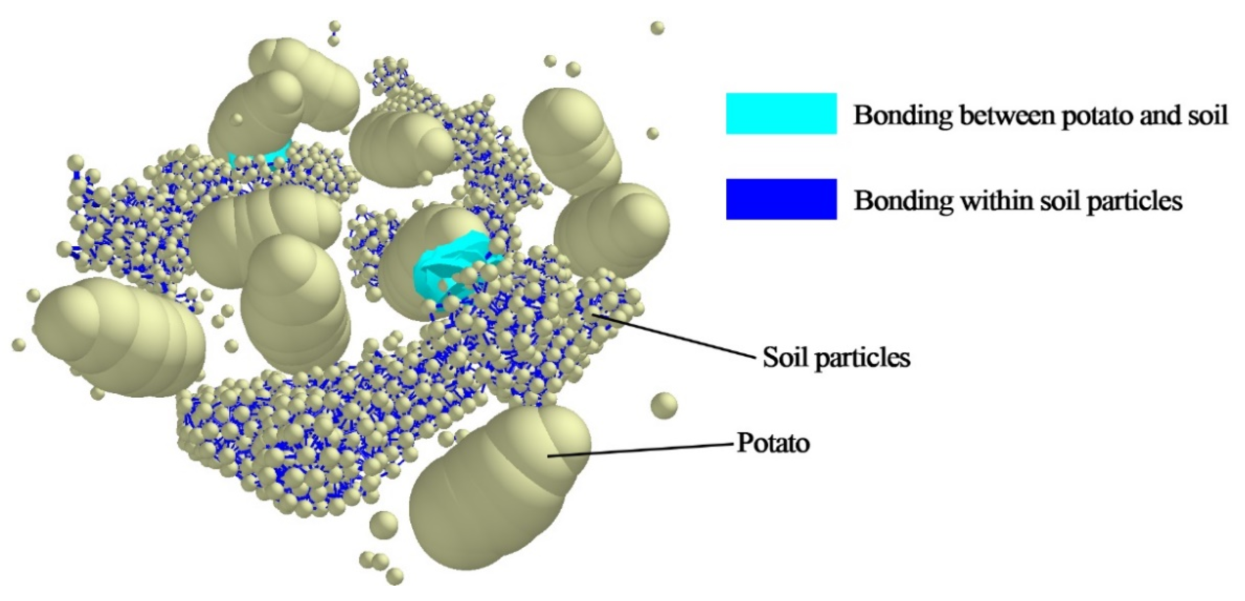
3.7. Discrete Meta-Simulation of Potato–Soil Mixtures

Ultimately, we obtained the contact and bonding parameters of the soil, which provided a parametric basis for the discrete element simulation of potato–soil separation. In order to speed up the calculation speed of the simulation and improve the computational efficiency, we used the multi-sphere approach to simulate the potato shape and increased the radius of the circular particles to simulate the soil particles and observe their bond-bonding state. A simulation of the potato–soil mixture with bonded bonds is shown in Figure 12. The light blue area shows the bonding action between the potato and the soil, while the dark blue area shows the bonding action within the soil particles. As can be seen from the diagram, the soil is subjected to collision impact, the bonding bonds break, and some of the soil particles start to become dispersed. The simulation process of potato–soil separation provides a basis for improving the potato–soil separation device of the harvester and is of great practical importance.

4. Discussion

Understanding the fragmentation characteristics of soil agglomerates is crucial for optimizing and improving potato–soil separation devices for potato harvesters, but currently, many researchers have only explored potato damage, ignoring the physical properties of the soil.

We propose an approach for performing single-test simulation with multiple response surface analysis to calibrate contact parameters for soil with different water content, while establishing a DEM to simulate the aggregation state of soil through bonding aggregation of small spheroid particles. The method acquires the discrete element contact parameters and bonding parameters and reproduces the properties of soil shear and compressive strength using DEM software. The research in this paper was focused on (1) calibrating the contact parameters of soil with different moisture content, and (2) establishing soil agglomerate models to obtain shear and compressive strength parameters of soil using direct shear tests and unconfined lateral compressive tests.

4.1. Calibration of Soil Contact Parameters

The Hertz–Mindlin and JKR contact models have been commonly utilized as soil contact models in the literature when performing DEM simulations [29]. The Hertz–Mindlin contact model is suitable for non-cohesive materials, while the JKR contact model is more suitable for adhesive materials. The soil with water content that we calibrated is a typical cohesive material. In the combined Hertz–Mindlin and JKR contact model, the tangential contact force, normal damping force, and tangential damping force can be calculated similarly to the Hertz–Mindlin model. The normal contact force employs JKR theory to account for cohesion [30]. Therefore, in this paper, the Hertz–Mindlin with JKR contact model was used to simulate soil.

The contact parameters used in the simulation are the material-to-material friction coefficient, the recovery coefficient, and the JKR surface energy coefficient. In order to obtain these contact parameters for bulk sandy soil with different water content, we conducted a calibration test with the rest angle error as an indicator. We screened the three most significant factors from the seven factors as soil–soil recovery coefficient, soil–soil rolling friction coefficient, and JKR surface energy coefficient using the Plackett–Burman test, which is similar to the results obtained in numerous studies. For example, in [31], it was found that the static friction coefficient, rolling friction coefficient, and surface energy were the key parameters for wet bulk coal. Similarly, Li et al. [32] found that the most significant parameters for wheat flour were surface energy and rolling friction coefficient. Roessler et al. [33] presented a calibration method and found that the dominant parameters of wet sand were rolling friction and surface energy. Finally, Zhang et al. [34] calibrated the DEM parameters of rice and found that AoR was strongly influenced by rolling friction and restitution. It is noteworthy that they all used tiny spherical particles instead of irregularly shaped particles for the parameter calibration, so that rolling friction was a highly significant factor in all cases. In contrast, Zhu [15] et al. used the EDEM multi-sphere approach, which treats soil particles as miniature irregularly shaped particles for simulation, and the rolling friction is less significant compared to soil–soil static friction.

After the factors with significant effects were found, they were subjected to Box–Behnken response surface analysis. The Box–Behnken design (BBD) is an effective technique for parameter calibration [34,35]. It suggests how to select points from the three-level factorial arrangement, which allows efficient estimation of the first- and second-order coefficients of the mathematical model [36,37]. The BBD consists of a central point and several middle points located at the edges of a cube superimposed on a sphere [38]. The design is more efficient and economical because it greatly reduces the number of experiments. The experimental results revealed that the soil–soil recovery factor, which was significant in the Plackett–Burman test, became insignificant in the Box–Behnken test. The analysis revealed that the reason for this was the change in the horizontal range, for which a smaller interval was chosen in the Box–Behnken test, resulting in a smaller interval in the range of inquiry for the soil–soil recovery factor to have little influence on the test results. We conducted one Box–Behnken test, but the error rate of the rest angle for different water content conditions could be obtained. Using the error rate as an index for the test analysis and response surface analysis, the parameters of sandy soil with different water content conditions could be directly obtained. This method simplifies the experimental process, and the parameters can be solved directly for soil with certain water content collected in the future without the need for re-simulation.

4.2. Calibration of Soil Bonding Parameters

For slabby soil agglomerates, which we usually consider as relatively less hard rocks, we used the bonded-particle model (BPM) proposed by Potyondy and Cundall [39], which is widely used to model ore particles [40]. The key to BPM lies in the calibration of bonding parameters. The uniaxial compression test is commonly used for parametric calibration of the BPM [41]. For example, Manso et al. [42] established a particle model of Lac du Bonnet granite using 5400–15,000 sub spheres, and studied its mechanical properties using the uniaxial compression test. Jiang [43] built a model of ore particles using 3023 sub spheres with a radius of 0.5 mm and studied the mechanical properties through a uniaxial compression test. Johansson et al. [44] used 16,540–25,914 sub spheres with a radius of 1 mm to form ore particle models. They considered rock particles as agglomerates formed by the aggregation of small particles connected by bonding and explored the mechanical properties in shear or compression. Chen and Wang et al. [45] explored the effects of normal stiffness per unit area, shear stiffness per unit area, critical normal stress, critical shear stress, and the radius of filled spheres on the performance of bonded particle models using uniaxial compression tests. These parameters are necessary for DEM simulations, and we added a direct shear test to obtain these bonding parameters. The reliability of the parameters was then verified by discrete element simulation to prove the authenticity of the test.

5. Conclusions

• Based on EDEM 2020 software, the recovery coefficient, static friction coefficient, rolling friction coefficient, and JKR surface energy factor between soil particles and between soil and 65 Mn steel were selected as the test factors at 3, 6, 9, and 12%, the rest angle error rate of the physical and simulation tests was used as the evaluation index, and the Plackett–Burman test was used to screen the significant factors: JKR surface energy, interparticle recovery coefficient, and interparticle rolling friction factor of soil.
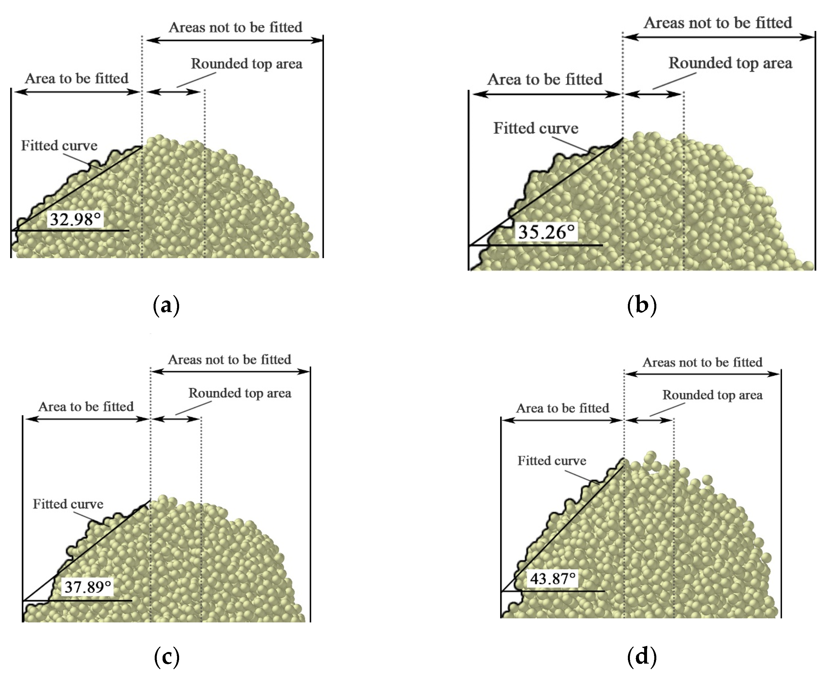
• A single simulation of multiple Box–Behnken response surface analysis was performed to optimize the model. The JKR surface energy coefficients were obtained as 0.3558, 0.356, 0.363, and 0.371 for soil with moisture contents of 3, 6, 9, and 12%, respectively, and the interparticle rolling friction was 0.188, 0.15, 0.193, and 0.338, respectively. The simulation was carried out using the above parameters, and the simulation rest angle was obtained as 32.98°, 35.26°, 37.63°, and 41.80°, respectively, with a maximum error rate of 4.72%.
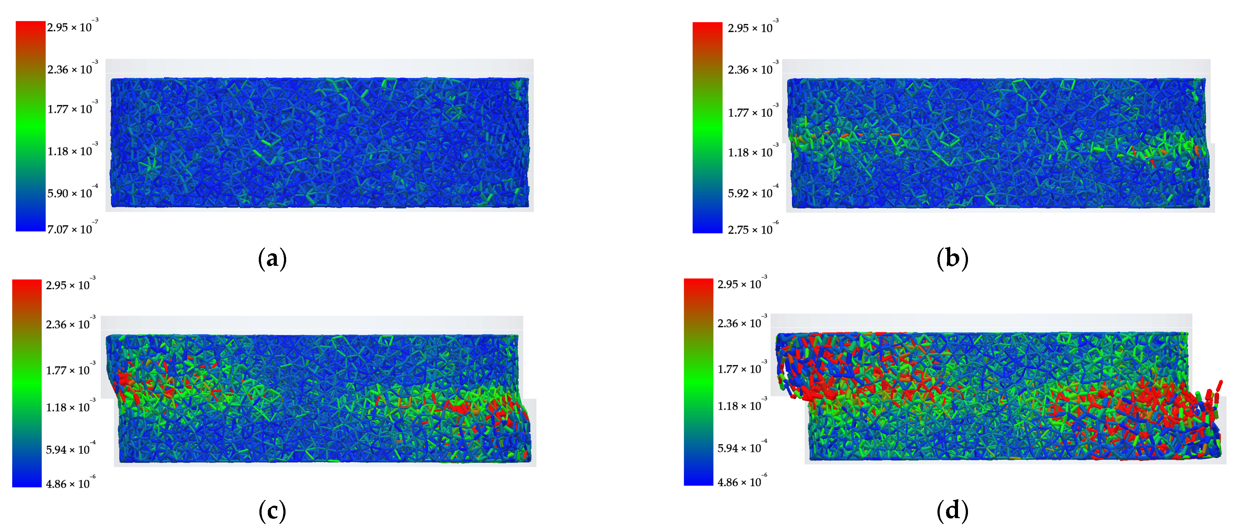
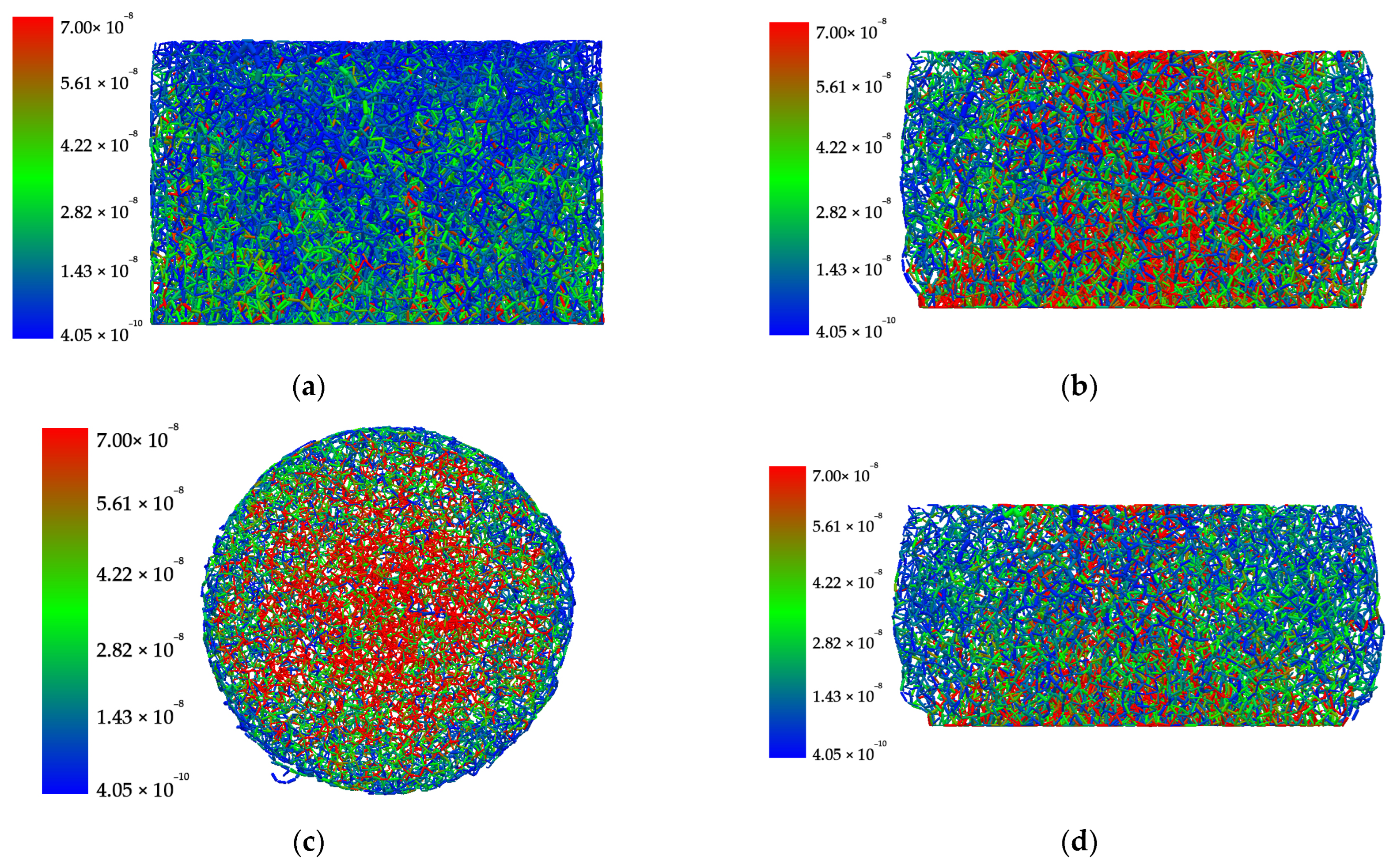
• The parameters required for the bonding key of the EDEM simulation were obtained using direct shear and lateral limitless compression tests. The EDEM simulation approach combining direct shear and unconfined compression tests was proposed to obtain the force distribution images of bonds in the shear and compression processes. The error rates of the simulation and physical tests for the direct shear test were distributed in the range of 3.71–6.53%, and those of simulation and physical tests for the unconfined compression test were distributed in the range of 0.6–8.07%, which were within tolerable limits, and the overall trend was consistent.

In this study, a model of sandy soil with different water content in potato growing areas was established, which provides reliable parameters for EDEM simulation of the process of separating potatoes from soil and has a catalyzing effect on the optimization of the potato harvester swing separation mechanism. At the same time, a parameter calibration method is proposed for slab soil with different water content, which has different textures in different areas. The method can calibrate the contact parameters of soil with different water content using a single test, which greatly reduces the workload and provides a new research idea for soil calibration.

References

1. Wei, Z.; Li, H.; Su, G. Development of potato harvester with buffer type potato-impurity separation sieve. Trans. Chin. Soc. Agric. Eng. 2019, 35, 1–11. [Google Scholar]
2. Ding, W.; Zhu, J.; Chen, W. Simulation calibration of highland barley contact parameters based on EDEM. J. Chin. Agric. Mech. 2021, 42, 114–121. [Google Scholar] [CrossRef]
3. Li, X.; Du, Y.; Liu, L.; Zhang, Y.; Guo, D. Parameter calibration of corncob based on DEM. Adv. Powder Technol. 2022, 33, 103699. [Google Scholar] [CrossRef]
4. Coetzee, C.J.; Els, D.N.J.; Dymond, G.F. Discrete element parameter calibration and the modelling of dragline bucket filling. J. Terramechanics 2009, 47, 33–44. [Google Scholar] [CrossRef]
5. Wu, Z.; Wang, X.; Liu, D.; Xie, F.; Ashwehmbom, L.G.; Tang, Z.Z. Calibration of discrete element parameters and experimental verification for modelling subsurface soils. Biosyst. Eng. 2021, 212, 215–227. [Google Scholar] [CrossRef]
6. Wen, X.; Fang, F.; Liu, Y. Research on stacking angle of coal particles and parameter calibration on EDEM. China Saf. Sci. J. 2020, 30, 114–119. [Google Scholar] [CrossRef]
7. Wang, L.; Fan, S.; Chen, H. Calibration of contact parameters for pig manure based on EDEM. Trans. Chin. Soc. Agric. Eng. 2020, 36, 95–102. [Google Scholar]
8. Rui, Z.; Dianlei, H.; Qiaoli, J.; Yuan, H.; Jianqiao, L. Calibration methods of sandy soil parameters in simulation of discrete element method. Nongye Jixie Xuebao/Trans. Chin. Soc. Agric. Mach. 2017, 48, 49–56. [Google Scholar] [CrossRef]
9. Fang, H. Research on the straw-soil-rotary blade interaction using discrete element method. Master’s Thesis, Nanjing Agriculture University, Nanjing, China, 2016. [Google Scholar]
10. Ding, Q.; Ren, J.; Adam, B.E.; Zhao, J.; Ge, S.; Li, Y. DEM analysis of subsoiling process in wet clayey paddy soil. Nongye Jixie Xuebao/Trans. Chin. Soc. Agric. Mach. 2017, 48, 38–48. [Google Scholar] [CrossRef]
11. Ajmal, M.; Roessler, T.; Richter, C.; Katterfeld, A. Calibration of cohesive DEM parameters under rapid flow conditions and low consolidation stresses. Powder Technol. 2020, 374, 22–32. [Google Scholar] [CrossRef]
12. Yu, W.; Liu, R.; Yang, W. Parameter Calibration of Pig Manure with Discrete Element Method Based on JKR Contact Model. AgriEngineering 2020, 2, 367–377. [Google Scholar] [CrossRef]
13. Xing, J.; Zhang, R.; Wu, P. Parameter calibration of discrete element simulation model for latosol particles in hot areas of Hainan Province. Trans. Chin. Soc. Agric. Eng. 2020, 36, 158–166. [Google Scholar]
14. Liu, Y.; Zhao, J.; Qi, H. Parameters calibration of discrete element of clay soil in yam planting area. J. Hebei Agric. Univ. 2021, 44, 99–105. [Google Scholar] [CrossRef]
15. Zhu, J.; Zou, M.; Liu, Y.; Gao, K.; Su, B.; Qi, Y. Measurement and calibration of DEM parameters of lunar soil simulant. Acta Astronaut. 2022, 191, 169–177. [Google Scholar] [CrossRef]
16. Jba, A.; Ma, A.; Ying, C.B.; Zz, B. Calibration of discrete element parameters of crop residues and their interfaces with soil. Comput. Electron. Agric. 2021, 188, 106349. [Google Scholar]
17. Aikins, K.A.; Ucgul, M.; Barr, J.B.; Jensen, T.A.; Antille, D.L.; Desbiolles, J.M. Determination of discrete element model parameters for a cohesive soil and validation through narrow point opener performance analysis. Soil Tillage Res. 2021, 213, 105123. [Google Scholar] [CrossRef]
18. Wei, Z.; Su, G.; Li, X. Parameter Optimization and Test of Potato Harvester Wavy Sieve Based on EDEM. Ransactions Chin. Soc. Agric. Mach. 2020, 51, 109–122. [Google Scholar]
19. Song, Z.; Li, H.; Yan, Y. Calibration Method of Contact Characteristic Parameters of Soil inMulberry Field Based on Unequal-diameter Particles DEM Theory. Trans. Chin. Soc. Agric. Mach. 2022, 53, 21–33. [Google Scholar]
20. Wang, Y. Soil Wind Erosion Characteristics and Wind Erosion Estimation in Dry Farming Areas of Wuchuan County. Master’s Thesis, Inner Mongolia Agriculture University, Hohhot, China, 2019. [Google Scholar]
21. Chinese Academy of Inspection and Quarantine; China Chemical Economic and Technological Development Center. Chemicals-Test method for particlesize analysis of soils. In General Administration of Quality Supervision, Inspection and Quarantine of the People’s Republic of China; Standardization Administration of the People’s Republic of China: Beijing, China, 2011; Volume GB/T 27845-2011, p. 20. [Google Scholar]
22. China Renewable Energy Engineering Institute; Nanjing Hydraulic R lesearch Institute. Standard for geotechnical testing method. In Ministry of Housing and Urban-Rural Development of the People’s Republic of China; State Administration for Market Regulation: Beijing, China, 2019; Volume GB/T 50123-2019, p. 717. [Google Scholar]
23. Xiao, Z.; Tian, H.; Zhang, T. Parameter calibration of discrete element numerical simulation for the dedusting sieve of corn straw feed. J. China Agric. Univ. 2022, 27, 172–183. [Google Scholar]
24. Xie, F.; Wu, Z.; Wang, X. Calibration of discrete element parameters of soils based on unconfined compressive strength test. Trans. Chin. Soc. Agric. Eng. 2020, 36, 39–47. [Google Scholar]
25. Li, G.; Gu, K.; Wang, X. An experimental study of the unconfined compressive strength characteristics of the expansive soil with cracks. Hydrogeol. Eng. Geol. 2022, 49, 62–70. [Google Scholar] [CrossRef]
26. Yang, W.; Liu, H.; Xie, H. Mesoscopic Parameter Calibration Method of Accumulated Debris Materials Based on Direct Shear Test and Simulation Verification. Adv. Eng. Sci. 2022, 54, 46–54. [Google Scholar] [CrossRef]
27. Sun, Y.; Shao, L.; Fan, Z. Experimental research on Poisson’ s ratio of sandy soil. Rock Soil Mech. 2009, 30, 63–68. [Google Scholar] [CrossRef]
28. Research Institute of Forestry Chinese Academy of Forestry-Forest Soil Laboratory. Determination of soil particle density in forest soil; forestry industry standards; Standardization Administration of the People’s Republic of China: Beijing, China, 1999; Volume LY/T 1224-1999, p. 3P, A4. [Google Scholar]
29. Modenese, C. Numerical Study of the Mechanical Properties of Lunar Soil by the Discrete Element Method. Ph.D. Thesis, University of Oxford, Oxford, UK, 2013. [Google Scholar]
30. Johnson, K.L.; Kendall, K.; Roberts, A. Surface Energy and the Contact of Elastic Solids. Proc. R. Soc. A Math. Phys. Eng. Sci. 1971, 324, 301–313. [Google Scholar]
31. Xia, R.; Li, B.; Wang, X.; Li, T.; Yang, Z. Measurement and calibration of the discrete element parameters of wet bulk coal—ScienceDirect. Measurement 2019, 142, 84–95. [Google Scholar] [CrossRef]
32. Li, Y.; Li, F.; Xu, X.; Shen, C.; Meng, K.; Chen, J.; Chang, D. Parameter calibration of wheat flour for discrete element method simulation based on particle scaling. Trans. Chin. Soc. Agric. Eng. 2019, 35, 320–327. [Google Scholar]
33. Roessler, T.; Katterfeld, A. DEM parameter calibration of cohesive bulk materials using a simple angle of repose test. Particuology 2019, 45, 105–115. [Google Scholar] [CrossRef]
34. Zhang, S.; Tekeste, M.Z.; Li, Y.; Gaul, A.; Liao, J. Scaled-up rice grain modelling for DEM calibration and the validation of hopper flow. Biosyst. Eng. 2020, 194, 196–212. [Google Scholar] [CrossRef]
35. Liang, R.; Chen, X.; Jiang, P.; Zhang, B.; Meng, H.; Peng, X.; Kan, Z. Calibration of the simulation parameters of the particulate materials in film mixed materials. Int. J. Agric. Biol. Eng. 2020, 13, 29–36. [Google Scholar] [CrossRef]
36. Nguyen, N.K.; Borkowski, J.J. New 3-level response surface designs constructed from incomplete block designs. J. Stat. Plan. Inference 2008, 138, 294–305. [Google Scholar] [CrossRef]
37. Maba, B.; Res, A.; Epo, A.; Lsv, A.; Lae, A. Response surface methodology (RSM) as a tool for optimization in analytical chemistry. Talanta 2008, 76, 965–977. [Google Scholar]
38. Li, H.; van den Driesche, S.; Bunge, F.; Yang, B.; Vellekoop, M.J. Optimization of on-chip bacterial culture conditions using the Box-Behnken design response surface methodology for faster drug susceptibility screening. Talanta 2019, 194, 627–633. [Google Scholar] [CrossRef] [PubMed]
39. Dop, A.; Pac, B. A bonded-particle model for rock. Int. J. Rock Mech. Min. Sci. 2004, 41, 1329–1364. [Google Scholar]
40. Wang, M.; Feng, Y.T.; Zhao, T.T.; Wang, Y. Modelling of sand production using a mesoscopic bonded particle lattice Boltzmann method. Eng. Comput. 2019, 36, 691–706. [Google Scholar] [CrossRef] [Green Version]
41. Quist, J.; Evertsson, C.M. Cone crusher modelling and simulation using DEM. Miner. Eng. 2015, 85, 92–105. [Google Scholar] [CrossRef]
42. Manso, J.; Marcelino, J.; Caldeira, L. Effect of the clump size for bonded particle model on the uniaxial and tensile strength ratio of rock. Int. J. Rock Mech. Min. Sci. 2019, 114, 131–140. [Google Scholar] [CrossRef]
43. Jiang, Y.; Luan, H.; Wang, Y.; Wang, G.; Wang, P. Study on Macro–Meso Failure Mechanism of Pre-fractured Rock Specimens Under Uniaxial Compression. Geotech. Geol. Eng. 2018, 36, 3211–3222. [Google Scholar] [CrossRef]
44. Johansson, M.; Quist, J.; Evertsson, M.; Hulthén, E. Cone crusher performance evaluation using DEM simulations and laboratory experiments for model validation. Miner. Eng. 2017, 103, 93–101. [Google Scholar] [CrossRef]
45. Chen, Z.; Wang, G.; Xue, D. An approach to calibration of BPM bonding parameters for iron ore. Powder Technol. 2020, 381, 245–254. [Google Scholar] [CrossRef]
Figure 1. CNY-1 inclinometer.
Applsci 12 10125 g001
Figure 2. FT-104B rest angle tester.
Applsci 12 10125 g002
Figure 3. Rest angle measurement steps: (a) original image; (b) Photoshop processed image; (c) extraction of boundaries; (d) left half taken to draw a scatter plot; (e) curve fitting.
Applsci 12 10125 g003
Figure 4. Finished sample from the direct shear test.
Applsci 12 10125 g004
Figure 5. Comparison of cross-sectional area before and after compression.
Applsci 12 10125 g005
Figure 6. Soil particle model.
Applsci 12 10125 g006
Figure 7. The simulation process of the rest angle.
Applsci 12 10125 g007
Figure 8. Response surface plots of rolling friction coefficient X6 and JKR coefficient X7 for (a) 3%, (b) 6%, (c) 9%, and (d) 12% moisture content conditions.
Applsci 12 10125 g008
Figure 9. Simulation of the rest angle of soil with (a) 3%, (b) 6%, (c) 9%, and (d) 12% water content.
Applsci 12 10125 g009
Figure 10. Distribution of bonding forces during the direct shear simulation test: (a) initial state; (b) start of cutting; (c) maximum stress; (d) end of shear.
Applsci 12 10125 g010
Figure 11. Bonding force distribution during the simulation test of unconfined compression: (a) start of compression; (b) front view of maximum stress; (c) top view of maximum stress; (d) end of compression.
Applsci 12 10125 g011
Figure 12. Potato–soil mixtures and their bonding.
Applsci 12 10125 g012