Abstract
In many European countries and also in Slovenia, the highway network was rapidly built in order to reduce congestion and to increase the level of traffic safety on congested sections of the road network, thus enabling a higher level of service and accelerating polycentric development. Unfortunately, traffic demand is growing over all limits, be it tourist car traffic or transit-heavy vehicle traffic. Thus, countries are forced to actively manage road freight traffic, which is present all year round. Accordingly, in Slovenia, permanent and timed restrictions were introduced for trucks regarding overtaking on highways. Overtaking is prohibited during the day but trucks are allowed to change lanes at night. It should be noted, however, that there may be circumstances that can restrict the normal travel of heavy vehicles in all lanes in one way or another, whether at night or during the day. We would like to convince highway traffic managers that weather-responsive adaptive traffic control could be more efficient when weather conditions are considered. This article presents an approach to simulate traffic flow on a short section of a two-lane unidirectional carriageway under various weather conditions. Using two scenarios for lane traffic control, i.e., with and without a truck overtaking ban, as examples, we show that knowledge of the traffic characteristics of each lane in different weather conditions is important for decision-making and for the timeliness of traffic management. We found that under certain traffic and weather conditions, prohibiting vehicles from overtaking with limited speed limits on four-lane divided highways or proper traffic lane control has a positive effect on the traffic fluency or available conditional capacity of the highway. To some extent, this confirms that the decision of the operator of the Slovenian highway system regarding the driving regime for heavy vehicles was correct. Through our research, we found that dynamic bans can be more effective when we include the dynamics of traffic demand, and environmental and weather conditions.
1. Introduction and Background
Due to its geostrategic location, Slovenia is one of the European transit countries. Two important trans-European corridors (road and rail) run through Slovenian territory: the Mediterranean corridor (Seville–Barcelona–Venice–Ljubljana–Budapest) and the Baltic–Adriatic corridor (Ravenna–Venice–Graz–Brno–Gdansk). Thus, significant incidents and high traffic densities along these corridors affect not only traffic flows in the country where they occur, but also traffic flows in neighbouring EU countries: Italy, Austria, Hungary, and Croatia.
Driver behaviour cannot be predicted with certainty, although drivers do behave predictably to some degree, with certain patterns that can be experientially identified and used in a feedback loop to modify input data to generate trips. In this case, traffic, also called traffic demand, encounters various forms of resistance that determine how it is distributed across the road network [1,2].
It is understandable that AHTMSs (Active Highway Traffic Management Systems) are effective, but not always as desired or intended by the traffic control theory [3,4]. Therefore, it is necessary to look for new approaches to encourage drivers to adopt consistent and safe traffic behaviour [5]. Significant changes are expected in this area in the near future, as the use of Advanced Vehicle Assistance Systems (ADASs) will enable drivers to more easily understand what the road infrastructure and other vehicles are telling them at any vehicle location and not just at the location of Variable Message Signs (VMSs). Indeed, the next generation of vehicle data collection technologies will be able to provide information about the lanes vehicles are using, which is currently only a wish of the systems mentioned above. Various factors influence the capacity utilisation of the highway network. The choice of lane is one of the traffic factors that affect the capacity utilisation of the directional lane of a highway. Lane change areas and the modelling of this phenomenon are a challenge for traffic analysts as well as for autonomous vehicle developers [6,7,8]. Generally, drivers change lanes due to differences in speed, such as to overtake slower vehicles, due to obstacles in the lane they are using, or the selfishness of certain drivers who “keep the left lane for themselves” [9]. Lane-changing traffic flow can be characterised by lane-changing models [10,11]. The empirical models described by Wu [12] are more or less based on Daganzo’s model of road traffic behaviour [13]. Considering traffic flow rate q and density k, the lane distribution of the two characteristics, i.e., LFRi and LDRi, is the ratio between the corresponding value qi and ki on the traffic lane i and the total for the overall carriageway qtot and ktot [14]. Mathematical models usually specify the number of lane changes [15]; however, in practice, we are not very good at imagining the latter because we cannot yet track individual vehicles. A higher frequency of lane changes results in a greater general heterogeneity of highway traffic flow. When we talk about AHTMS and real-time road traffic information systems, the reliability of the data and the corresponding robust short-term forecast play a very important role [16]. Prediction is usually based on models that learn on the basis of the characteristic patterns of traffic conditions given by various characteristics of traffic flow in time and space. Their importance is related to typical events in the past, which remain relevant until the traffic demand is known in advance and this will be determined only by the announcement of the arrival of an individual vehicle in the future.
The usual presence of different categories of vehicles is reflected in the heterogeneity of the traffic flow structure. The degree of heterogeneity in Slovenia is currently expressed by the share of heavy vehicles in the traffic flow in an individual traffic lane of a directional carriageway. Regardless of how the traffic detection sensors classify vehicles into different categories, such as based on vehicle type, number of axles, or gross weight, all types of heavy vehicles with a Maximum Authorised Mass (MAM) exceeding 3.5 t are classified as heavy vehicles. In some other countries of the world, heterogeneity is complemented by the presence of a share of tourist or recreational vehicles, e.g., vehicles with tourist trailers. Greater heterogeneity results in worse conditions for the movement of vehicles in the traffic flow, which is particularly noticeable on uphill and downhill slopes [17]. Different vehicles have different driving and dynamic capabilities; therefore, they can be treated separately within traffic control. Changing lanes is also influenced by weather or environmental conditions [18,19]. Effective operation of AHTMSs at the strategic and operational levels requires knowledge of the effects of different weather conditions on traffic flow [20]. Weather phenomena, such as rain and snow, fog, and other adverse environmental factors that affect the visibility and stability of vehicles, alter conditions that affect highway driving dynamics and capacity [17,21,22]. Event forecasts, including weather and traffic advisories, can affect traffic demand [16,17,23], resulting in reduced traffic flow and improved road capacity utilisation.
The influence of weather and meteorological conditions on the roadway on traffic is also a well-researched area in Slovenia, especially in terms of the type and intensity of precipitation (rain or snow), temperature, and visibility conditions [24]. Somewhat less well-researched are wind and combinations of weather phenomena, as well as other phenomena that are very difficult to measure or monitor regionally such as hail and extreme winds. The impact of forecasts or other traffic and travel information is even less researched [25,26]. We do not know for sure whether the impacts are the result of a lower traffic flow because vehicle speeds are reduced and drivers travel with a greater safety distance, whether they affect traffic demand (e.g., drivers do not make the trip), or whether it is a coincidence due to an extraordinary event, perhaps a road closure for a particular vehicle type at a different location.
We know from experience that meteorological conditions on the road and weather phenomena affect the speed of traffic flow. Regardless of traffic conditions and the mutual influence of vehicles, they affect traffic demand and road capacity. Various studies report that the traffic flow rate on highways is lower due to poor weather conditions than under good conditions, i.e., dry weather and good visibility [22,24,27,28,29]: in light precipitation (rain, snow) from 5% to 10%; in heavier precipitation up to 15%; in heavy snowfall from 30% to 65%. At free-flow traffic and in light precipitation (light rain or snow), the vehicle speed is reduced by up to 5% compared to up to 10% in medium precipitation intensity (rain), and up to 15% in heavy rain; in limited visibility, speed is reduced between 10% and 15%, and by up to 60% in exceptional cases; in heavy snowfall, it is reduced by up to 30%, and by up to 60% in some exceptional cases. These are general research results, usually related to a heterogeneous traffic flow, where all vehicles are included in the traffic characterisation. In the mass of research conducted, there are not many findings on the impacts on heavy vehicles, the impacts that are local in nature and related to the geometric characteristics of the road, and the impacts on the characteristics of traffic flow along individual traffic lanes. Therefore, as a contribution to the empirical research, this study evaluated the impact of weather conditions on the speed of traffic flow of light and heavy vehicles in the case of Slovenia. Many researchers have attempted to answer the question of how traffic flow structure and ambient illumination affect the distribution of traffic across lanes. In particular, the approach to determine the probability that a lane change occurs due to an overtaking manoeuvre on the highway, which can be a conflict manoeuvre before a traffic accident, was investigated [30]. This manoeuvre is also influenced by other traffic conditions [31,32], as well as the environment [18]. These researchers all determined how the factors of day and night affect the distribution of vehicle flow in lanes or, as one could also say, the overtaking of vehicles on a unidirectional multi-lane carriageway. They found that, at night, drivers use only one lane, which is understandable and mostly related to the low traffic volume (traffic demand). In adverse weather conditions, drivers are significantly more reluctant and careful when changing lanes. They take more time to make decisions [33], which can have a corresponding positive or negative effect on the capacity utilisation of the carriageway.
The AHTMS currently determines the occurrence of traffic instability through a calculation of the standard deviation of vehicle speeds at a given equivalent traffic flow rate within the measuring time interval in the carriageway and overtaking lane—also referred to as the “left lane” or “lane 2” [34,35,36]. This happens when there are vehicles in the overtaking lane with high speeds that are well above the time mean speed. Another reason for the occurrence of such a traffic situation relates to slower vehicles, usually Heavy Goods Vehicles (HGV). In European countries, the maximum speed on highways is set administratively and is different for heavy vehicles than for light vehicles. On multi-lane highways, this phenomenon is manifested by a constant change of traffic lanes or a change in the lane distribution of traffic flow rates, as well as a change in the density and speed distribution across the lanes [15]. To prevent or mitigate the consequences of such traffic flow, the following traffic control measures in traffic lanes can be used:
- Prohibit the driving of slow vehicles (usually heavy trucks and buses) in the overtaking lane, introduce a combination of “minimum speed” traffic signs in individual lanes (e.g., 110 km/h in the left lane—lane 2 and 80 km/h in the right lane—lane 1), or install “no overtaking by HGVs” traffic signalisation [37];
- Additionally, display the limit of the generally permitted speed as a preventive measure or limit the speed on the carriageway by one level;
- Advise drivers to adjust their speed to the traffic flow; the AHTMS uses arrow signals on VMSs to encourage the same direction of travel without changing lanes and, if necessary, set a minimum speed limit for each lane;
- Advise drivers to drive according to the driving rules, first in the right lane and then in the overtaking lane, when such a manoeuvre is required (e.g., message “left lane: overtaking only” for the case of the right-hand traffic rules).
Common problems related to efficiency in some EU countries have already been addressed [35,38], but Slovenia and some other similar countries in the region are characterised by heterogeneity and multiculturalism of drivers and rapidly changing weather conditions. There is a research gap in understanding how lane traffic control is affected by different weather conditions. A summary of the empirical research is presented in Section 2. On the basis of the data from the test sites, the traffic flow characteristics were determined by traffic lanes. We performed pre-processing and verification of input data collected from various traffic sensors and Road Weather Stations (RWS). Since we were interested in the lane distribution of traffic flows during the period when the traffic flow was not yet condensed, we excluded some data from the analysis. Thus, we excluded all data from the periods of peak load and the periods when congestion occurred. Similar pre-processing was also performed on RWS environmental data. Following the time code, we joined traffic data and road weather data into a common database that formed the basis for mathematical modelling of the effects of traffic lane control. We assert that, with adequate and timely knowledge of the lane distribution traffic flow characteristics, we can detect traffic instabilities that may cause traffic conflicts and collisions. Then, we act accordingly, e.g., with overtaking bans for trucks. With appropriate measures of active traffic control of HGV in different weather conditions, we can improve the efficiency of traffic management. As we can influence traffic flow in this way, we can achieve higher traffic flow rates or better lane utilisation, thus reducing delays, which we demonstrated by using a microsimulation traffic model of a two-lane unidirectional carriageway highway section. This is discussed in Section 3. The results of the impact of heavy vehicle traffic control are presented in Section 4. This section also includes a discussion comparing the delays in traffic flow in the case of a truck overtaking ban or, if this measure is not implemented, in different weather conditions. Lastly, Section 5 offers conclusions and discusses the findings of the study by presenting some directions for further research on this subject.
2. Traffic Characteristics and Weather in Slovenia
Slovenia is a very geographically diverse country, located in Central Europe, part of the EU and part of the Schengen area [39]. In addition to the high share of transit freight traffic, during the tourist season, there is a large flow rate of passenger cars from Central Europe towards the Adriatic and vice versa, especially in recent times following changes in travel habits due to the world facing the COVID-19 pandemic [40].
The highway network runs both through the mountainous region, where the roadway is most exposed to snowfall and ice, and through the Mediterranean belt, where a strong wind called Burja has the strongest influence. Due to its geographical diversity, it is difficult to accurately predict weather conditions in Slovenia. Different weather phenomena dictate adapted driving, but problems most often arise in the traffic control of trucks and buses in transit. Traffic safety is particularly at risk on road sections where weather conditions change very rapidly or where combined adverse weather phenomena occur frequently (e.g., big storms with snow drifts, heavy precipitation with poor visibility, and fog). Traffic control operators generally advise drivers to drive more carefully. At the moment, for a greater level of safety in bad weather conditions, the following traffic management measures are implemented: restrictions, detours and exclusion of trucks and buses, restrictions of sudden changes of direction when changing lanes or restrictions on overtaking, speed control, and information on alternative routes. Most highways are four-lane with an AADT of up to 90,000 vehicles/day, of which up to 9000 are heavy vehicles/day [41]; however, on certain highways, traffic volumes are often 2–3 times higher during peak seasons, and the same is true for HGVs on peak days such as Mondays and Thursdays. The traffic manager, the concessionaire The Motorway Company in the Republic of Slovenia (Slovenian: Družba za avtoceste v Republiki Sloveniji, DARS), has set up an AHTMS with a network of traffic sensors providing aggregated traffic data in traffic lanes with a measurement interval of T = 1 min and T = 5 min. Similarly, data on road weather conditions are available from the Road Weather Information System (RWIS). Environmental weather data from the RWIS were recorded in the time interval of T = 5 min. We focused on test site 0178 with a high traffic flow density near Ljubljana (N46.035, E14.452) and test site 0865 in the Vipava Valley (N45.855, E13.945), where strong winds often occur. To investigate the characteristics of traffic flow, we joined traffic flow and environmental records into a single database and presented them in time intervals of T = 5 min as a part of a separate survey [19], i.e., before the COVID-19 pandemic. We should point out that the pandemic situation in the year 2020 significantly changed traffic flow patterns in Slovenia. Labels of groups of time-related environmental data were assigned to the selected characteristics of traffic flow, i.e., affixes to labels of _d for dry road, no precipitation, and good visibility, _w1, _w2, and _w3 for wet road and rain at the same time (of three levels), _lv for low visibility, but no precipitation, and _s for snowfall and winter road conditions. Group _d included data based on measurements of ideal or prevailing weather conditions, defined according to [42]. Traffic flow characteristics were classified into groups _w1, _w2, and _w3 according to the rainfall intensity and road wetness [36]. In group _lv, we classified traffic characteristics at the time when visibility was lower than 250 m, regardless of meteorological conditions on the roadway. Group _s was defined on the basis of data from the RWS, which uses a specific algorithm to classify precipitation and detect light, moderate, and heavy snowfall and determines conditions on the roadway surface using built-in road surface sensors [25]. In winter conditions, we filtered the data from the database that correspond to slippery, icy, or snowy road conditions. Thus, on a corresponding homogeneous short carriageway section, we calculated traffic flow density ki,c in traffic lane i = {1,2} under weather conditions c = {_d, _w1, _w2, _w3, _lv, _s} and analysed the “classic” relationships of density–speed and flow–speed. An example of the analysis at test site 0178 on highway A1 near Ljubljana is presented in Figure 1 and Figure 2.
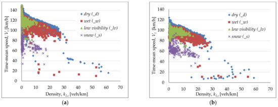
Figure 1.
Example of scatter graph of time mean speed vs. traffic density on the carriageway near Ljubljana in different traffic lanes: (a) lane 2—left (overtaking) lane; (b) lane 1—right lane.
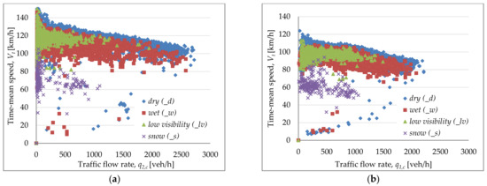
Figure 2.
Example of scatter graph of time mean speed vs. traffic flow rate on the carriageway near Ljubljana in different traffic lanes: (a) lane 2—left (overtaking) lane; (b) lane 1—right lane.
In any case, we found out from the literature review and experience with known events in unstable traffic flow that, at an increased total traffic flow rate qtot,c, the flow rate in the left lane q2,c is higher than in the right lane q1,c. This confirms the finding about the unused capacity of lane 1 (LFR2 > LFR1), where the speeds are lower [12,14,18]. It is also interesting to note that this difference varies depending on weather conditions [19], which means that it makes sense to consider it as a decision-making criterion in active traffic lane control. Differences in the traffic flow density ∆kc occurred at the maximum measured flows. In good weather conditions, the density was lower in lane 1 (k1 < k2), while it was lower in the overtaking lane (k2 < k1) in adverse weather conditions.
In addition to the above-mentioned traffic flow characteristics, we empirically analysed the remaining characteristics on the basis of the findings [15,43], which allowed us to perform a microsimulation in the next step to substantiate the appropriateness of the decision to not permit HGV to change traffic lanes.
Traffic Flow Speed Analysis
In order to further analyse the results and evaluate the measures taken to control HGVs, we also determined the empirical speed distribution functions of light and heavy vehicles at mentioned test sites near Ljubljana. We considered the vehicle categorisation of the current AHTMS, which groups vehicles into light and heavy vehicles [36]. At the same time, in the years before the COVID-19 pandemic, there were no special administrative limits or overtaking bans for HGVs. Figure 3a shows the results of the speed analysis for the example of test site 0178 for lane 2 for passenger cars (_pc), and Figure 3b for lane 1. Similar results are shown in Figure 3c,d for lanes 1 and 2 for heavy vehicles (_hv).
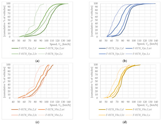
Figure 3.
Empirical speed distribution functions for different weather conditions at test site 0178: (a) passenger cars in lane 2; (b) passenger cars in lane 1; (c) heavy vehicles in lane 2; (d) heavy vehicles in lane 1.
For test site 0865 in the Vipava Valley, we also investigated the influence of wind on the speed V of all vehicles (Figure 4). We determined four empirical distribution functions of speed V as a function of four types of AHTMS measures with respect to wind strength for traffic lane i. Wind strength was expressed not by the magnitude of some other statistical characteristic value (e.g., the maximum speed of wind gusts), but by the traffic management measure Zi for a specific vehicle category [36]. Z0 means that the wind does not require any special traffic management measures. An example of speed analysis for test point 0865 is shown in Figure 4. Nevertheless, in brackets, we still present the informative values of maximum wind gust speeds for individual bans or traffic management measures [44]:
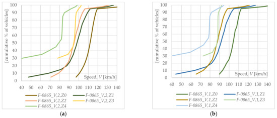
Figure 4.
Empirical speed distribution functions with different traffic management measures in the case of wind at test point 0865: (a) lane 2—left (overtaking) lane; (b) lane 1—right lane.
- Z1: exclusion for camper vans, refrigerator vehicles, and sheeted vehicles with the MAM of 8 t (wind from 80 km/h to 99 km/h);
- Z2: exclusion for camper vans, all sheeted vehicles, and refrigerator vehicles (wind from 100 km/h to 129 km/h);
- Z3: exclusion for camper vans, all Z2 level vehicles, and buses (wind from 130 km/h to 149 km/h);
- Z4: ban for all vehicles—road closure (wind over 150 km/h).
In the case of measure Z4, the highway is closed for all vehicles, which means that only light passenger cars that leave the traffic network and are not yet familiar with traffic control measures are subject to speed measurements. If wind gust speeds exceed a certain level with a simultaneous increase in wind strength and vice versa, highway or expressway traffic is regulated in accordance with the decision of the supervisory group of the traffic operators. If a negative trend occurs, the ban is lifted. Each such turn takes up to 2 h.
In the case of extreme winds, heavy traffic is excluded or the road is closed; hence, this generally does not affect the highway capacity utilisation. Thus, we did not consider the influence of wind on a possible measure of the truck overtaking ban.
3. Modelling the Efficiency of Traffic Lane Control and Weather Conditions
A hypothetical simulation model was created in the PTV Vissim software environment. Using the Wiedemann 99 traffic model, we set up a 2 km long unidirectional highway carriageway link. The scheme is shown in Figure 5, where the positions of the cross-sections P1 and P2 are marked, along with the virtual simulation test points, such as sensor loops {K1, K2, K3, K4} on the individual traffic lanes corresponding to the individual traffic lane i = {1—right lane; 2—left (overtaking) lane} and measuring points {K5, K6} on the carriageway. The measuring points at the cross-sections were used to observe the lane distribution of traffic flow. The first 600 m of the model was intended to establish a stable traffic flow, the next 1200 m was intended for measurements, and another 200 m was intended for exit vehicles from the simulation model of the road network. In the section between P1 and P2, there were link control sensors T1 and T2 on each lane, from which we obtained the values of traffic flow characteristics on the 1000 m long section, separately by traffic lanes and for the “average” lane. The “average” lane represents the average value of the simulation results of both traffic lanes. In the selected microsimulation model, traffic flow is distributed among traffic lanes on the basis of parameters describing the behaviour of drivers and the characteristics of vehicles entering the simulation model. In order to use the model in a real environment, one should calibrate the model and make a comparison between the actual characteristics of the traffic flow and the modelled characteristics.
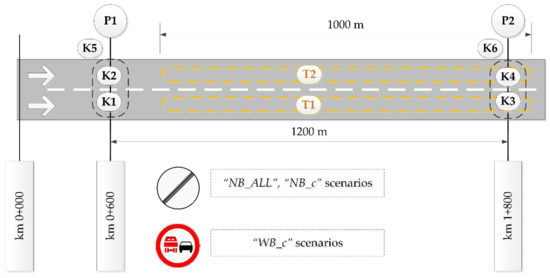
Figure 5.
Schema of unidirectional carriageway in the simulation traffic model.
The traffic model simulation time was Ts = 60 min and we gradually loaded the model in 10 min time intervals with different values of the flow rate of all vehicles on the carriageway. The total traffic flow rate increased uniformly at each interval qtot,c = {1500 veh/h, 2000 veh/h, 2500 veh/h, 3000 veh/h, 3500 veh/h, 4000 veh/h}. We modelled the situation in which LFR2,c ≈ LFR1,c occurs in the traffic flow, i.e., in the case in which vehicles change lanes intensively and both traffic lanes are approximately equally loaded. This was observed through the viewer interface and control points (Figure 5 and Figure 6a,b). In the simulation, we considered the constant share of heavy vehicles Phv = 10%.
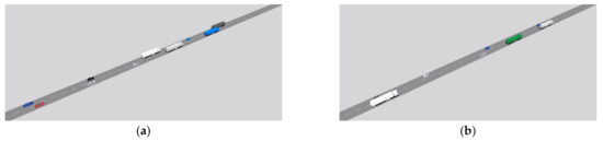
Figure 6.
Example of uniform traffic flow distribution across traffic lanes: (a) NB_ scenario; (b) WB_ scenario.
We modelled three scenarios, two of them for six weather conditions:
- Without traffic control restrictions and without separate consideration of weather conditions c; “ALL” weather conditions are considered—NB_ALL simulations (Figure 6a);
- Without traffic control restrictions, but with weather conditions c considered—NB_c simulations (Figure 6a):
- NB_d simulation taking into account the empirical speed distribution functions of light (F-0178,Vpc,i,d) and heavy vehicles (F-0178,Vhv,i,d), in traffic lanes i = {1, 2}, in “dry” and fair weather (Figure 3);
- NB_w1-, NB_w2-, NB_w3 simulation by taking into account the empirical speed distribution functions of light (F-0178,Vpc,i,wi) and heavy vehicles (F-0178,Vhv,i,wi), in traffic lanes with different precipitation intensities and wetness of road surface (Figure 3);
- NB_lv simulation by taking into account the empirical speed distribution function of light (F-0178,Vpc,i,lv) and heavy vehicles (F-0178,Vhv,i,lv) in traffic lanes with “poor visibility” (Figure 3);
- NB_s simulation by taking into account the empirical speed distribution function of light (F-0178,Vpc,i,s) and heavy vehicles (F-0178,Vhv,i,s) in traffic lanes under “winter conditions” (Figure 3);
- With the traffic control of “overtaking ban for HGVs”, but with consideration of road-weather conditions c—WB_c simulations (Figure 6b): {WB_d, WB_w1, WB_w2, WB_w3, WB_lv, WB_s}. The road-weather conditions were determined parametrically using the corresponding empirical speed distribution functions of light and heavy vehicles as presented in the previous section.
In total, we performed 13 different simulation cases and each case included five iterations, yielding a total of 65 simulated cases. While there were many iterations of different scenarios simulations, the average values of the results are discussed in Section 4.
4. Results and Discussion
This section presents the results of traffic flow simulation using a microscopic traffic model for a case of three scenarios of traffic lane control with various weather and traffic conditions. The simulation results of the first scenario represent a reference value without considering weather conditions and considering the speed distribution function for the “average” lane. Then, two scenarios follow with knowledge of the lane speed distribution function of different vehicles in different weather conditions, and the third with the measure of “overtaking ban for HGVs”, which can be used to reduce the instability of the traffic flow. In this way, faster vehicles are separated from slower ones, resulting in greater speed homogeneity of traffic flow in each traffic lane. For each simulated case, the relative delays rD,Sc were determined [45]. For the specific simulation scenario Sc = {NB_ALL, NB_c, WB_c}, the line graphs in Figure 7a,b show the total relative delay rD,Sc as a function of traffic flow density kSc, which we ensured to be nearly identical for all compared cases.
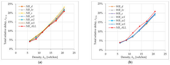
Figure 7.
Total relative delays of vehicles in the “average” lane depending on the traffic flow density for simulation scenarios: (a) NB_ALL, NB_c; (b) NB_ALL, WB_c.
In Table 1, the relative delay differences between rD,NB_ALL and rD,NB_c (rD,NB_ALL − rD,NB_c) and between rD,NB_d and rD,NB_c (rD,NB_d − rD,NO_c) were added to delays rD,Sc. Table 2 shows the results of relative delays and differences between rD,NB_ALL and rD,WB_c (rD,NO_ALL − rD,WB_c) and between rD,WB_d and rD,WB_r (rD,WB_d − rD,WB_c). In Table 1, we compared the difference in total relative delays between the scenario that assumes no special traffic lane control and considers the input parameters determined without considering the weather conditions (reference simulation NB_ALL) and the simulation scenarios that consider different weather conditions (simulations NB_c). In Table 2, we compared the difference with the scenario that assumes a traffic management measure. Both tables also show the relative delay difference with respect to dry weather conditions rD,NB_d and rD,WB_d (simulations NB_d and WB_d).

Table 1.
Relative delays of vehicles depending on traffic density for simulation scenarios NB_ALL and NB_c, along with relative differences for the “average” lane.
Table 2.
Relative delays of vehicles depending on traffic density for simulation scenarios NB_ALL and WB_c, along with relative differences for the “average” lane.
The graph in Figure 7a shows that the total relative delay rD,Sc was higher than the reference value when considering weather conditions and knowing the distribution of the traffic flow rate in lanes. When comparing the average values (kSc ≈ 13.0 veh/km), the relative delays were 2% to 12% higher in all cases (Table 1); however, at the approximate value of traffic flow density of 12 veh/km, this difference decreased again. The differences were similar for all simulation scenarios in the same size class up to a density of 14 veh/km. At maximum traffic flow rate and density of just over 20 veh/km, which we simulated in the sixth time interval, relative delays increased again to 1% in dry weather conditions, from 3% to 5% in wet conditions, to 8% in poor visibility, and up to 12% in snowy conditions. Generally, results of the paired t-test indicated that there is a non-significant medium difference between rD,NB_ALL (µ = 11.4, σ = 6.4) and rD,NB_d (µ = 11.6, σ = 6.4), t = 1.9, p = 0.060. Otherwise there is a significantly large difference between rD,NB_ALL and non rD,NB_d, e.g., rD,NB_S (µ = 12.7, σ = 7.1), t = 3.5, p = 0.009.
The graph in Figure 7b presents rD,Sc as a function of traffic flow density for the scenario without special traffic management measures (NB_ALL) and with the measure “overtaking ban for HGVs” (WB_c), but with knowledge of the lane speed distribution functions for different weather conditions and different vehicles. Regardless of traffic flow density, traffic control reduced rD,Sc by an average of 9% to 13% considering the weather conditions (Table 2). Differences in relative delays between different weather conditions appeared with increasing traffic density and with the same traffic control measure. It is interesting to note that rD,Sc did not deviate significantly from the reference value up to the value of the traffic flow density kSc ≤ 9 veh/km, which we interpreted as a lower efficiency of the traffic management measure. For the cases kSc > 9 veh/km, the differences increased and reached values from −19% to −24%, with the greatest impact in dry weather conditions. Thus, for a traffic flow density of around 9 veh/km, the relative reduction in total relative delays without and with lane management was up to 1% in heavy rainfall and up to 4% in light rain and in dry conditions. With the additional increase in traffic flow density, the relative differences according to weather conditions no longer changed with the same trends. With a traffic flow density of about 21 veh/km and with the WB_c measure, the total relative delays were reduced by 8% to 9% in all weather conditions, and by 5% in snow. Again, results of the paired t-test indicated that there is a significantly large difference between rD,WB_c (µ = 10.1, σ = 5.4) and rD,NB_ALL (µ = 11.4, σ = 5.8), n = 36, t = 8.2, p < 0.001.
The criterion of traffic control on highways when traffic flow is becoming unstable is usually determined by the total equivalent flow rate qe,tot,ALL and the equivalent flow rate in the overtaking lane qe,2,ALL, as well as the standard deviation of speed in the overtaking lane [34,36]. Similarly, the total equivalent flow rate qe,tot,ALL and the proportion of heavy vehicles Phv determine the criterion for traffic management in the case of traffic instability at a large share of heavy vehicles. Considering that free-flow speed varies depending on weather conditions, in the case where the traffic flow rate is a criterion for traffic management, different threshold values of the flow rate threshold should be taken into account, depending on weather and traffic conditions. Therefore, this article demonstrates that it is reasonable to further investigate the effectiveness of the current AHTMS criteria and possibly establish new criteria for traffic management in the case of instability by using other traffic flow characteristics, such as the Coefficient of Variation of Speed CVS [30,46], the traffic flow density kc, or the possibility of changing lanes depending on environmental factors [19]. For comparison, on the basis of the simulation, we calculated the total delays of all vehicles pD,Sc on the simulation model road network, varying the input data and calculating the equivalent traffic flow rate for the case of a highway level terrain according to the HCM methodology [17]. The graph in Figure 8a shows total delays pD,Sc as a function of the total equivalent traffic flow rate qe,tot,Sc for the scenario without special traffic management (NB_c), and that in Figure 8b shows the same scenario with the simulated measure “overtaking ban for HGVs” (WB_c). In both cases, the results of the NB_ALL scenario are also shown as a reference red polyline.
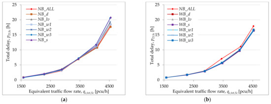
Figure 8.
Simulated total delays of all vehicles as a function of total equivalent traffic flow rate: (a) for NB_ALL, NB_c scenarios; (b) for NB_ALL, WB_c scenarios.
In addition to the results, Table 3 shows the relative differences, expressed by the index ratio , where pD,NB_ALL represents the total delays of the vehicles in the reference simulation. In the range of flow rates from 1500 pcu/h to about 2300 pcu/h, delays under bad weather conditions were lower than under reference conditions, except for dry weather conditions. This difference may be a result of adverse weather conditions that reduced the speed of vehicles and changed the lane distribution in some way [19]. The ratio value changed with the next step of the traffic flow rate increase. In the qe,tot,Sc interval between 2300 pcu/h and 3500 pcu/h, delays were again shorter. With better weather conditions, the differences over the flow rate value of around 2900 pcu/h decreased. At a flow rate of 3500 pcu/h, the delay differences only increased and no longer fluctuated. At the end of the simulation, total delays increased by 16% in winter conditions, 15% in heavy rain, 8% in moderate rain, and up to 3% in light rain. In dry conditions, a 1% improvement over the reference value was observed.
Table 3.
Total delays in simulated network depending on qe,tot,Sc for simulation scenarios NB_ALL and NB_c, along with index ratios.
The line graph in Figure 8b presents pD,Sc as a function of qe,tot,Sc for the scenario with the simulated measure “overtaking ban for HGVs” (WB_c scenarios). In all cases, delays were lower with the traffic control; however, in the qe,tot,Sc interval from 1500 pcu/h to 2900 pcu/h, this difference was not as pronounced as at higher flow rates. In Table 4, in addition to the results on total delays, we present the relative difference, expressed by indices and , where pD,NB_ALL is the total vehicle delay of the reference simulation, pD,NB_c is the total delay without traffic control, and pD,WB_c is the total delay with the traffic control measure in different weather conditions c. Owing to the “overtaking ban for HGVs”, delays were 2% to 3% lower in fair weather conditions and 5% to 7% lower in adverse weather conditions. With higher traffic flow rates, delays could be reduced by up to 21%, regardless of weather conditions, but only up to a certain threshold. As rates exceeded 4500 pcu/h, the relative differences between the delays under different conditions decreased. From the results, similar to the case of relative delays, it appears that traffic management with truck overtaking bans at lower flow rates was not as effective as at flows above 2800 pcu/h.
Table 4.
Total delays in simulated network depending on qe,tot,Sc for simulated scenarios NB_ALL and WB_c, along with index ratios.
Through traffic simulations, we confirmed that relative traffic delays depend on road weather conditions. In adverse conditions, these were, on average, 1% to 10% higher than relative delays in dry conditions with the same traffic flow rate, and worst in the case of winter conditions, followed by low visibility and various rain intensities or wetness. For the maximum simulated flow rate of 4000 veh/h with a 10% share of heavy vehicles, i.e., a traffic flow density of slightly more than 20 veh/km, when the characteristics of the traffic flow in the traffic lanes were known, the relative delays were 1% greater in dry weather conditions, 3% to 5% greater in wet conditions, 8% greater in poor visibility, and up to 12% greater in winter conditions than in the case where the traffic flow characteristics were determined independently of weather conditions (_ALL). By simulating the traffic management measure of the truck overtaking ban, we calculated that relative delays were reduced by an average of 15% to 18% compared to a benchmark without traffic management. The largest difference occurred with medium-sized flow rates or a density of about 12 veh/km and was as high as 25% in snowy weather conditions. We found that the effect of traffic management was greater in the case of adverse weather conditions with the same traffic demand. The relative difference varied depending on the density of traffic flow. Traffic management had the greatest effect in the case of medium density (about 12 veh/km), where the relative differences between weather conditions were small. We also calculated total delays as a function of the equivalent flow rate. In all weather conditions, traffic management could achieve lower delays; however, in the interval of flows from 1500 pcu/h to 2900 pcu/h, this difference was not as large as at higher flow rates. Owing to traffic management, delays were reduced by 2% to 3% in good weather conditions and by 5% to 7% in adverse weather conditions. However, at higher flow rates, delays could be reduced by up to 21%, regardless of weather conditions, but only up to a certain limit. When traffic flow rates exceeded 4500 pcu/h, the relative differences between delays under different conditions decreased. Similar to the case of relative delays, the results show that traffic management with truck overtaking bans at lower traffic demand was not as effective as for flow rates above 2300 pcu/h with a 10% share of heavy vehicles. Total delays may be equal to or even lower in the case of rain or a wet carriageway. We found that truck overtaking bans had a positive effect when considering the relative difference in total delays but only when the traffic flow rate of all vehicles and heavy vehicles on the carriageway separately exceeded a certain threshold value. As part of our research, we limited the proportion of HGVs in the total flow rate. If we were to vary this, we would achieve more results. With the research, we proved that sensing weather conditions is important in the case of decision-making for lane traffic control.
5. Conclusions
The research presented in this article included an analysis of traffic flow characteristics in different highway traffic lanes with an emphasis on the influence of weather conditions. With the results of the analyses, we confirmed that weather conditions have different effects on traffic flow and lane distribution. This may be important when monitoring capacity utilisation and other performance criteria of highway traffic control services for the future. In general, we found that, in certain cases, bad weather has a positive effect on the homogeneity of the traffic flow speed and that, under such circumstances, vehicles do not change lanes, which can reduce delays.
Using a traffic microsimulation on a highway section, we determined vehicle delays as a function of traffic demand in different weather conditions using the example of the traffic management scenario “overtaking ban for HGVs”. The delays calculated with the traffic model were compared with a reference scenario without traffic management in simulated different weather conditions but with controlled traffic input data. If the effectiveness of the AHTMS measures is measured by the reduction in delays, it would be important to know the result that the same value of delay is achieved for different values of traffic flow density in different weather situations. In practice, the techniques for empirically determining delays can be complex; hence, we can expect the introduction of online traffic models soon.
Of course, it would be interesting to investigate whether it is justified to have a daytime truck overtaking ban independent of traffic flow rates on all highways and whether preference should be given to AHTMS, in which a measure of dynamic control of heavy vehicles would be implemented when needed, depending on traffic demand, in a real case and not hypothetically. We should know that in Slovenia, AHTMSs have already been implemented on highways and that Slovenia has the National Traffic Management Centre, whose functionality also includes the online modelling of traffic flows, including for short-term prediction. An overtaking ban for HGVs was established on the whole dual carriageway highway network in Slovenia in a static way (overtaking is permanent and intermittent on some highways). Through our research, we found that dynamic bans can be more effective when we include the dynamics of traffic demand and environmental conditions. At the same time, actual compliance with any strict rules should be investigated. The next issue related to the problem of homogenisation of traffic flows is certainly the monitoring and management of recreational vehicles, focusing on motorhomes and vehicles with tourist trailers, which have a maximum authorised speed that is different from other vehicles.
Author Contributions
Conceptualization, R.R., R.M. and I.S.; Data curation, R.R., R.M. and I.S.; Formal analysis, R.R., R.M. and I.S.; Funding acquisition, R.R.; Investigation, R.R. and R.M.; Methodology, R.R., R.M. and I.S.; Project administration, R.R. and I.S.; Resources, R.R. and R.M.; Software, R.R. and R.M.; Supervision, R.R. and I.S.; Validation, R.R., R.M. and I.S.; Visualization, R.R., R.M. and I.S.; Writing—original draft, R.R. and R.M.; Writing—review & editing, R.R., R.M. and I.S. All authors have read and agreed to the published version of the manuscript.
Funding
This research received no external funding.
Institutional Review Board Statement
Not applicable.
Informed Consent Statement
Not applicable.
Data Availability Statement
The data presented in this study are available on request from the corresponding authors.
Acknowledgments
The authors would like to thank the Slovenian Infrastructure Agency (DRSI) and the Motorway Company of the Republic of Slovenia (DARS d.d.) for their cooperation and access to traffic and environmental data from their information systems.
Conflicts of Interest
The authors declare no conflict of interest.
References
- Barcelo, J. Models, Traffic Models, Simulation, and Traffic Simulation. In Fundamentals of Traffic Simulation; International Series in Operations Research & Management Science; Springer: Berlin/Heidelberg, Germany, 2010; Volume 145, pp. 1–62. [Google Scholar]
- De Oliveira, L.B.; Camponogara, E. Multi-Agent Model Predictive Control of Signaling Split in Urban Traffic Networks. Transp. Res. Part C Emerg. Technol. 2010, 18, 120–139. Available online: https://www.sciencedirect.com/science/article/pii/S0968090X09000540 (accessed on 2 September 2022). [CrossRef]
- Steinhoff, C.; Keller, H.; Kates, R.; Farber, B. Driver Perceptions of the Effectiveness of VMS. In Proceedings of the 7th World Congress on Intelligent Transport Systems, Turin, Italy, 6–9 November 2000. [Google Scholar]
- Sándor, Z. Effects of Weather Related Safety Messages on the Motorway Traffic Parameters. Period. Polytech. Transp. Eng. 2017, 45, 58–66. Available online: https://pp.bme.hu/tr/article/view/9117 (accessed on 2 September 2022). [CrossRef]
- van Nes, N.; Brandenburg, S.; Twisk, D. Improving Homogeneity by Dynamic Speed Limit Systems. Accid. Anal. Prev. 2010, 42, 944–952. Available online: https://www.sciencedirect.com/science/article/pii/S0001457509000992 (accessed on 2 September 2022). [CrossRef]
- Hidas, P. Modelling Lane Changing and Merging in Microscopic Traffic Simulation. Transp. Res. Part C Emerg. Technol. 2002, 10, 351–371. Available online: https://www.sciencedirect.com/science/article/pii/S0968090X02000268 (accessed on 2 September 2022). [CrossRef]
- Sun, K.; Zhao, X.; Wu, X. A Cooperative Lane Change Model for Connected and Autonomous Vehicles on Two Lanes Highway by Considering the Traffic Efficiency on Both Lanes. Transp. Res. Interdiscip. Perspect. 2021, 9, 100310. Available online: https://www.sciencedirect.com/science/article/pii/S2590198221000178 (accessed on 2 September 2022). [CrossRef]
- Hoseini, S.M.S. Comparison of Microscopic Drivers’ Probabilistic Lane-Changing Models with Real Traffic Microscopic Data. Promet. Traffic Transp. 2011, 23, 241–251. [Google Scholar] [CrossRef]
- Wall, G.; Hounsell, N. Microscopic Modeling of Motorway Diverges. Eur. J. Transp. Infrastruct. Res. 2005, 5, 139–158. [Google Scholar]
- Heidemann, D. Distribution of Traffic to the Individual Lanes on Multilane Unidirectional Roadways. In Proceedings of the Second International Symposium on Highway Capacity, Sydney, Australia, August 1994; Australian Road Research Board: Vermont South, Australia; Transportation Research Board: Washington, DC, USA, 1994; Volume 1, pp. 265–276. [Google Scholar]
- Li, L.; Wang, F.-Y. The Automated Lane-Changing Model of Intelligent Vehicle Highway Systems. In Proceedings of the IEEE 5th International Conference on Intelligent Transportation Systems, IEEE, Singapore, 6 September 2002; pp. 216–218. [Google Scholar]
- Wu, N. Equilibrium of Lane Flow Distribution on Motorways. Transp. Res. Rec. 2006, 1965, 48–59. Available online: https://journals.sagepub.com/doi/pdf/10.1177/0361198106196500106 (accessed on 2 September 2022). [CrossRef]
- Daganzo, C.F. A Behavioral Theory of Multi-Lane Traffic Flow. Part I: Long Homogeneous Freeway Sections. Transp. Res. Part B Methodol. 2002, 36, 131–158. [Google Scholar] [CrossRef]
- Pompigna, A.; Rupi, F. Lane-Distribution Models and Related Effects on the Capacity for a Three-Lane Freeway Section: Case Study in Italy. J. Transp. Eng. Part A Syst. 2017, 143, 05017010. Available online: https://ascelibrary.org/doi/10.1061/JTEPBS.0000080 (accessed on 2 September 2022). [CrossRef]
- Farooq, D.; Juhasz, J. Simulation-Based Analysis of the Effect of Significant Traffic Parameters on Lane Changing for Driving Logic “Cautious” on a Freeway. Sustainability 2019, 11, 5976. [Google Scholar] [CrossRef]
- Grabec, I.; Kalcher, K.; Švegl, F. Modeling and Forecasting of Traffic Flow. Nonlinear Phenom. Complex Syst. 2010, 13, 53–63. [Google Scholar]
- Transportation Research Board. Highway Capacity Manual 6th Edition: A Guide for Multimodal Mobility Analysis; The National Academies Press: Washington, DC, USA, 2016. [Google Scholar]
- Xiao, C.; Shao, C.; Meng, M.; Wang, P.; Wang, B. Lane Flow Distribution of a Long Continuous Highway. Int. J. Transp. Econ. Eng. Law 2014, 56, 1–16. [Google Scholar]
- Rijavec, R.; Šemrov, D. Effects of Weather Conditions on Motorway Lane Flow Distributions. Promet. Traffic. Traffico 2017, 30, 83–92. Available online: https://traffic.fpz.hr/index.php/PROMTT/article/view/2521 (accessed on 2 September 2022). [CrossRef]
- Haug, A.; Grosanic, S. Usage of Road Weather Sensors for Automatic Traffic Control on Motorways. Transp. Res. Procedia 2016, 15, 537–547. Available online: https://www.sciencedirect.com/science/article/pii/S2352146516305774 (accessed on 2 September 2022). [CrossRef]
- Calvert, S.; Snelder, M. Influence of Weather on Traffic Flow: An Extensive Stochastic Multi-Effect Capacity and Demand Analysis. In European Transport/Trasporti Europei; Institute for Transport Studies in the European Economic Integration: Trieste, Italy, 2016; Volume 60, pp. 1–24. [Google Scholar]
- Weng, J.; Liu, L.; Rong, J. Impacts of Snowy Weather Conditions on Expressway Traffic Flow Characteristics. Discrete Dyn. Nat. Soc. 2013, 2013, 791743. Available online: https://downloads.hindawi.com/journals/ddns/2013/791743.pdf (accessed on 2 September 2022). [CrossRef]
- Aaheim, H.A.; Hauge, K.E. Impacts of Climate Change on Travel Habits—A National Assessment Based on Individual Choices; CICERO Center for International Climate and Environmental Research: Oslo, Norway, 2005. [Google Scholar]
- Skvarča, S. Impact of Weather on Traffic Flow Characteristics. Bachelor’s Thesis, University of Ljubljana, Ljubljana, Slovenia, 2013. (In Slovenian). [Google Scholar]
- Kršmanc, R. Road Surface Condition Forecasting from Historical Data and Weather Forecast. Ph.D. Thesis, University of Ljubljana, Ljubljana, Slovenia, 2013. Available online: http://eprints.fri.uni-lj.si/2109/1/Krsmanc1.pdf (accessed on 2 September 2022). (In Slovenian).
- Rudloff, C.; Leodolter, M.; Bauer, D.; Auer, R.; Brög, W.; Knud, K. Influence of Weather on Transport Demand: A Case Study from the Vienna Region. In Proceedings of the Transportation Research Board (TRB) 94th Annual Meeting, Washington, DC, USA, 11–15 January 2015. [Google Scholar]
- Billot, R.; El Faouzi, N.-E.; De Vuyst, F. Multilevel Assessment of the Impact of Rain on Drivers’ Behavior. Transp. Res. Rec. J. Transp. Res. Board 2009, 2107, 134–142. Available online: https://journals.sagepub.com/doi/10.3141/2107-14 (accessed on 2 September 2022). [CrossRef]
- Hablas, H.E. A Study of Inclement Weather Impacts on Freeway Free-Flow Speed by a Study of Inclement Weather Impacts on Freeway Free-Flow Speed. Master’s Thesis, Virginia Polytechnic Institute and State University, Blacksburg, VA, USA, 2007; p. 112. [Google Scholar]
- Ibrahim, A.T.; Hall, F.L. Effect of Adverse Weather Conditions on Speed–Flow Occupancy Relationships. Transp. Res. Rec. 1994, 1457, 184–191. [Google Scholar]
- Huzjan, B.; Mandžuka, S.; Kos, G. Real-Time Traffic Safety Management Model on Motorways. Teh. Vjesn. Tech. Gaz. 2017, 24, 1457–1469. Available online: https://hrcak.srce.hr/188243 (accessed on 2 September 2022).
- Duret, A.; Ahn, S.; Buisson, C. Lane Flow Distribution on a Three-Lane Freeway: General Features and the Effects of Traffic Controls. Transp. Res. Part C Emerg. Technol. 2012, 24, 157–167. Available online: https://www.sciencedirect.com/science/article/pii/S0968090X12000307 (accessed on 2 September 2022). [CrossRef]
- Lee, J.; Park, B.B. Lane Flow Distributions on Basic Segments of Freeways Under Different Traffic Conditions. In Proceedings of the Transportation Research Board 89th Annual Meeting, Washington, DC, USA, 10–14 January 2010; Transportation Research Board: Washington, DC, USA, 2010. [Google Scholar]
- Sabir, M. Weather and Travel Behaviour. Ph.D. Thesis, VU University, Amsterdam, The Netherlands, 2011. [Google Scholar]
- BASt. Technische Lieferbedingungen Für Streckenstationen; TLS 2012; Bundesanstalt für Straßenwesen (BASt): Bergisch Gladbach, Germany, 2012; Available online: https://www.bast.de/DE/Publikationen/Regelwerke/Verkehrstechnik/Unterseiten/V5-tls.html (accessed on 2 September 2022).
- Nagy, E.; Sándor, Z. Overtaking Ban for Heavy Goods Vehicle in Hungary on the National Motorway Network. Pollack Period. 2012, 7, 83–95. [Google Scholar] [CrossRef]
- DARS. Guidelines for the Traffic Control System on Highways in the Republic of Slovenia; DARS: Celje, Slovenia, 2004. [Google Scholar]
- European Commision. EasyWay Harmonising European ITS Services and Actions, Traffic Management Services, HGV OVERTAKING BAN, Deployment Guideline (TMS-DG06) v 2.0; Alain, R., Ed.; European Commision (DG MOVE): Brussels, Belgium, 2012. [Google Scholar]
- Hardman, E.; Morris, B.; Owlett, P.; Rees, T. Directorate General for Internal Policies, Policy Department B Structural and Cohesion Policies, Transport and Tourism: The Impact of Overtaking Bans for HGVs on Two-Lane Highways, on Traffic Flow and Routes of Transport; TRL Limited: Brussels, Belgium, 2010; Available online: https://www.europarl.europa.eu/thinktank/en/document/IPOL-TRAN_NT(2010)431607 (accessed on 2 September 2022).
- Schengen: A Guide to the European Border-Free Zone. Available online: https://www.europarl.europa.eu/news/en/headlines/security/20190612STO54307/schengen-a-guide-to-the-european-border-free-zone (accessed on 6 September 2022).
- Neuburger, L.; Egger, R. Travel Risk Perception and Travel Behaviour during the COVID-19 Pandemic 2020: A Case Study of the DACH Region. Curr. Issues Tour. 2021, 24, 1003–1016. [Google Scholar] [CrossRef]
- DRSI Slovenian Infrastructure Agency. Road Traffic Loads Since 1997. In Open Data of Slovenia 2020. Available online: https://podatki.gov.si/dataset/pldp-karte-prometnih-obremenitev (accessed on 2 September 2022).
- Kyte, M.; Khatib, Z.; Shannon, P.; Kitchener, F. Effect of Environmental Factors on Free-Flow Speed. In Proceedings of the 4th International Symposium on Highway Capacity, Maui, HI, USA, 27 June–1 July 2000; pp. 108–119. [Google Scholar]
- Chen, C.; Zhao, X.; Liu, H.; Ren, G.; Zhang, Y.; Liu, X. Assessing the Influence of Adverse Weather on Traffic Flow Characteristics Using a Driving Simulator and VISSIM. Sustainability 2019, 11, 830. [Google Scholar] [CrossRef]
- Traffic Information Centre for Public Roads Wind Measuring System Burja (Vipava Valley). Available online: https://www.promet.si/en/burja-wind (accessed on 6 September 2022).
- PTV Group. PTV Vissim 2022 User Manual; PTV Group: Karlsruhe, Germany, 2022; p. 1378. [Google Scholar]
- Grumert, E.F.; Tapani, A.; Ma, X. Characteristics of Variable Speed Limit Systems. Eur. Transp. Res. Rev. 2018, 10, 21. [Google Scholar] [CrossRef]


Publisher’s Note: MDPI stays neutral with regard to jurisdictional claims in published maps and institutional affiliations. |
© 2022 by the authors. Licensee MDPI, Basel, Switzerland. This article is an open access article distributed under the terms and conditions of the Creative Commons Attribution (CC BY) license (https://creativecommons.org/licenses/by/4.0/).