Optimization and Performance Analysis of a Distributed Energy System Considering the Coordination of the Operational Strategy and the Fluctuation of Annual Hourly Load

Abstract

The operation strategies of a distributed energy system (DES) are usually proposed according to the electrical load (FEL) and the thermal load (FTL), which take the cooling/heating load or electric load as unique constraint conditions that result in a too high or too low equipment load rate. This paper proposes a new hybrid operation strategy (HOS) that takes the full utilization of natural gas and the minimization of power consumption from the power grid as constraints and coordinates the cooling/electricity ratio and heating/electricity ratio of buildings and equipment. In the optimization phase of a DES, an optimization method based on the discretization of the load is proposed to investigate the influence of the uncertainty of the load on the DES, which helps to avoid repeated load simulations and provides stronger adjustability by quoting the normal distribution function to obtain multiple sets of load data with different fluctuations. Further, a multi-objective optimization model combining the genetic algorithm (GA) and mixed integer linear programming algorithm (MILP) was established to find the optimal configuration of equipment capacities by comprehensively considering the annual total cost, carbon emissions, and energy efficiency of the DES. Finally, an office building example was used to validate the feasibility of the above theories and methods. Compared with the FEL and FTL, the HOS reduced the energy waste of the DES by 19.7% and 15.5%, respectively. Compared with using a typical daily load, using an annual hourly load to optimize the DES-HOS produced a better comprehensive performance and lower adverse impacts derived from load fluctuations.

1. Introduction

It is imperative to develop clean energy and energy conservation technology as a result of the scarcity of fossil fuels and the related environmental problems [1]. Along with the continuing growth of carbon dioxide emissions generated by the energy consumption of buildings, the distributed energy system (DES) has received much attention in terms of reducing energy consumption, increasing renewable energy utilization, and enhancing energy reliability. The DES is an energy supply system with many multiple synonymous names, such as the hybrid renewable energy system (HRES) [2], combined cooling heating and power (CCHP) [3], and the integrated energy system (IES) [4]. In this paper, the acronym DES is used. Compared with the separate energy system (SP), the DES can integrate a variety of clean energy sources, such as natural gas [5], solar energy [6], wind energy [7], biomass energy [4], and other energies to provide cooling, heating, and power for users. The advantages of the DES include financial savings, reduced emissions, improved system reliability, reduced pollution, and flexible operation [8,9]. Therefore, DES is more and more widely used.

The DES contains a variety of equipment, which simultaneously meet the needs of various energy loads, such as cooling, heating, and power [10,11]. In addition, a variety of energy supply models and operational strategies can be used to improve performance [12,13]. Therefore, astute design and optimization act to save costs, decrease fossil energy consumption, and reduce carbon emissions in the lifecycle of the building [11]. Common optimization algorithms include programming algorithms and intelligent algorithms. Vaccari et al. [14] presented a multi-objective optimization strategy to balance the profit and energy costs of a chemical plant with the aim of best managing the production rates of various products to fulfill a sales plan organized to satisfy numerous client requests. Liu et al. [15] established a DES that combined electric vehicles (EV) and hybrid energy storage (HES) to improve energy saving and emission reduction efficiency and reduce system investment operating costs. Huang et al. [16] proposed a mixed integer optimization model by designing a continuation method for integer decision variables and a constraint strategy with double penalties to ensure that the optimal start/stop states and operating power level of the distributed units were accurately configured under the premise of completely consuming renewable energy. Guo et al. [17] proposed a novel distributed energy system combining hybrid energy storage and system optimization configuration, simultaneously considering the operational strategy and a two-layer collaborative optimization method including energy efficiency, economy, and environmental protection. Huang et al. [18] revolutionized the idealized demand-side distribution and built an optimization model for a regional DES under discrete conditions. The optimization of the DES, which took the comprehensive cost as the objective function, determined the number, site, capacity of the energy station, and the optimal pipe network layout path from the energy station to the load center. Vaccari et al. developed an optimization tool for HRES based on a sequential linear programming (SLP) algorithm, which generates an operating plan over a specified time horizon of the setpoints of each device to meet all electrical and thermal load requirements with the minimum possible operating costs. The optimization of the DES may have a single extreme value or multiple extreme values owing to different constraints and assumptions. Programming algorithms have a higher accuracy and lower computational complexity when the optimization of the DES has a single extreme and clear constraints, but find it difficult to solve multi-extremum states, while intelligent algorithms are aimed at finding the global optimum of the multi-extremum problem as much as possible. In addition, the performance of a DES needs to be evaluated from economic, environmental, energy efficiency, and other perspectives, thus the multi-objective optimization algorithm can improve the performance of a DES more comprehensively than single objective strategies.

In the design phase of a DES, the operational strategy determines the operational mode of the DES equipment, thus it affects the selection and rated capacity of DES equipment. At present, a DES is usually optimized based on FEL and FTL, which has the advantages of reducing the complexity of DES optimization and operational management; however, this method is prone to cause unreasonable energy distributions and reduce energy efficiency [3,19]. Therefore, various researchers improved the operational strategies. Ma et al. [12] proposed the seasonal operational strategy (FSS), which could be seasonally adjusted by combining the cooling and heating ratio of the DES. Wu et al. [20] proposed a hybrid thermal and power operational strategy that switched operational modes according to the monthly cooling and thermal power load demand ratio. Yuan et al. [21] proposed a novel operational strategy utilizing system flexibility to schedule energy dispatch, which reduced dependence on the power grid and the underused fuel consumption, as compared with traditional FEL and FTL strategies. Although the above studies on operational strategies improve the performance of DES, the cooling/heating or power load is still used as the unique constraint to determine the load rate of the equipment, resulting in a too high or too low equipment load rate.

The load structure has an important influence on the optimization of a DES. Taking the data center as an example, its annual cooling/electricity ratio and heating/electricity ratio is highly stable and suitable for the energy supply of a DES [22,23]. It not only improves the economic efficiency and the energy efficiency of the system, but also improves the security of the power supply and reduces the dependence on the power grid [22,24]. However, in other scenarios, the load structure is often uncertain and fluctuates [25,26]. Robust optimization is a leading technology with which to solve uncertain problems. Li et al. [27] described the uncertainties of energy and time as a nonlinear bilevel robust optimization model, transforming them into a single-stage mixed integer linear problem for optimization and obtaining the optimal electricity and heat prices for interactions with each distributed energy system. Furthermore, other researchers adopted other methods to study the load structure. Huang et al. [18] constructed an optimization model to minimize the system cost under load discrete conditions, which is used to compare and analyze the annual cost under different load structure conditions. Lu et al. [28] employed a chance-constrained method to address the load uncertainty and transform the uncertain optimization into deterministic optimization. Their results show that increasing the confidence level resulted in a capacity increase in the waste heat boiler in heating mode. Liu et al. [29] proposed an optimal design method for the multi-energy complementary integrated energy system considering load uncertainties. Although these studies have optimized the DES considering the uncertainty of the load structure, the optimization of the DES that is based on the typical daily load in winter and summer ignores the fluctuation of the annual load of buildings, which leads to a deviation in optimization results from the optimal solution. In addition, the fluctuation studied by the extant load simulation method needs repeated simulations that involve constantly changing parameters, resulting in exorbitant calculation and strong randomness. Although researchers in relevant domains have realized that the fluctuation in the load has a negative impact on the performance of the DES, the existing methods are difficult to assess.

This paper aims to improve the comprehensive performance of the DES by improving the operational strategy and analyzing the impact of the annual load fluctuation on the DES-HOS. The hybrid operational strategy takes the full utilization of natural gas and the minimization of power consumption from the power grid as constraints to solve the problem of the unreasonable equipment load rate caused by existing operational strategies. In addition, a discretization method for the initial load uses the normal distribution function as the index function to obtain multiple sets of load with different volatilities, which avoids repeated load simulations and has a stronger adjustability. Further, the impact of load fluctuation on DES performance was analyzed through the optimization results based on discrete loads. To reduce the computational efficiency of the algorithm due to the excessive amount of load data, a multi-objective optimization algorithm is proposed by combining the GA algorithm and MILP algorithm. The optimization model includes an inner loop and outer loop, the outer loop functions to find the global optimal solution, while the inner loop improves the accuracy and reduces complexity. Finally, an office building was taken as an example to analyze the comprehensive performance of the DES under different operational strategies and load structures.

2. Model and Method

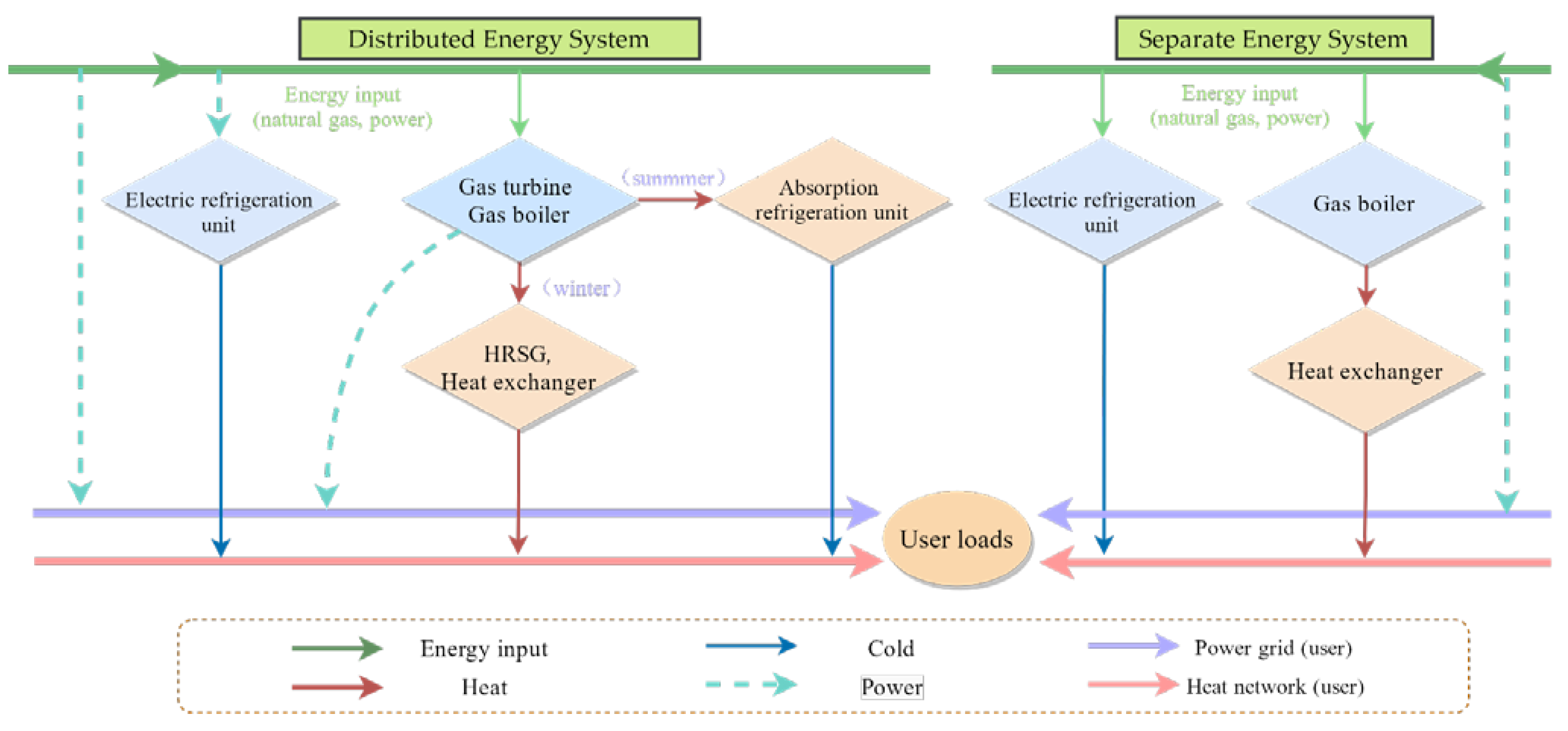
2.1. Operational Process and Structure

The structure of the DES and the separate energy system are shown in Figure 1. Typical, a DES is mainly composed of a power generation unit, a heat recovery steam generator (HRSG), a heat exchanger, an absorption refrigeration unit, and an electric refrigeration unit [18,30]. The DES uses the gas turbine as the power generation unit. The natural gas enters the gas turbine combustion chamber for combustion, producing high-temperature flue gas, which drives the turbine to generate power. The high-temperature flue gas discharged from the gas turbine can be recycled by the heat recovery steam generator and heat exchanger to recover waste heat in the winter and passes into the absorption refrigeration unit for refrigeration in the summer. If the energy generated by the gas turbine cannot meet the load of the building, the deficit energy is provided by the municipal power grid, the electric refrigerator unit, and the gas-fire boiler. The supply of cold, heat, and power can be made more reliable and flexible by coupling the various energy units mentioned above. In a typical separate energy system, the load demands are provided by the local utility grid, the gas boiler, and the electric cooling system, respectively [28].

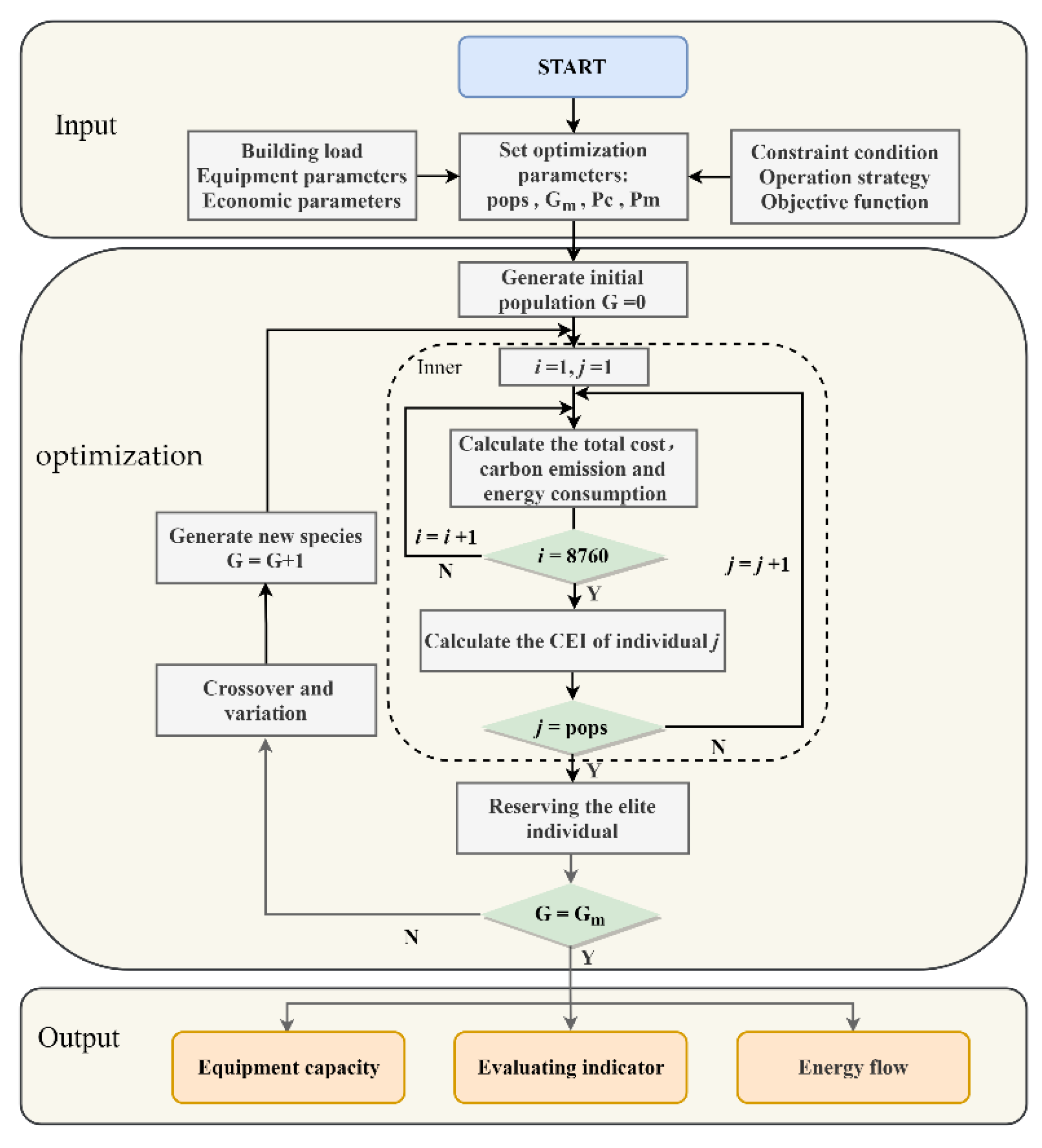
2.2. Process of Optimization

The optimization model includes the input layer, the optimization layer, and the output layer. In the input layer, the parameters of the building, equipment, and economics, the operational strategy, the objective function, and the constraint condition are input into the model. Furthermore, the parameters of optimization, which include the population size (pops), the maximum number of iterations (G_m), and the probabilities of crossover (Pc) and mutation (Pm), need to be set. The optimization layer consists of an outer loop, which generates the initial population and new populations of equipment capacities according to the parameters of optimization, and an inner loop, which calculates the annual cost, carbon emissions, and energy consumption of the DES and identifies the elite individual with optimal comprehensive performance [31]. Finally, the optimization results of equipment capacity, the evaluating indicator, and energy flow are output. The flow chart of the DES optimization model is shown in Figure 2.

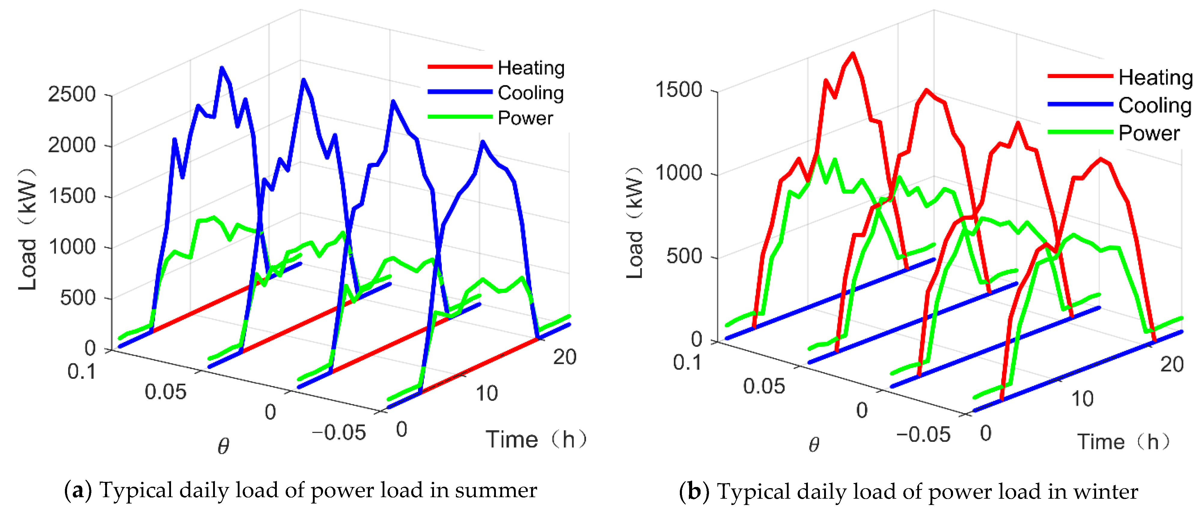
2.3. Load Calculation

The optimization of the DES based on a single set load cannot reflect the influence of the annual hourly load fluctuation on the optimization results. It is difficult to obtain multiple sets of annual hourly loads with different volatilities through the existing methods. Therefore, the discretization method is used to solve this problem. In addition, the variance of the annual load is quoted to describe the fluctuation. Finally, the typical daily load of the discrete load is obtained using a clustering algorithm. The specific steps are as follows:

Step 1: The type, location, heat transfer coefficient of the maintenance structure, and the structure of the building are obtained to calculate the initial cooling, heating, and power loads by DeST (a software for building environment simulations and HVAC system simulation).

Step 2: Multiple sets of discrete loads are obtained by discretizing the initial load using MATLAB. Firstly, due to the load data of the building meeting the normal distribution [32], the ratio of two normal distribution functions (f₁(x) and f₂(x)) with different variances is defined as an index function (f(x)). Secondly, the range of the independent variable (−a, a) of the normal distribution functions with a confidence interval of 0.99 is solved. Thereafter, the index coefficients (f(x_i)) are obtained by the index function f(x) and the independent variables (0 = x₁, x₂, x₃ …x_n = a). Finally, the discrete load is obtained by multiplying the index coefficients and the sorted initial load [33]. Taking the cooling load as an example, the processes of discretization are shown in Figure 3. Where C_i is the cooling load at time i, C′_i and CD′_i are the descending order and discretization of C_i, and n is the number of hours in a year.

Step 3: The fluctuation of the load is quantitatively described by the variance of hourly cooling, heating, and power load. The proportion of the variance of the discrete load deviating from the initial load data is defined as the fluctuation change rate θ. A positive θ denotes a higher fluctuation of the set of discrete loads than the initial load, while a negative θ denotes a lower fluctuation. The equations are shown as follows:

$$S={\displaystyle \sum }_{i=1}^n{\left((C_i^{ }-C_{mean}^{ }\right)}^2+{(H_i^{ }-H_{mean}^{ }{}^{ })}^2+{(E_i^{ }-E_{mean}^{ }{}^{ })}^2)$$

(1)

$$\theta =\frac{S_{dl}-S_{il}}{S_{dl}}$$

(2)

where S is the variance of load; n is the number of hours in a year (=8760); C_i, H_i, and E_i are the cooling, heating, and power load of the building at time i, respectively; C_mean, H_mean, and E_mean are the annual mean value of cooling, heating, and power load, respectively; and S_dl and S_il are the variances of discrete load and initial load, respectively.

Step 4: An agglomerative clustering algorithm is used to cluster the building loads [34]. Taking summer as an example, according to the different hours in each day, the cooling and power load of the building are divided into the 24 load matrixes (L₁ to L₂₄). Columns 1–24 of the matrixes refer to the hourly cooling of the building in the summer, while columns 24–48 represent the hourly power load of the building in the summer.

$${\mathrm{L}}_1=\left[\begin{array}{c}{l}_{1,1} l_{1,25}\\ \\ ⋮ ⋮ \\ \\ l_{i,1} l_{i,25}\\ \\ ⋮ ⋮\\ l_{m,1} l_{m,25}\end{array}\right] , {\mathrm{L}}_2=\left[\begin{array}{c}{l}_{1,2} l_{1,26}\\ \\ ⋮ ⋮ \\ \\ l_{i,2} l_{i,26}\\ \\ ⋮ ⋮\\ l_{m,2} l_{m,26}\end{array}\right] \dots {\mathrm{L}}_{24}=\left[\begin{array}{c}{l}_{1,24} l_{1,48}\\ \\ ⋮ ⋮ \\ \\ l_{i,24} l_{i,48}\\ \\ ⋮ ⋮\\ l_{m,24} l_{m,48}\end{array}\right]$$

(3)

The hourly agglomerating points ($W_p,M_p$) are obtained by clustering the matrix ($L_p$). The combined result of hourly agglomerating points is taken as the typical daily load of the set of loads in summer. The typical daily load in winter is obtained in a similar manner.

2.4. Model of DES Optimization

2.4.1. Objective Function

The comprehensive evaluation index (CEI) is taken as the objective function. To comprehensively improve the performance of the DES, the saving rate of the annual total cost, the reduction rate of carbon emission, and the improvement rate of energy efficiency of the DES compared with SP are considered as the influencing factors of the objective function. The higher the CEI, the better the DES performance. The equipment capacities of the gas turbine, gas boiler, and electric refrigeration unit are taken as the independent variables of the optimization model. The objective function equation is as follows:

$$maxCE{I}_{ }=\alpha ·R_{ATC}{}_{ }+\beta ·R_{CE}{}_{ }+\gamma ·R_{EE}{}_{ }$$

(3a)

$$R_{ATC}=1-AT{C}_{DES}/AT{C}_{SP}$$

(3b)

$$R_{CE}=1-C{E}_{DES}/C{E}_{SP}$$

(3c)

$$R_{EE}=1-E{E}_{SP}/E{E}_{DES}$$

(3d)

where CEI is the comprehensive evaluation index of DES; ATC, CE, and EE are the annual total cost, carbon emission, and energy efficiency of systems, respectively; and R_ATC, R_CE, and R_EE are the change rate of ATC, CE, and EE, respectively.

2.4.2. Constraint Condition of DES

(1)

Energy balance condition

The energy balance condition refers to the energy provided by each equipment in the system under the specified operational strategy required to meet the needs of cooling, heating, and power.

$$E_{PG.i}^{ }+E_{gt.i}^{ }-E_{er.i}^{ }\ge E_i^{ }$$

(4)

$$C_{er.i}+C_{ar.i}\ge C_i$$

(5)

$$H_{gt.i}^{ }\cdot {\eta }_{he}^{ }+H_{gb.i}^{ }\ge H_i$$

(6)

where E_PG.i is the electricity supply of the power grid at time I; E_gt.i is the power generation of the gas turbine at time i; E_er.i is the power consumption of the electric refrigeration unit at time i; C_er.i and C_ar.i are the refrigerating output of the electric refrigeration unit and the absorption refrigeration unit, respectively, at time i; H_gt.i and H_gb.i are the heating output of the gas turbine and the gas-fired boiler, respectively, at time i; and η_he is the efficiency of the heat exchanger.

(2)

Equipment capacity constraints

The gas turbine is selected as the power generation unit of the optimization model. The capacities of the gas turbine V_gt, the gas-fired boiler V_gb, and the electric refrigeration unit V_er are the variables of algorithm optimization. The capacity of the gas turbine determines the capacity of absorption refrigeration unit V_ar and the heat recovery steam generator V_hrsg.

$$V_{ar}^{ }=V_{gt.H}^{ }·{\eta }_{hrsg}·{\eta }_{ar}^{ }$$

(7)

$$V_{hrsg}^{ }=V_{gt.H}^{ }·{\eta }_{hrsg}$$

(8)

where η_hrsg and η_ar are the efficiency of the heat recovery steam generator and the absorption refrigeration unit, respectively.

The capacity of the gas-fired boiler V_gb is constrained by the capacity and heat load of the gas turbine. The gas-fired boiler needs to meet the maximum heating demand in the case of insufficient heating from the gas turbine. The capacity of the electric refrigeration unit is constrained by the capacity of the absorption refrigeration unit and the cooling load requirements.

$$V_{gb}^{ }\ge max\left(H_i^{ }-H_{gt.i}^{ }\right)$$

(9)

$$V_{er}^{ }\ge \max (C_i-C_{ar.i})$$

(10)

2.4.3. Device Model

The output thermal efficiency and electrical efficiency of the gas turbine are determined by the load rate (x_i) [35]. The load rate is determined by the operational strategy. To accurately calculate the hourly operational efficiency of the equipment, the polynomial fitting method is used to fit the scattered data of existing gas turbines. The fitting function equations are as follows:

$${\eta }_{gt.E}\left(x_i\right)={\sigma }_1·x_i{}^4+{\sigma }_2·x_i{}^3+{\sigma }_3·x_i{}^2+{\sigma }_4·x_i{}^{ }+{\sigma }_5$$

(11)

$${\eta }_{gt.E}\left(x_i\right)={\sigma }_1·x_i{}^4+{\sigma }_2·x_i{}^3+{\sigma }_3·x_i{}^2+{\sigma }_4·x_i{}^{ }+{\sigma }_5$$

(12)

where η_gt.E and η_gt.h are the power and heat generation efficiency of the gas turbine, respectively; and σ and τ are the coefficients of the fitting function.

The operational efficiency and the gas consumption of the gas turbine in time i can be calculated by the above gas turbine load rate (x_i) and the thermoelectric efficiency fitting function. The equations are as follows:

$$E_{gt.i}=\frac{{\eta }_{gt.E}\left(x_i\right)·V_{gt.E}^{ }}{{\eta }_{gt.E}^{max}}$$

(13)

$$H_{gt.i}=\frac{{\eta }_{gt.H}\left(x_i\right)·V_{gt.H}^{ }}{{\eta }_{gt.H}^{max}}$$

(14)

$$G_{gt.i}^{ }=\frac{E_{gt.i}}{{\eta }_{gt.E}\left(x_i\right)·Q_{gas}^{ }}$$

(15)

where E_gt.i and H_gt.i are the power and heat generation of the gas turbine, respectively; G_gt.i is the natural gas consumption of gas turbine; and Q_gas is the calorific value of natural gas.

According to the research results of other researchers [13,24], the models of the heat recovery steam generator, the gas-fired boiler, the water chiller, and the absorption refrigeration unit are as follows:

$$H_{hrsg.i}^{ }=H_{gt.i}·{\eta }_{\begin{array}{c}hrsg\\ \end{array}}^{ }$$

(16)

$$H_{gb.i}^{ }=G_{gb.i}^{ }·{\eta }_{gb}^{ }$$

(17)

$$C_{er.i}^{ }=E_{er.i}^{ }·{\eta }_{ }^{ }{}_{er}$$

(18)

$$C_{ar.i}^{ }=(H_{gb.i}^{ }+H_{hrsg.i}^{ })·{\eta }_{ar}$$

(19)

where H_hrsg.i and H_gb.i are the heat generation of the heat recovery steam generator and gas-fired boiler, respectively, at time I; G_gb.i is the natural gas consumption of the gas-fired boiler at time i; and η_er and η_ar are the refrigerating output efficiency of the electric refrigeration unit and the absorption refrigeration unit, respectively.

2.5. Operational Strategy

2.5.1. FEL Operational Strategy

When performing the FEL, the load rate of the gas turbine is determined by the electrical load of the building [19]. When the heating load is less than the waste heat generated by the gas turbine, the flue gas generated by the gas turbine is discharged without fully utilizing the waste heat, which leads to a waste of energy. Therefore, the surplus heat is ignored in the optimization model. If the heat load demand is greater than the waste heat generated by the DES, the gas-fired boiler supplements the deficit heat.

Figure 4 shows the operational cost calculation process of the DES when performing FEL. If the operating power of the gas turbine is lower than the minimum power limit, the efficiency of the equipment is reduced. After inputting the load and relevant parameters, if the user’s electrical load does not meet the minimum power limit of the gas turbine, the cooling, heating, and power loads are provided by electric refrigerating units, gas-fired boilers, and power grids, which are equivalent to SP. If the electrical load of the user meets the minimum power limit of the gas turbine, the operating efficiency of the gas turbine is determined by the electrical load. The insufficient cooling and heating load is provided by other equipment. The cost of the DES-FEL is calculated and compared with the SP under the same load to choose the best operational strategy at time i. Finally, the total annual cost of running FEL can be obtained by aggregating the operating costs at all times of the year. Based on the operating principles of FEL, the operational constraints of FEL are as follows:

$$x_i=\left\{\begin{array}{c}0 E_i<min{E}_{gt} \\ \frac{E_i}{V_{gt.E}} min{E}_{gt}\le E_i<V_{gt.E} \\ 1 V_{gt.E}\le E_i \end{array}\right.$$

(20)

$$H_{gb.i}^{ }=H_i-H_{gt.i}·{\eta }_{hrsg}·{\eta }_{he}\ge 0$$

(21)

$$C_{er.i}^{ }=C_i-H_{gt.i}·{\eta }_{ar}\ge 0$$

(22)

$$E_{gb.i}^{ }=E_i-E_{gt.i}\ge 0$$

(23)

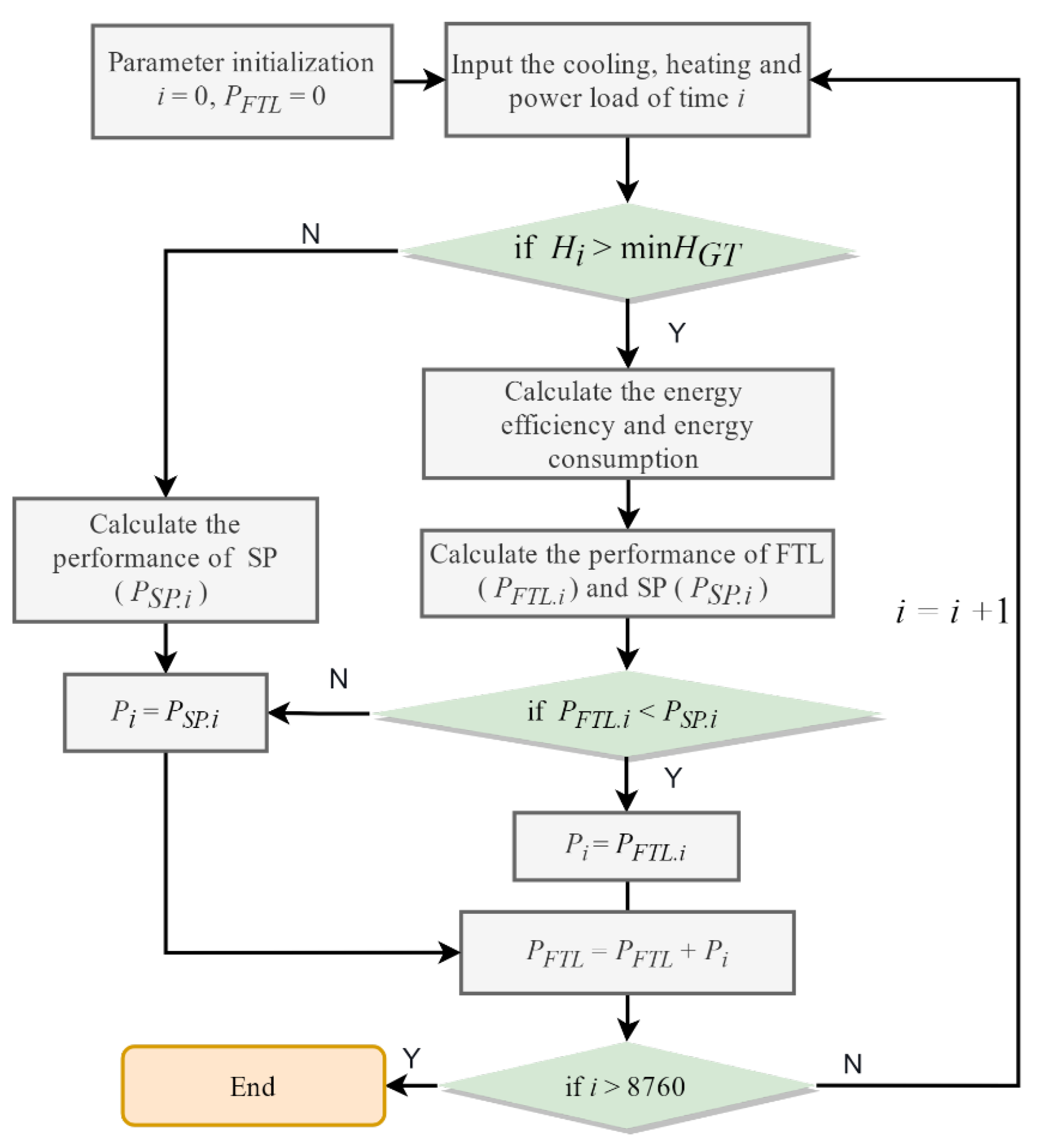
2.5.2. FTL Operational Strategy

The operating principle of FTL is similar to that of FEL. The difference between FEL and FTL is that when performing FTL, the load rate of the gas turbine is determined by the building’s cooling and heating load. Under FTL, the operating efficiency of the gas turbine is determined by the thermal load of the building. If the power load demand is greater than the power generated by the DES, the municipal power grid supplements the deficit heat. Figure 5 shows the operational cost calculation process of the DES when performing FTL. The operational constraints of FEL are as follows:

$$x_i=\left\{\begin{array}{c}0 H_i<min{H}_{gt} \hfill \\ \frac{H_i}{V_{gt.H}} min{H}_{gt}\le H_i<V_{gt.H} \hfill \\ 1 V_{gt.H}\le H_i \end{array}\right.$$

(24)

$$H_{gb.i}^{ }=H_i-H_{gt.i}·{\eta }_{he}\ge 0$$

(25)

$$C_{er.i}^{ }=C_i-H_{gt.i}·{\eta }_{ar}\ge 0$$

(26)

$$E_{gb.i}^{ }=E_i-E_{gt.i}\ge 0$$

(27)

2.5.3. HOS Operational Strategy

To solve the problem of insufficient utilization of energy in the above operational strategies and to reduce the carbon dioxide emissions of the DES, HOS is proposed to comprehensively consider the structure of the load and the operating efficiency of the equipment. The cooling/electricity and heating/electricity ratio of the gas turbine and load at time i are as follows:

$$CE{R}_{gt}=H_{gt.i}^{ }·{\eta }_{ar}/E_{gt.i}^{ }$$

(28)

$$CE{R}_i=C_i/E_i$$

(29)

$$HE{R}_{gt}=H_{gt.i}^{ }/E_{gt.i}^{ }$$

(30)

$$HE{R}_i=H_i/E_i$$

(31)

As shown in Figure 6a, the operational mode of HOS in the summer is as follows:

(1)

CER_gt > CER_i and C_i > V_gt.H·η_ar

Under these circumstances, the cooling and power load demands are greater than the refrigerating output generated by the gas turbine and absorption refrigeration unit. The gas turbine operates at full load (x_i = 1) due to the load of the building being greater than the rated capacity of the gas turbine. The deficit cooling and power load are provided by the electric refrigerating unit and the municipal power grid.

(2)

CER_gt < CER_i and C_i < V_gt.H·η_ar

The cooling load of the building is lower than the rated refrigerating output of the absorption refrigeration unit. At this time, the cooling/electricity ratio of the building is higher than the equipment. The cooling load determines the load rate of the gas turbine, which does not waste energy. Therefore, performing FTL in this hour is the most reasonable solution under these circumstances.

(3)

CER_gt > CER_i and E_i·η_er + C_i > V_gt.E·η_er + V_gt.H·η_ar

The cooling/electricity ratio of the building is higher than the equipment and the total power of the gas turbine is lower than the building’s load demand. The rated capacity of the gas turbine may be greater than the power load demand of the building and the excess power generation can be provided to the electric refrigeration unit. Otherwise, the deficit power and cooling load is provided by the municipal power grid.

(4)

CER_gt < CER_i and E_i·η_er + C_i < V_gt.E·η_er + V_gt.H·η_ar

The rated capacity of the gas turbine is greater than the cooling load demand of the building. The power load of the building and the power consumption of the electric refrigeration unit can be met by the gas turbine. It was found that when the load rate of the gas turbine is equal to (E_i·η_er + C_i) E_{gt. i}/H_gt.i·η_ar, the gas turbine can exactly meet the cooling and power load of users. Under this operational mode, the efficiency of natural gas is maximum.

As shown in Figure 6b, the operational mode of HOS in the winter is as follows:

(1)

HER_gt > HER_i and H_i > V_gt.H

The operational model is similar to that in summer under these circumstances. The gas turbine operates at full load (x_i = 1). The difference is that the deficit heating and power load are provided by the gas-fired boiler and the municipal power grid.

(2)

HER_gt > HER_i and H_i < V_gt.H

The heating/electricity ratio of the building at time i is less than the gas turbine, and the heating load of the building is lower than the rated heating capacity of the gas turbine. The heating load determines the load rate of the gas turbine, which does not waste energy. Therefore, performing FTL in this hour is the most reasonable solution under these circumstances.

(3)

HER_gt < HER_i

The heating/electricity ratio of the building at time i is larger than the gas turbine. The electric load determines the load rate of the gas turbine, which does not waste energy. When the heat load demand of the building is less than the rated heating capacity of the gas turbine, performing FEL in this hour is the most reasonable solution. Otherwise, the gas turbine operates at full load (x_i = 1) and the deficit heat load demand is provided by gas-fired boilers.

2.6. Evaluating Indicator

To analyze the relationship between the optimization results of the DES and load fluctuation throughout the year, this study took annual total cost, carbon emissions, and energy efficiency as the evaluation indicators, as compared with SP. The annual total cost, carbon dioxide emissions, and energy efficiency were used as the evaluation indices. The equations are as follows.

$$AT{C}_{ }^{ }={\displaystyle \sum }_{i=1}^n\left(P_{E.i}·E_{U.i}^{ }+P_{gas}^{ }·G_{gt.i}^{ }+P_{gas}^{ }·G_{gb.i}^{ }\right)+{{\displaystyle \sum }}_{j=1}^{k}P{E}_j·V_j$$

(32)

$$C{E}_{ }^{ }={\displaystyle \sum }_{i=1}^n\left(E_i^{ }·{\delta }_E^{ }+G_i^{ }·{\delta }_{gas}^{ }\right)$$

(33)

$$E{E}_{ }^{ }=\frac{{{\displaystyle \sum }}_{i=1}^n\left(E_i^{ }+C_i+H_i\right)}{{{\displaystyle \sum }}_{i=1}^n\left(E_{U.i}^{ }·{\omega }_E+G_{gt.i}^{ }·Q_{gas}+G_{gb.i}·Q_{gas}\right)}$$

(34)

where P_E and P_gas are the pieces of electricity and natural gas, respectively; PE is the equipment cost of one kilowatt; k is the equipment quantity of the DES; Q_gas is the calorific value of natural gas; δ_E and δ_gas are the unit carbon emissions of consuming electricity and natural gas, respectively; and ω_E is the reciprocal of power generation efficiency of the power plant.

3. Case Study

The DES can be applied to many types of buildings. This study took an office building in Nanjing as an example with which to analyze the impact of the operational strategy and load fluctuation on DES operation and the optimization results.

3.1. Model Parameter

The optimization algorithm in this paper takes the highest comprehensive performance as the objective function. The price and calorific value of natural gas are 2.5 yuan/m³ and 36,000 kJ/m³, respectively. The electricity prices at different periods are shown in

Table 1. Electricity prices in different periods.

	Time	Price (Yuan·(kWh)−1)
Peak period	8:00~11:00 18:00~21:00	1.074
Intermediate period	6:00~8:00 11:00~18:00 21:00~22:00	0.671
Valley period	0:00~6:00 22:00~24:00	0.316

. The equipment parameters of the DES are shown in

Table 2. Cost, maintenance cost, operational efficiency, and life of main equipment.

Equipment	Equipment Cost (Yuan·(kWh)−1)	Maintenance Cost (Yuan·(kWh)−1)	Efficiency	Life (Year)
GT	6500	0.0472	${\eta }_{gt.E}$ *	30
			${\eta }_{gt.H}$ **
HRSG	800	0.0022	0.85	20
GB	900	0.0022	0.90	20
ER	900	0.0087	4.5	20
ARU	1228	0.008	1.2	20
HE	100	0	0.95	20

* The values of σ₁, σ ₂, σ _3, and σ ₄ are −1.8 × 10⁻⁸, 4.97 × 10⁻⁶, 4.99 × 10⁻⁵, 0.022 and 0.017, respectively [35]. ** The values of τ ₁, τ ₂, τ _3, and τ ₄ are −2.37 × 10⁻⁸, 6.41 × 10⁻⁶, 6.87 × 10⁻⁵, 0.028 and 0.022, respectively [35].

. It is assumed that the conversion coefficient of standard coal for the power generation of the power plant is 0.33 kg/kWh [36]. The carbon emission by natural gas combustion is 1.88 kg/m³ [37].

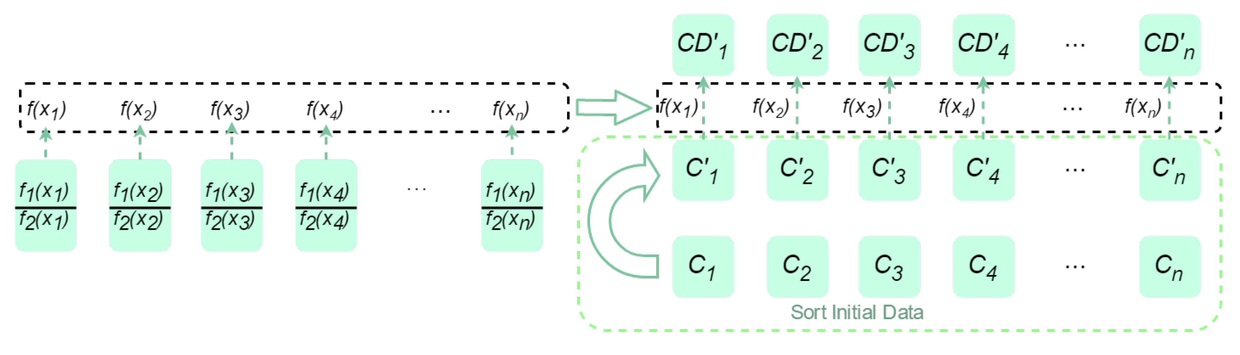
3.2. Load Discretization

The initial load of the building was obtained through DeST based on the building parameters. Thereafter, MATLAB was used to disperse the initial load to obtain the discrete load. Figure 7 and Figure 8 show the delayed load and the typical daily load of the discrete load with θ from −0.05 to 0.1. It was found that discretization changes the fluctuation of the annual load under the premise of the same total load. In addition, 100 sets of discrete loads with θ from −0.06 to 0.11 were obtained to avoid errors in the optimization results caused by the small sample size.

3.3. Optimization Results

After running the program 20 times, the deviation in the optimization result was less than 0.5% of the iterations, which met the calculation requirements. The optimization results of the evaluation index and equipment capacity under the three operational strategies are shown in

Table 3. The evaluation index optimization results of three operational strategies.

Operational Strategy	CEI	ATC (Yuan)	CE (t)	EE
HOS	0.151	3.22 × 106	3854	0.83
FEL	0.103	3.39 × 106	4056	0.79
FTL	0.076	3.42 × 106	4112	0.77

and

Table 4. The equipment capacity optimization results of three operational strategies.

Operational Strategy	GT (kW)	ER (kW)	GB (kW)	HRSG (kW)	ARU (kW)	HE (kW)
HOS	643	1334	2159	1922	2189	1762
FEL	704	1112	1865	2154	2320	1966
FTL	603	1224	2112	1789	1974	1523

. The CEI of HOS was 0.05 to 0.07 higher than those of FEL and FTL. The annual total cost and carbon dioxide emissions of HOS were lower than those of FEL and FTL. The energy efficiency of the DES-HOS was more than 0.8 higher than those of FEL and FTL. The reason for this was that the DES using HOS operates according to the most reasonable energy scheme for different load characteristics. As shown in Table 4, the equipment capacity of the DES-HOS was not the highest or lowest, proving that the optimal equipment configuration of the DES is based on a reasonable operational strategy.

In addition, in order to intuitively compare the operational efficiency of the DES under different operational strategies, the process of energy flow with different operational strategies in the optimization process was recorded, which included the conversion of energy among multiple devices and the loss in the process of operation of the DES. A Sankey diagram of energy flow is shown in Figure 9. It can be observed from the Sankey diagram of energy flow that the energy demand for grid power and natural gas was 9717 kW, which is about 13.2% less than those of FEL and FTL when HOS was implemented. Moreover, the energy waste of the DES-HOS was 1879 kW, which was 19.7% and 15.5% lower than those of FEL and FTL, respectively. Therefore, it was found that the HOS can reduce the energy consumption and waste of the DES under the same building load.

The 100 sets of discrete loads with a θ from −0.06 to 0.11 and their typical daily loads were input into the algorithm for the optimization of the DES-HOS. The scatters and fitting lines of the ATC, CE, EE, and CEI are shown in Figure 10. The annual total cost of the DES optimized based on annual hourly load was 4.7% to 6.2% less than that of a typical daily load (Figure 10a). The annual operational cost of the DES-HOS increased by 3.4% and 6.5% as the θ increased from −0.05 to 0.1, respectively. The increase in grid power consumption was the main reason for the increase in the annual operational cost of the DES-HOS. Figure 10b shows that the carbon emissions of the DES optimized base on annual hourly load were 8.7% to 12.5% less than the typical daily load. The energy efficiency of the DES optimized base on annual hourly load was 2.5% to 4.7% higher than the typical daily load (Figure 10c). As θ increased from −0.05 to 0.1, the energy efficiency of the DES decreased by 2.1% and 5.3%, respectively. Figure 10d shows that the CEI of the DES-HOS based on annual hourly load was 4.7% to 6.2% less than the typical daily load. As the θ increased from −0.05 to 0.1, the CEI of the DES-HOS decreased by 1.8% to 2.6%, respectively.

The reasons for the above differences are related to the capacity configuration of the DES-HOS and the input of energy.

Table 5. The equipment capacity of the DES-HOS with a θ from −0.05 to 0.1.

θ	GT (kW)	ER (kW)	GB (kW)	HRSG (kW)	ARU (kW)	HE (kW)
−0.05	723	1121	1974	2120	2354	1862
0	643	1334	2159	1922	2189	1762
0.05	594	1485	2310	1781	1910	1642
0.1	550	1610	2521	1665	1759	1519

and

Table 6. The input and waste energy of the DES-HOS with a θ from −0.05 to 0.1.

θ	Gas (×105 m3)	Power * (MWh)	Waste (MWh)
−0.05	6.94	3021	1811
0	6.74	2993	1924
0.05	6.51	3710	2045
0.1	6.22	4156	2141

* Power supply from the power grid.

show the equipment capacity and the input and waste energy of the DES-HOS optimization results with a θ of −0.05, 0, 0.05, and 0.1. Table 5 shows that with the increase in θ, the rated capacity of the gas turbine decreased from 723 kW to 550 kW, which means that the compatibility between the DES-HOS and the building load became worse. Table 6 shows that with the increase in θ, the input of gas decreased from 6.94 × 10⁵ m³ to 6.22 × 10⁵ m³ and the input of power decreased from 3021 MWh to 4156 MWh. With the increase in θ, the waste energy of the DES-HOS increased from 1811 MWh to 2141 MWh. Moreover, the change in the equipment capacity and energy consumption structure of the DES-HOS led to an increase in carbon dioxide emissions.

4. Conclusions

This paper incorporates the hybrid operational strategy into the multi-objective optimization model to optimize the equipment capacity of a DES. An office building was taken as an example with which to compare and analyze the comprehensive performance of the DES under different operational strategies and load structures. The conclusions are as follows:

(1)

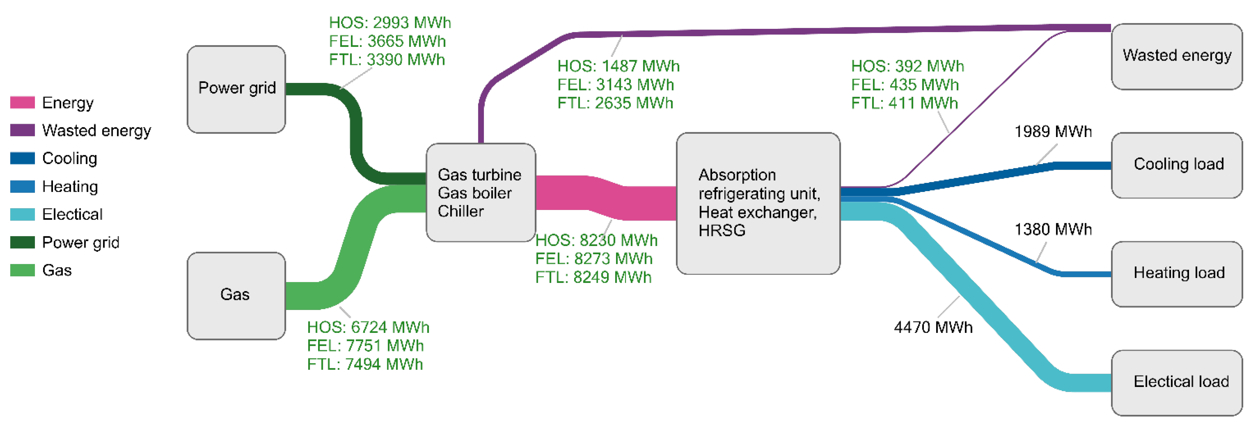
Compared with the FEL and FTL operational strategies, the HOS reduced the energy waste of the DES by 19.7% and 15.5% and improved the comprehensive performance of the DES by 5.2% and 7.1%, respectively, through the cooperation between the annual hourly load characteristics and the equipment efficiency.

(2)

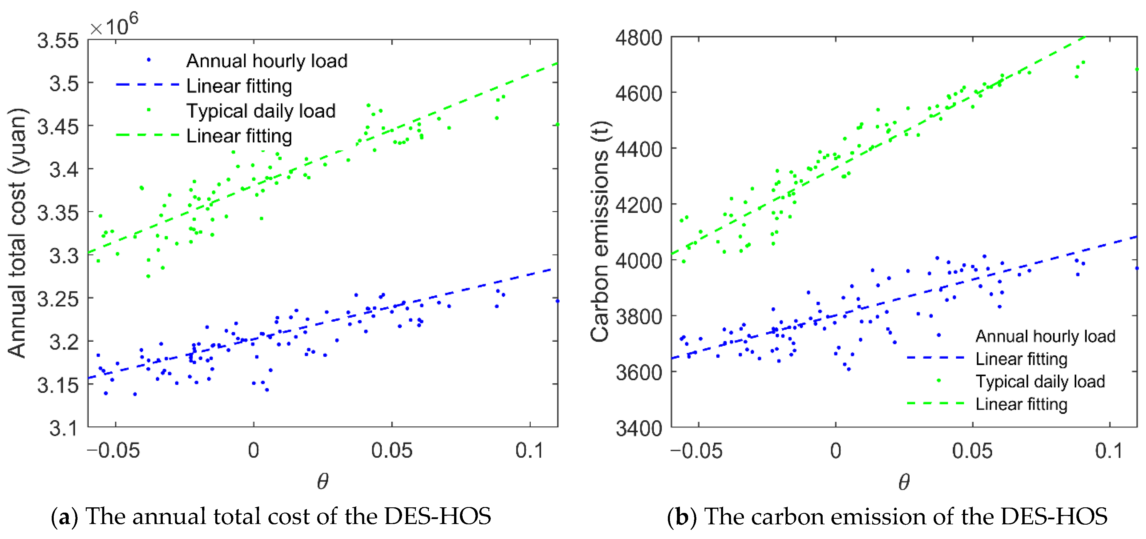
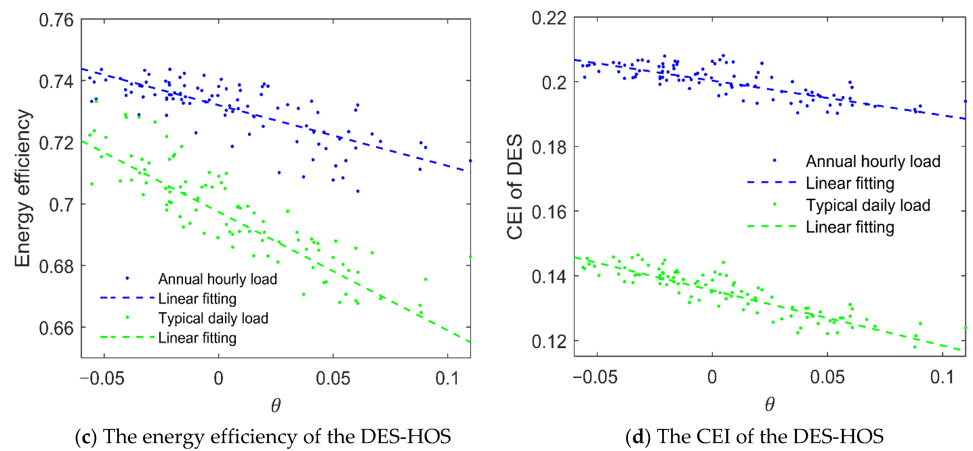
According to the performance analysis of the DES optimized based on multiple sets of discrete load with different fluctuations, it was found that the comprehensive performance of the DES-HOS decreased by 1.8% with the increase in the load fluctuation by 15%.

(3)

Compared with using a typical daily load, using the annual hourly load for DES-HOS optimization improved the accuracy of load forecasting and the comprehensive performance of the DES by about 5.2% and lowered the adverse impact derived from load fluctuations.

References

1. Ren, F.; Wei, Z.; Zhai, X. A review on the integration and optimization of distributed energy systems. Renew. Sustain. Energy Rev. 2022, 162, 112440. [Google Scholar] [CrossRef]
2. Vaccari, M.; Mancuso, G.; Riccardi, J.; Cantù, M.; Pannocchia, G. A Sequential Linear Programming algorithm for economic optimization of Hybrid Renewable Energy Systems. J. Process Control 2017, 2017 74, 189–201. [Google Scholar] [CrossRef]
3. Mago, P.J.; Fumo, N.; Chamra, L.M. Performance analysis of CCHP and CHP systems operating following the thermal and electric load. Int. J. Energy Res. 2010, 33, 852–864. [Google Scholar] [CrossRef]
4. Wang, J.; Dong, F.; Ma, Z.; Chen, H.; Yan, R. Multi-objective optimization with thermodynamic analysis of an integrated energy system based on biomass and solar energies. J. Clean. Prod. 2021, 324, 129257. [Google Scholar] [CrossRef]
5. Li, M.; Zhou, M.; Feng, Y.; Mu, H.; Ma, Q.; Ma, B. Integrated design and optimization of natural gas distributed energy system for regional building complex. Energy Build. 2017, 154, 81–95. [Google Scholar] [CrossRef]
6. Ge, Y.; Han, J.; Ma, Q.; Feng, J. Optimal configuration and operation analysis of solar-assisted natural gas distributed energy system with energy storage. Energy 2022, 246, 123429. [Google Scholar] [CrossRef]
7. de Doile, G.N.; Junior, P.R.; Rocha, L.C.; Janda, K.; Aquila, G.; Peruchi, R.S.; Balestrassi, P.P. Feasibility of Hybrid Wind and Photovoltaic Distributed Generation and Battery Energy Storage Systems Under Techno-Economic Regulation. Renew. Energy 2022, 195, 1310–1323. [Google Scholar] [CrossRef]
8. Liu, Z.; Guo, J.; Wu, D.; Fan, G.; Zhang, S.; Yang, X.; Ge, H. Two-phase collaborative optimization and operation strategy for a new distributed energy system that combines multi-energy storage for a nearly zero energy community. Energy Convers. Manag. 2021, 230, 113800. [Google Scholar] [CrossRef]
9. Liu, Z.; Li, Y.; Fan, G.; Wu, D.; Guo, J.; Jin, G.; Zhang, S.; Yang, X. Co-optimization of a novel distributed energy system integrated with hybrid energy storage in different nearly zero energy community scenarios. Energy 2022, 247, 123553. [Google Scholar] [CrossRef]
10. Wen, Q.; Liu, G.; Rao, Z.; Liao, S. Applications, evaluations and supportive strategies of distributed energy systems: A review. Energy Build. 2020, 225, 110314. [Google Scholar] [CrossRef]
11. Jan, J.; Broesicke, O.; Tong, X.; Wang, D.; Li, D.; Crittenden, J.C. Multidisciplinary design optimization of distributed energy generation systems: The trade-offs between life cycle environmental and economic impacts. Appl. Energy 2020, 284, 116197. [Google Scholar]
12. Ma, W.; Fang, S.; Liu, G. Hybrid optimization method and seasonal operation strategy for distributed energy system integrating CCHP, photovoltaic and ground source heat pump. Energy 2017, 141, 1439–1455. [Google Scholar] [CrossRef]
13. Gou, X.; Chen, Q.; Sun, Y.; Ma, H.; Li, B.-J. Holistic analysis and optimization of distributed energy system considering different transport characteristics of multi-energy and component efficiency variation. Energy 2021, 228, 120586. [Google Scholar] [CrossRef]
14. Vaccari, M.; di Capaci, R.B.; Brunazzi, E.; Tognotti, L.; Pierno, P.; Vagheggi, R.; Pannocchia, G. Optimally Managing Chemical Plant Operations: An Example Oriented by Industry 4.0 Paradigms. Ind. Eng. Chem. Res. 2021, 60, 7853–7867. [Google Scholar] [CrossRef]
15. Liu, Z.; Guo, J.; Li, Y.; Wu, D.; Zhang, S.; Yang, X.; Ge, H.; Cai, Z. Multi-scenario analysis and collaborative optimization of a novel distributed energy system coupled with hybrid energy storage for a nearly zero-energy community. J. Energy Storage 2021, 41, 102992. [Google Scholar] [CrossRef]
16. Huang, D.; Zhou, D.; Jia, X.; Yan, S.; Li, T.; Huang, D.; Zhang, C. A mixed integer optimization method with double penalties for the complete consumption of renewable energy in distributed energy systems. Sustain. Energy Technol. Assess. 2022, 52, 102061. [Google Scholar] [CrossRef]
17. Guo, J.; Zhang, P.; Wu, D.; Liu, Z.; Ge, H.; Zhang, S.; Yang, X. A new collaborative optimization method for a distributed energy system combining hybrid energy storage. Sustain. Cities Soc. 2021, 75, 103330. [Google Scholar] [CrossRef]
18. Huang, Y.; Xu, P.; Wu, Q.; Ren, H.; Li, Q.; Yang, Y. Optimization of regional distributed energy system under discrete demand distribution. Energy Rep. 2022, 8, 634–640. [Google Scholar] [CrossRef]
19. Li, L.; Mu, H.; Li, N.; Li, M. Analysis of the integrated performance and redundant energy of CCHP systems under different operation strategies. Energy Build. 2015, 99, 231–242. [Google Scholar] [CrossRef]
20. Wu, J.-Y.; Wang, J.-L.; Li, S. Multi-objective optimal operation strategy study of micro-CCHP system. Energy 2012, 48, 472–483. [Google Scholar] [CrossRef]
21. Zhou, Y.; Wang, J.; Dong, F.; Qin, Y.; Ma, Z.; Ma, Y.; Li, J. Novel flexibility evaluation of hybrid combined cooling, heating and power system with an improved operation strategy. Appl. Energy 2021, 300, 117358. [Google Scholar] [CrossRef]
22. Peng, X.; Bhattacharya, T.; Cao, T.; Mao, J.; Tekreeti, T.; Qin, X. Exploiting Renewable Energy and UPS Systems to Reduce Power Consumption in Data Centers. Big Data Res. 2021, 27, 100306. [Google Scholar] [CrossRef]
23. Wang, Y.; Zou, C.; Li, W.; Zou, Y.; Huang, H. Improving stability and thermal properties of TiO2 nanofluids by supramolecular modification: High energy efficiency heat transfer medium for data center cooling system. Int. J. Heat Mass Transf. 2020, 156, 119735. [Google Scholar] [CrossRef]
24. Cao, Y.; Wu, Y.; Fu, L.; Jermsittiparsert, K.; Razmjooy, N. Multi-objective optimization of a PEMFC based CCHP system by meta-heuristics. Energy Rep. 2019, 5, 1551–1559. [Google Scholar] [CrossRef]
25. Mu, Y.; Wang, C.; Sun, M.; He, W.; Wei, W. CVaR-based operation optimization method of community integrated energy system considering the uncertainty of integrated demand response. Energy Rep. 2022, 8, 1216–1223. [Google Scholar] [CrossRef]
26. Rajamand, S. Probabilistic Power Distribution Considering Power Uncertainty of Load and Distributed Generators Using Cumulant and Truncated Versatile Distribution. Sustain. Energy Grids Netw. 2022, 30, 100608. [Google Scholar] [CrossRef]
27. Li, L.; Cao, X.; Wang, P. Optimal coordination strategy for multiple distributed energy systems considering supply, demand, and price uncertainties. Energy 2021, 227, 120460. [Google Scholar] [CrossRef]
28. Lu, C.; Wang, J.; Yan, R. Multi-objective optimization of combined cooling, heating and power system considering the collaboration of thermal energy storage with load uncertainties. J. Energy Storage 2021, 40, 102819. [Google Scholar] [CrossRef]
29. Liu, Z.; Cui, Y.; Wang, J.; Yue, C.; Agbodjan, Y.S.; Yang, Y. Multi-objective optimization of multi-energy complementary integrated energy systems considering load prediction and renewable energy production uncertainties. Energy 2022, 254, 124399. [Google Scholar] [CrossRef]
30. Hou, J.; Wang, J.; Zhou, Y.; Lu, X. Distributed energy systems: Multi-objective optimization and evaluation under different operational strategies. J. Clean. Prod. 2020, 280, 124050. [Google Scholar] [CrossRef]
31. Lee, D.; Kim, B.J. Different environmental conditions in genetic algorithm. Phys. A Stat. Mech. Its Appl. 2022, 602, 127604. [Google Scholar] [CrossRef]
32. Zakaria, A.; Ismail, F.B.; Lipu, M.H.; Hannan, M. Uncertainty models for stochastic optimization in renewable energy applications. Renew. Energy 2020, 145, 1543–1571. [Google Scholar] [CrossRef]
33. Rojas, C.; Troubetzkoy, S. Coding discretizations of continuous functions. Discret. Math. 2011, 311, 620–627. [Google Scholar] [CrossRef]
34. Lai, J.Z.; Huang, T.-J. An agglomerative clustering algorithm using a dynamic k-nearest-neighbor list. Inf. Sci. 2011, 181, 1722–1734. [Google Scholar] [CrossRef]
35. Gou, X.; Zhang, H.; Li, G.; Cao, Y.; Zhang, Q. Dynamic simulation of a gas turbine for heat recovery at varying load and environment conditions. Appl. Therm. Eng. 2021, 195, 117014. [Google Scholar] [CrossRef]
36. Momeni, M.; Soltani, M.; Hosseinpour, M.; Nathwani, J. A comprehensive analysis of a power-to-gas energy storage unit utilizing captured carbon dioxide as a raw material in a large-scale power plant. Energy Convers. Manag. 2021, 227, 113613. [Google Scholar] [CrossRef]
37. Azam, A.; Rafiq, M.; Shafique, M.; Zhang, H.; Yuan, J. Analyzing the effect of natural gas, nuclear energy and renewable energy on GDP and carbon emissions: A multi-variate panel data analysis. Energy 2021, 219, 119592. [Google Scholar] [CrossRef]
Figure 1. The typical structure of the DES and SP.
Applsci 12 09449 g001
Figure 2. The flow chart of the optimization model.
Applsci 12 09449 g002
Figure 3. The process of discretization for the initial cooling load.
Applsci 12 09449 g003
Figure 4. Flowchart of FEL operational strategy.
Applsci 12 09449 g004
Figure 5. Flowchart of FTL operational strategy.
Applsci 12 09449 g005
Figure 6. Flowchart of HOS operational strategy in the summer (a) and winter (b).
Applsci 12 09449 g006
Figure 7. Delayed load curve of power load (a), and cooling and heating load (b) at the θ of –0.05, 0, 0.05, and 0.1.
Applsci 12 09449 g007
Figure 8. Typical daily load of the power load in the summer (a) and in the winter (b) at the θ of –0.05, 0, 0.05, and 0.1.
Applsci 12 09449 g008
Figure 9. The energy flow of the DES with HOS, FEL and ETL.
Applsci 12 09449 g009
Figure 10. Variations of the DES-HOS annual total cost (a), carbon emission (b), energy efficiency (c) and CEI (d) with the rise in load fluctuation.
Applsci 12 09449 g010aApplsci 12 09449 g010b