Abstract
A downhole electric tubular resistive heater is proposed for the oil-shale in situ resorting. After flowing through a set of heating tubes, the outlet temperature and the flow rate of the injected gas can be conveniently adjusted to match the requirement of the pyrolysis temperature of the oil shale. The calculation demonstrates the effects of the inner diameter, the length of the heating tube, and the inlet flow rate on the heat transfer performance of the electric heater. It was found that, compared with the armored electric heaters, even with a small inject flow rate of 5 Nm3/min, the convective heat transfer coefficient of the inner flow exceeds 300 W/m2 K, resulting in a much smaller thermal resistance. The outlet temperature of the heating gas can conveniently reach up to 900 °C with the absence of the complex structure of enhanced fins. Though the pressure loss is relatively larger under a high flow rate, the comprehensive index is still 40% higher, indicating that the present tubular electric heater is a promising candidate to deal with complex downhole conditions.
1. Introduction
Oil shale is a lamellar and impermeable sedimentary rock, which contains large amounts of kerogen that can be decomposed into smaller molecules to produce oil, gas, and carbonaceous coke by pyrolysis or retorting [1]. The development of oil-shale resources has attracted increasing interest due to the tremendous increase in global energy demand and rapid depletion of conventional oil resources [2].
Traditionally, the shale oil is produced aboveground by mining the oil shale and then post-treating it in proceeding facilities [3]. However, opencast mining occupies much land and produces a large amount of polluted gas, acidic water, and waste residues. In the past few decades, the in situ resorting technologies for the production of hydrocarbons from oil shale have been developed significantly, including conductive heating [4], convective heating [5], combustion [6], and the radiant heating [7]. Among these technologies, the downhole electric resistive heaters are still believed to be the optimal method for oil-shale in situ resorting, as they have been widely used in the exploitation of shale oil in various fields.
Shell developed the in situ conversion process for oil-shale exploitation [4] by heating the oil-shale deposit by using the electric resistive heaters. Due to the limited heat-transfer area, the heating conduction efficiency of the bare electric heater is pretty low, which takes over one year to heat the oil shale before mass production [8]. Thus, recent studies focus on expanding the heat-transfer area of the electric resistive heater by adding various kinds of enhanced fins [9,10,11,12,13,14,15,16]. Wang et al. [9] proposed a double-shell-structured downhole electric heater with continuous helical baffles, which improved the heating efficiency of the downhole electric heaters effectively. Later, Gu et al. [10] claimed that the electric heater with the axial separation helical baffle schemes showed better comprehensive index and temperature uniformity than those of the segment baffle ones. Guo et al. [11] also found that the heater with continuous helical baffles was more suitable for downhole heating than that with segmental baffles in terms of the long-term working stability by simulation and experiments. Yang et al. [12] studied the downhole unilateral-ladder-type helical baffle heat exchangers with folded baffles and found that the shell-side heat-transfer coefficients were larger, but the comprehensive indexes were smaller than those of the corresponding plane ones. Wang et al. [13] proposed the trisection-helical-baffled electric heaters to overcome the defects in conventional segmental-baffled ones. Tang et al. [14] designed a novel configuration of the axial-separation helical-baffle heat exchangers and solved the problem in the seriation of the helical-baffle angles to reduce the fabrication cost.
All the electric resistive heaters with enhanced fins are mineral insulated to preserve and protect the purity and electrical properties of the core heating elements. Generally, the armored electric heaters are filled with high-quality electrical-grade magnesium oxide (MgO) powder due to its high dielectric and thermal conductivities. However, due to the rapid degradation of the electrical resistivity of MgO powder when the operating temperature is above 800 °C [17], the high nickel alloy sheath, MgO dielectric insulation, and resistance wire construction allow the tracing of heater temperature up to 600 °C for the armored electric heaters, much smaller than that of the bare electric heaters (~1000 °C). Note that the pyrolysis temperature of oil shale may range from 350 °C to 560 °C [18]. The lower operating temperature of the armored electric heaters requires complex fin structures to expand the heat transfer area. Accounting for the heavy weight and poor rigidity, special attention should be paid to the transportation and installation of the spiral plated heat exchangers, especially under the complex downhole conditions.
2. Design and Simulations
In this section, the downhole electric heater is designed. The fluid domain is extracted from the 3D configuration. The details on the governing equations and implementation of the standard k-ε turbulence model is described. The numerical method and boundary conditions are explained. Finally, a grid independence study is performed to ensure the validity of the numerical analysis.
2.1. Electric Tubular Heater Design
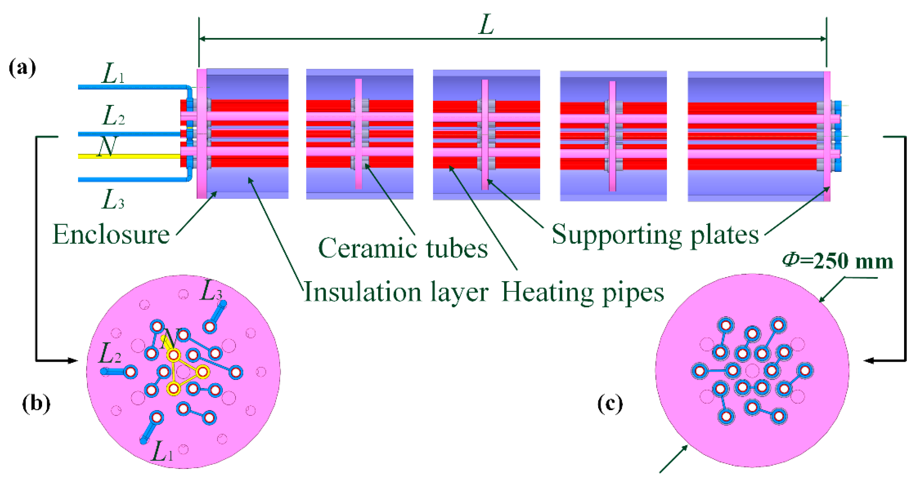
The designed tubular heater is adaptable to be run in inclined wells for oil-shale in situ resorting. The geometric model of the novel electric downhole tubular heater is presented in Figure 1a. The electric heater mainly consists of the following parts: (1) power cables (L1, L2, L3, and N) for delivering the electrical energy; (2) heating tubes for heating the gas flow to achieve the pyrolysis temperature of the oil shale; (3) an enclosure for withstanding the downhole operation pressure; (4) an insulation layer to reduce the heat loss and to avoid the creep deformation of the enclosure [19]; (5) supporting plates, which are used to align the tubular heaters to prevent the short circuit; and (6) ceramic tubes, which are used to insulate the support plates from the tubular heaters. Figure 1b,c present the left (inlet part of the flow) and right (outlet part of the flow) cross-sectional views of the layout of heating tubes. The tubular heaters are arranged in a three-phase electricity system. In each phase, the heating current passes through six tubular resistors that are connected in a series. The nitrogen gas with ambient temperature is fed into the heating tubes and flows from the left to right sides of the tube arrays. The thermal performance of the heater is evaluated by the numerical calculation of the temperature, velocity, and pressure fields. A control-variable scheme is applied by changing the heater geometrical parameters, such as tube lengths (L) and diameters (d), operating conditions (mass flow rate G), etc.
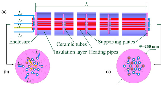
Figure 1.
Geometric model of electric heater: (a) front view of electric heater, (b) left view, and (c) right view of layout schemes of heating tubes.
In the initial thermal design, the outer dimeter of the tubular heater is set to 250 mm to fit the downhole well dimension. The upper limit of the tube length is 7 m to save the manufacturing cost. The thickness of the insulation layer is no less than 50 mm to ensure that more than 95% of the electric heating can be absorbed by the nitrogen gas. In the restricted space, the corresponding inner-tube diameter should be less than 8 mm.
2.2. Mathematical Models
The commercial Computational Fluid Dynamics (CFD) software (Ansys FLUENT 19.0) is adopted to perform the numerical simulations. In the simulation, the flow and heat transfer in the electric heater are governed by conversation, momentum, and energy-conversation equations. In view of the long heating pipe (>5 mm) with a small inner diameter (<10 mm), the entry region can be ignored. For the fully developed turbulent flow, the standard k-ε model is sufficient with reasonable accuracy, and the similar results are expected to be obtained from different turbulent models. The Semi-Implicit Method for Pressure Linked Equations (SIMPLE) algorithm is employed to address the coupling of velocity and pressure. For the fully developed turbulent region, the boundary-layer profile can be divided into the viscous sublayer, buffer layer, log-law region inner layer, and outer region. The sublayer region can be up to y+ < 10, and the log-law region is applied for y+ > 30. The buffer layer in between cannot be precisely resolved. In our calculation, the inner-tube diameter ranges from 5 mm to 7 mm. If there are 24 heating pipes, for the largest flow rate G = 10 Nm3/min, the nitrogen velocity is calculated to be smaller than 5 m/s with a downhole pressure of 10 Mpa and temperature of 50 °C, the corresponding Reynolds number is about 105. Considering the large Reynolds number, the turbulent boundary layer can be in a small impact on the flow velocity. Therefore, the standard wall functions are adopted. The benefit of the wall-function approach lies in a significant reduction in mesh resolution.
The governing equations for turbulence flow can be stated as follows [20]:
Continuity equation:
Momentum equation:
Energy equation for fluid flow:
Energy equation for solid:
where Pr is the Prandtl number, k is the turbulent kinetic energy, ui is the average velocity, ui′ is the fluctuating velocity, and T′ is the fluctuating temperature. The turbulent stress, , in Equation (2) and the turbulent heat flux, , in Equation (3) can be calculated as follows:
In the standard k-ε model, when the effects of buoyancy, as well as the flow compressibility (small March number) on the turbulence model are neglected, the turbulent kinetic energy, k, and its dissipation rate, ε, are described as follows:
Gk is the production of the turbulence kinetic energy, which is defined as follows:
In the simulation, the model constants are as follows: αk = 1.0, αε = 1.3, C1ε = 1.44, C2ε = 1.92, Cμ = 0.09, σk = 1.0, and σε = 1.3.
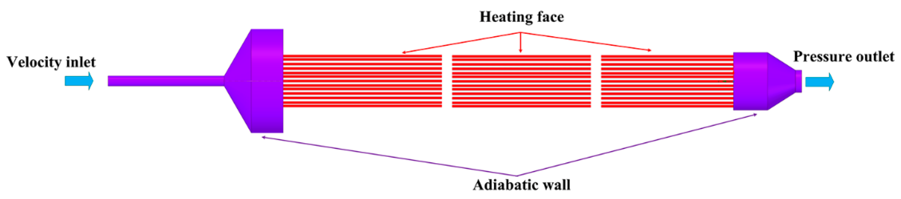
The nitrogen is considered to be incompressible, whose gravity is ignored. The material of the heating resistance is 20Cr80Ni. The boundary conditions are shown in Figure 2. The velocity inlet and pressure outlet are applied. The heating surfaces are set to be heating walls, where the surface heat flux is calculated from the heating power of the electric heater with a constant current of 100 A. The remaining walls are assumed to be adiabatic. The operation pressure is 10 MPa. Considering the temperature variation of the physical parameters of nitrogen, the polynomial fitting of the relevant physical parameters, including the density, thermal conductivity, viscosity, and specific heat, are applied, as shown in Table 1.

Figure 2.
Thermal boundary conditions of the electric heater.

Table 1.
The polynomial fitting of the thermophysical parameters of nitrogen versus temperature when the working pressure is 10 MPa. Here, the Kelvin temperature is adopted.
2.3. Data Reduction
The resistance per unit length of the heating tube can be calculated by
where ρe is the resistivity, and D and d are the outer and inner diameter of the heating pipe, respectively. The heating power of a single tube can be calculated by the following:
where L is the length of the single heating tube, and I is the working current. The heat transfer coefficient is as follows:
where Atotal is the total heat exchange area, Twall is the average temperature of the heating tube, and Tin and Tout are the inlet and outlet temperature, respectively. The pressure difference between the inlet and outlet of the electric heater can be expressed as follows:
2.4. Grid Independence Validation
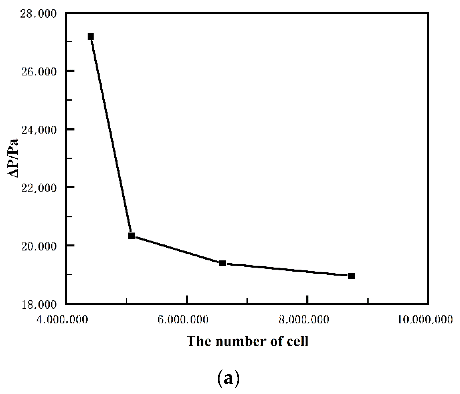
The geometry of the electric heater is created by the software CREO and pretreated by the software Ansys SCDM. The Ansys Fluent meshing mode is used to generate the unstructured poly mesh of the electric heater. The grid independence test is conducted with 4.4 M (million), 5.1 M, 6.6 M, and 8.7 M grids, as shown in Figure 3a. It is found that the growth rate of ΔP decreases with the increase of the grid number, and ΔP stabilizes when the grid number is 8.7 M. Considering the computational efficiency and precision, the final grid number is selected approximately 8.7 M. Fluent meshing provides an efficient and intelligent meshing solutions. Figure 3b shows the mesh grids of the inlet part of the electric heater.
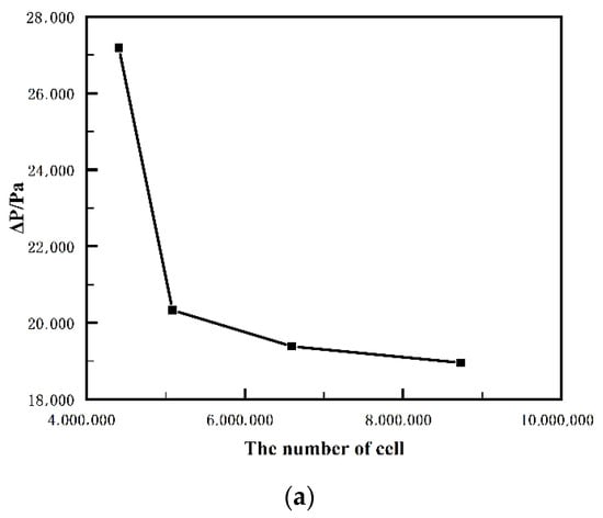

Figure 3.
Grids of electric heater: (a) grid independence validation and (b) meridian-section views of the inlet region.
3. Results and Discussion
In this section, the heat transfer and flow performance of the electric heater are analyzed based on the previous calculation setup. The effects of the structural parameters, including the inner diameter and length of the heating pipe, as well as the operation parameters, such as the inlet flow rate, are discussed. Finally, the heat transfer and flow performance are compared with the results from the downhole electric heater with continuous helical baffles under the same working condition.
3.1. Effect of Inner Diameter of Heating Tube
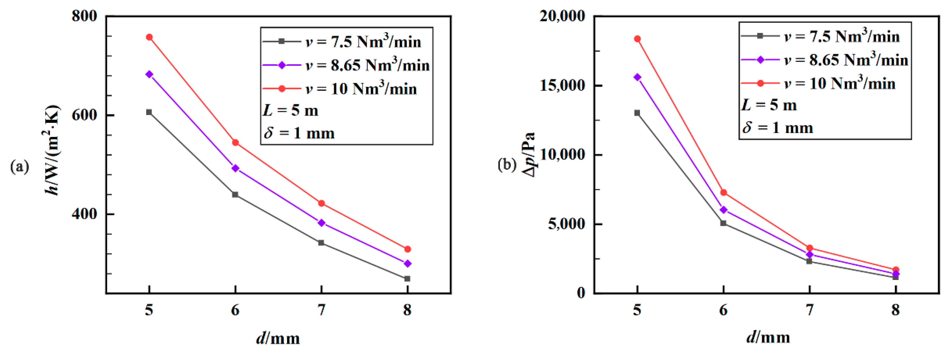
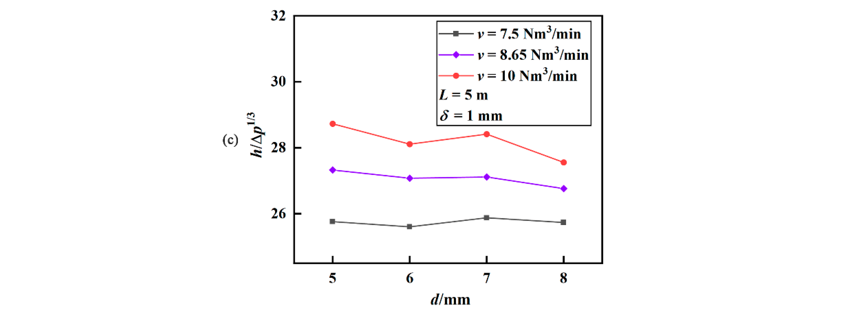
By changing the inlet flow rates and the inner diameters of the heating tube, the performance of the electric heater under different conditions is studied. The range of the inner diameter of the tube is 5–8 mm, and the range of the inlet mass flow rate is 7.5–10 Nm3/min. Figure 4a–c show the curves of the heat-transfer coefficient, pressure drop, and comprehensive index, h/Δp1/3, versus the inner diameter of the heating tube, respectively. It is found that a large inner diameter of the heating tube leads to the reduction of the heat-transfer coefficient and the pressure drop. As shown in Figure 4c, the comprehensive index, h/Δp1/3, changes non-monotonically within the range of 5–8 mm, showing a uniformly decline trend.
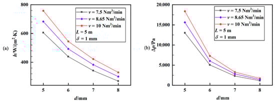

Figure 4.
Heat transfer and flow performance versus inner diameter of heating tube at different flow rates: (a) h, (b) Δp, and (c) h/Δp1/3.
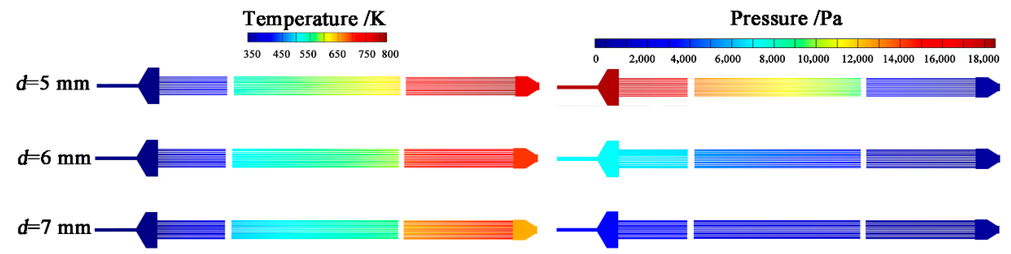
Figure 5 compares the temperature nephogram and pressure nephogram of the electric heater. From Equations (8) and (9), when the heating current is maintained the same, a large inner diameter gives rise to a small electrical resistance, resulting in a small heating power of a single tube. Therefore, the maximum temperature of the heating pipe with a smaller tube diameter is expected to be larger. Meanwhile, the small inner diameter of the heating-tube results in a large pressure loss along the tube, as shown in Figure 5. As a consequence, the relatively small tube is beneficial to the operations of the downhole electrical heater, whose convective heat transfer coefficient and comprehensive index are larger; meanwhile, the pressure loss (~18,500 Pa) and surface temperature of the heater (~850 °C) are still affordable.

Figure 5.
Temperature nephogram and pressure nephogram of electric heater at different inner diameters of heating pipes with flow rate G =10 Nm3/min, tube length L = 5 m, and tube thickness δ = 1 mm.
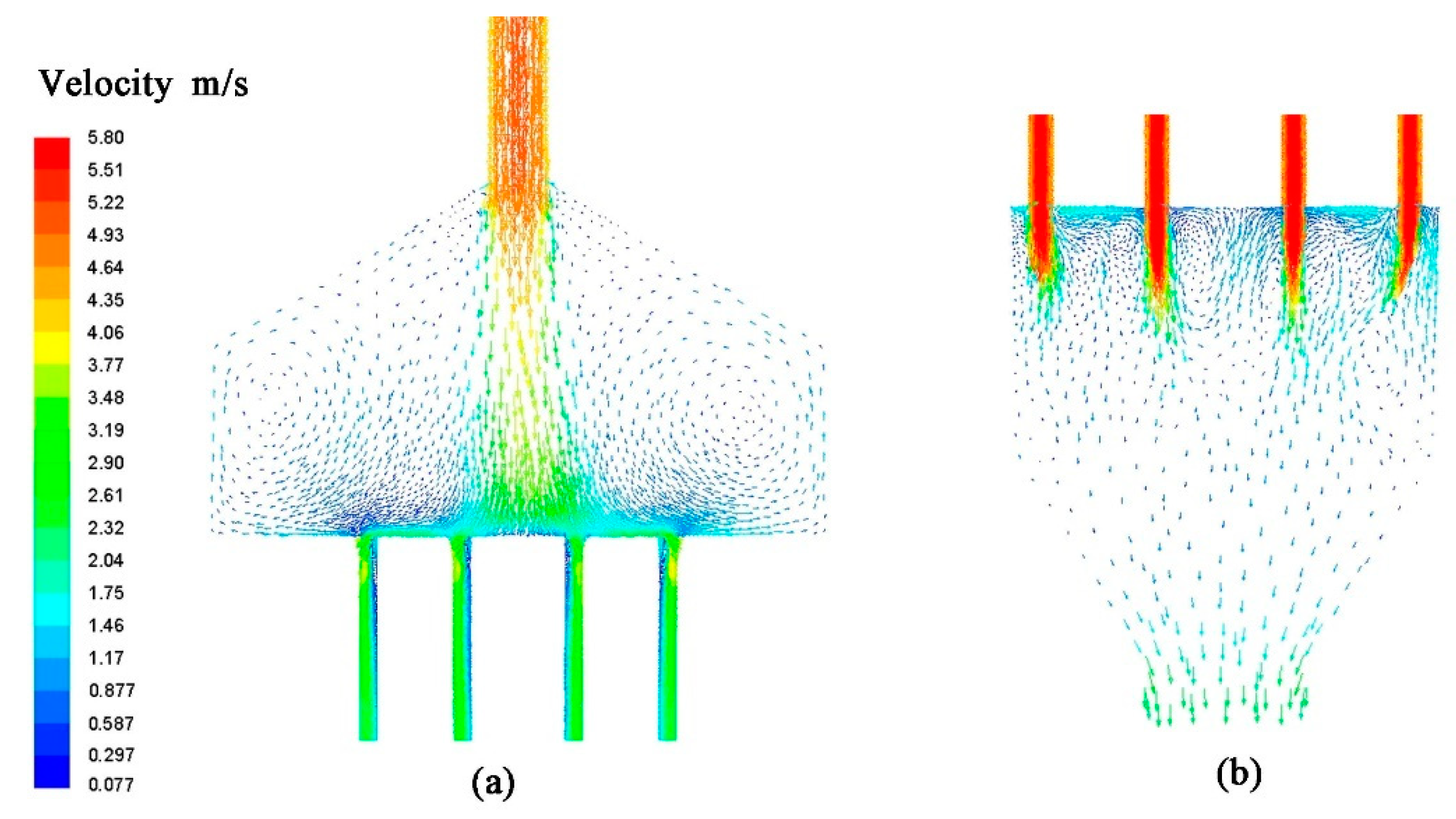
Figure 6 shows the typical velocity vectors in meridian slices. In the inlet chamber, the secondary vortex flows are formed, which ensures that the flow rates within the heating pipes are uniformly distributed. When nitrogen gas flows through a series of heating pipes, the velocity increases from about 2.8 m/s to about 6 m/s, due to the dramatic decrement in density as the temperature increases. When the high-speed nitrogen gas is injected into the outlet chamber, several small secondary vortex flows are formed, and the outlet velocity of the electric heater is estimated to be less than 1 m/s.
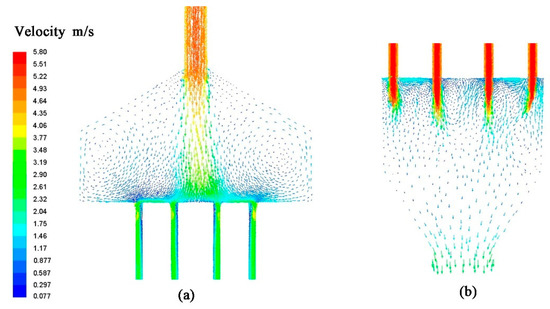
Figure 6.
Typical velocity vectors on meridian slices with flow rate G = 10 Nm3/min, tube length L = 5 m, tube length L = 5 m, and tube thickness δ = 1 mm: (a) inlet region and (b) outlet region.
3.2. Effect of Length of Heating Pipe
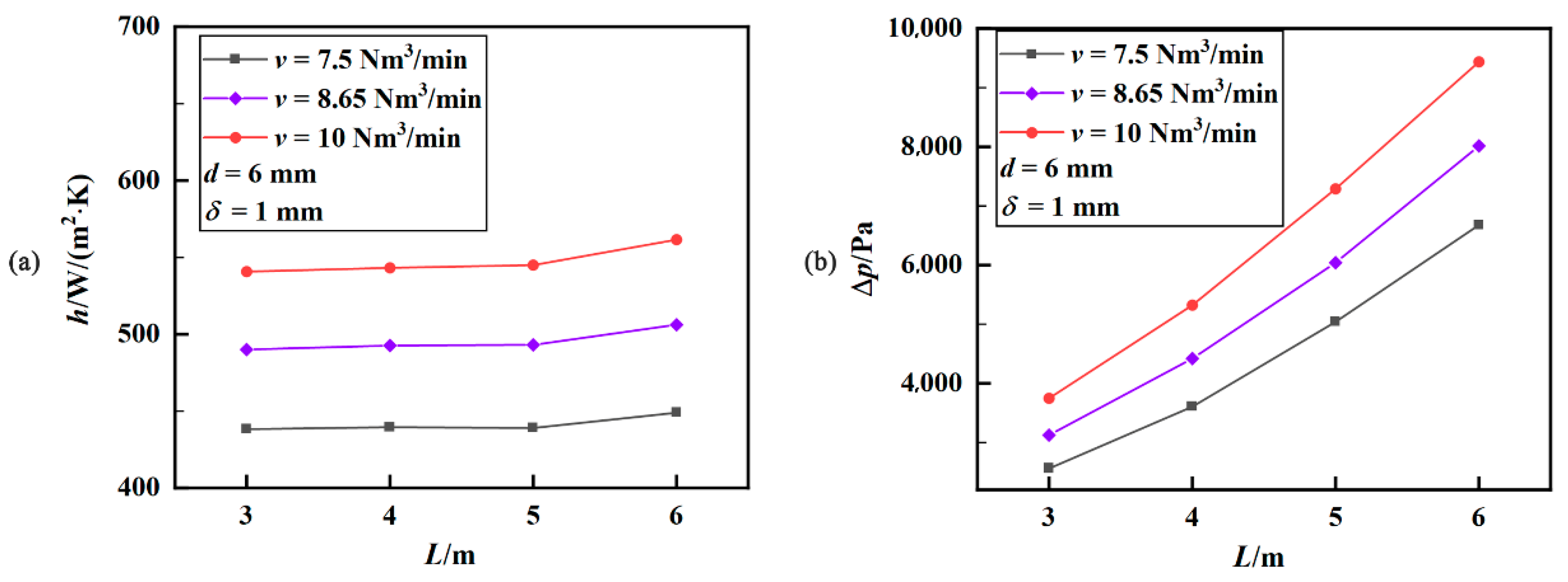
The length of the heating pipe is an important design parameter. The long downhole electric heater causes structural instability when the flow rate of nitrogen gas is high. Figure 7a–c show the changes of the heat-transfer coefficient, pressure drop, and comprehensive indexes of h/Δp1/3 versus the length of the heating tube, respectively. For the internal turbulent flow with a constant heat flux, the temperature difference between the wall and the fluid is expected to be constant, and the value of the heat-transfer coefficient is nearly independent of the length. In contrast, the pressure drop increases significantly when the length increases. As shown in Figure 7c, the comprehensive index of h/Δp1/3 decreases monotonically with the increase of the length. Figure 8 shows the corresponding temperature nephogram of the electric heater. It can be found that the wall temperature increases with the increase of the pipe length. The longer heating pipe will lead to a larger electrical resistance. Under the same electrical current, the heating power is larger, so the outlet temperature is expected to increase linearly with the length. Under the same heat transfer coefficient, the wall temperature increases correspondingly, as seen in Figure 7d.
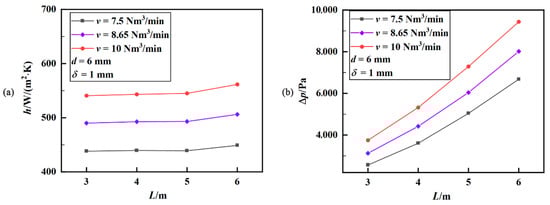
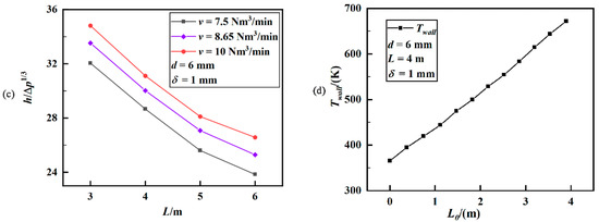
Figure 7.
Heat transfer and flow performance versus flow rate and the length of heating pipe: (a) h, (b) Δp, and (c) h/Δp1/3. (d) The variation of the wall temperature along the length of the heating pipe; the flow rate is G = 10 Nm3/min.

Figure 8.
Temperature nephogram of the electric heater at different lengths of heating pipes. In the simulation, the flow rate is G = 10 Nm3/min, tube diameter is d = 6 mm, and tube thickness is δ = 1 mm.
3.3. Effect of Inlet Flow Rate
The inlet flow rate is another important operation parameter in the downhole electric heater. On the one hand, the large flow rate can increase the heating capacity of the heater, making the kerogen decompose in a more efficient way. On the other, the large flow rate can decrease the outlet temperature of the heating fluid, and the pressure loss of the heater can increase dramatically. Figure 9a–c show the changes in the heat-transfer coefficient, pressure drop, and comprehensive indexes of h/Δp1/3 versus the flow rate, G, respectively. It is obvious that the larger the inlet flow rate is, the higher the heat-transfer coefficient and the pressure drop will be. As shown in Figure 9c, the comprehensive index of h/Δp1/3 increases monotonically with the increase of the mass flow rate. Therefore, under the studied conditions, the large flow rate benefits the performance of the heater. Figure 9d shows the temperature of the electric heater at different flow rates, and the corresponding temperature contours are shown in Figure 10. It can be found that the large flow rate will lead to a decrease in the temperature of the heating tube. Even for the largest flow rate, G = 10 Nm3/min, the outlet temperature of the fluid flow (~618 K) is still within the pyrolysis temperature range of the oil shale [18].
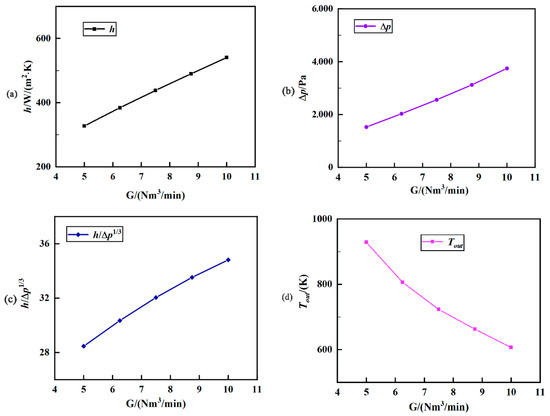
Figure 9.
Heat transfer, flow performance, and the outlet temperature versus flow rate: (a) h, (b) Δp, (c) h/Δp1/3, and (d) Tout. In this calculation, the inner diameter, thickness, and length of the heating pipes are d = 6 mm, δ =1 mm, and L = 3 m, respectively.
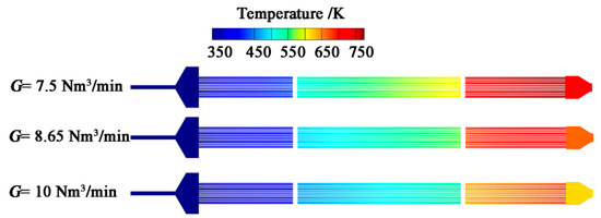
Figure 10.
Temperature nephogram of the electric heater at different flow rates.
3.4. Compared with Helical-Baffled Electric Heaters
The downhole electric heaters with continuous helical baffles have been proposed [9,10,11,12,13,14,15,16,21,22], which are designed to decrease the dead zones upside of the baffle. Table 2 compares these two typical working conditions for the helical-baffled electric heater [21] and the present tubular heater. In the comparison, the same heating power (120 kW), operation pressure (0.47 MPa), and flow rate (19.05 Nm3/min) of the compressed nitrogen gas are ensured. Although the heat-transfer area of the bare tubular heater is about half of the extended fins, the heat-transfer coefficient of the inner tube flow is almost ten times larger. Correspondingly, the thermal resistance is much smaller, and a higher outlet temperature is expected. Due to the high flow rate inside the small tube, the pressure drop is three orders larger than that of the helical-baffled electric heater. To decompose the oil shale featured by impermeable sedimentary rocks, a high heating flow rate is not necessary, especially during the initial heating stage. As shown in Figure 9d, the heating power and the flow rate can be conveniently adjusted to match the different heating requirements. Finally, the comprehensive index of the tubular electric heater is 40% higher than that of Wang et al. [21] under the same working condition, indicating that the present tubular electric heater is a promising candidate for the oil shale in situ resorting.
Table 2.
Heat-transfer performances for the helical-baffled electric heater and the present design.
4. Conclusions
In this paper, a downhole electric resistive heater was proposed for the oil-shale in situ resorting. Compared with the conventional armored electric heaters as the external fluid flows around a bundle of heating pipes, in the present electric heater, the heating fluid flows parallelly inside different heating tubes. The simulation results verify that the novel tubular electric heater has the following advantages: (1) The convective transfer coefficient is larger than 300 W/m2 K, which is much larger than the conductive heating and the armored electric heater. (2) The outlet temperature of the heating fluid can reach up to about 900 °C without the complex structure of enhanced fins. (3) The comprehensive index can be 40% higher than that of the armored electric heater with extended fins, and the heating power and the flow rate can be conveniently adjusted to match different downhole heating requirements.
Author Contributions
Y.C. contributed to methodology, software, validation, investigation, and writing—original draft preparation; H.Z. contributed to methodology, data curation, writing—reviewing and editing, and project administration; J.W. contributed to conceptualization, supervision, writing—reviewing and editing, and funding acquisition; H.C. contributed to methodology and software; J.Z. contributed to methodology, funding acquisition, and writing—reviewing and editing. All authors have read and agreed to the published version of the manuscript.
Funding
This research was funded by the National Natural Science Foundation of China (Nos. 51876041 and 52004304), the Opening Project of the State Key Laboratory of Shale Oil and Gas Enrichment Mechanisms and Effective Development (No. P20066), and the Fundamental Research Funds for the Central Universities.
Institutional Review Board Statement
Not applicable.
Informed Consent Statement
Not applicable.
Conflicts of Interest
The authors declare no conflict of interest.
References
- Jiang, X.; Han, X.; Cui, Z. New technology for the comprehensive utilization of Chinese oil shale resources. Energy 2007, 32, 772–777. [Google Scholar] [CrossRef]
- Yang, Q.; Qian, Y.; Kraslawski, A.; Zhou, H.; Yang, S. Framework for advanced exergoeconomic performance analysis and optimization of an oil shale retorting process. Energy 2016, 109, 62–76. [Google Scholar] [CrossRef]
- Wang, S.; Jiang, X.; Han, X.; Tong, J. Investigation of Chinese oil shale resources comprehensive utilization performance. Energy 2012, 42, 224–232. [Google Scholar] [CrossRef]
- Brandt, A.R. Converting oil shale to liquid fuels: Energy inputs and greenhouse gas emissions of the Shell in situ conversion process. Environ. Sci. Technol. 2008, 42, 7489–7495. [Google Scholar] [CrossRef] [PubMed]
- Kang, Z.; Zhao, Y.; Yang, D.; Tian, L.; Li, X. A pilot investigation of pyrolysis from oil and gas extraction from oil shale by in-situ superheated steam injection. J. Pet. Sci. Eng. 2020, 186, 106785. [Google Scholar] [CrossRef]
- Branch, M.C. In-situ combustion retorting of oil shale. Prog. Energy Combust. Sci. 1979, 5, 193–206. [Google Scholar] [CrossRef]
- Crawford, P.M.; Killen, J.C. New challenges and directions in oil shale development technologies. ACS Symp. Ser. 2010, 1032, 21–60. [Google Scholar]
- Huang, C.; Hou, H.; Yu, G.; Zhang, L.; Hu, E. Energy solutions for producing shale oil: Characteristics of energy demand and economic analysis of energy supply options. Energy 2020, 192, 116601–116603. [Google Scholar] [CrossRef]
- Wang, Z.; Lü, X.; Li, Q.; Sun, Y.; Wang, Y.; Deng, S.; Guo, W. Downhole electric heater with high heating efficiency for oil shale exploitation based on a double-shell structure. Energy 2020, 211, 118539. [Google Scholar] [CrossRef]
- Gu, H.; Chen, Y.; Wu, J.; Yang, S. Numerical study on performances of small incline angle helical baffle electric heaters with axial separation. Appl. Therm. Eng. 2017, 126, 963–975. [Google Scholar] [CrossRef]
- Guo, W.; Wang, Z.; Sun, Z.; Sun, Y.; Lü, X.; Deng, S.; Qu, L.; Yuan, W.; Li, Q. Experimental investigation on performance of downhole electric heaters with continuous helical baffles used in oil shale in-situ pyrolysis. Appl. Therm. Eng. 2019, 147, 1024–1035. [Google Scholar] [CrossRef]
- Yang, S.; Chen, Y.; Wu, J.; Gu, H. Influence of baffle configurations on flow and heat transfer characteristics of unilateral type helical baffle heat exchangers. Appl. Therm. Eng. 2018, 13, 739–748. [Google Scholar] [CrossRef]
- Wang, M.C.; Chen, Y.P.; Wu, J.F.; Dong, C. Numerical simulation of the heat transfer performance of trisection helical baffled electric heaters. Numer. Heat Transf. Part A Appl. 2016, 69, 85–96. [Google Scholar] [CrossRef]
- Tang, H.; Chen, Y.; Wu, J.; Yang, S. Numerical investigation of the performances of axial separation helical baffle heat exchangers. Energy Convers. Manag. 2016, 126, 400–410. [Google Scholar] [CrossRef]
- Delouei, A.A.; Sajjadi, H.; Mohebbi, R.; Izadi, M. Experimental study on inlet turbulent flow under ultrasonic vibration: Pressure drop and heat transfer enhancement. Ultrason. Sonochem. 2019, 51, 151–159. [Google Scholar] [CrossRef] [PubMed]
- Delouei, A.A.; Atashafrooz, M.; Sajjadi, H.; Karimnejad, S. The thermal effects of multi-walled carbon nanotube concentration on an ultrasonic vibrating finned tube heat exchanger. Int. Commun. Heat Mass Trans. 2022, 135, 106098. [Google Scholar] [CrossRef]
- Kathrein, H.; Freund, F. Electrical conductivity of magnesium oxide single crystal below 1200 K. J. Phys. Chem. Solids 1983, 44, 177–186. [Google Scholar] [CrossRef]
- Ogunsola, O.I.; Hartstein, A.; Ogunsola, O. Oil Shale: A Solution to the Liquid Fuel Dilemma. In ACS Symposium Series; American Chemical Society: Washington, DC, USA, 2013; Volume 1032. [Google Scholar]
- Wang, X.; Ni, Q.H.; Zhou, H.; Kong, Q.P. Cyclic creep behavior of a nickel base alloy. Mater. Sci. Eng. A 1990, 123, 207–211. [Google Scholar] [CrossRef]
- Salameh, T.; Tawalbeh, M.; Juaidi, A.; Abdallah, R.; Hamid, A. A novel three-dimensional numerical model for PV/T water system in hot climate region. Renew. Energy 2021, 164, 1320–1333. [Google Scholar] [CrossRef]
- Wang, M.C.; Chen, Y.P.; Wu, J.F.; Dong, C. Heat transfer enhancement of folded helical baffle electric heaters with one-plus-two U-tube units. Appl. Therm. Eng. 2016, 102, 586–595. [Google Scholar] [CrossRef]
- Wang, Z.; Guo, W.; Sun, Y.; Li, Q.; Deng, S.; Zhang, P.; Zhao, S.; Chen, Q.; Liu, Z. Fluid Electric Heater in Pit. Chinese Patent CN CN208168849U, 30 November 2018. [Google Scholar]


Publisher’s Note: MDPI stays neutral with regard to jurisdictional claims in published maps and institutional affiliations. |
© 2022 by the authors. Licensee MDPI, Basel, Switzerland. This article is an open access article distributed under the terms and conditions of the Creative Commons Attribution (CC BY) license (https://creativecommons.org/licenses/by/4.0/).