
Finite Element Analysis of Punching Shear of Reinforced Concrete Slab–Column Connections with Shear Reinforcement


Abstract
:1. Introduction
2. Finite Element Simulation
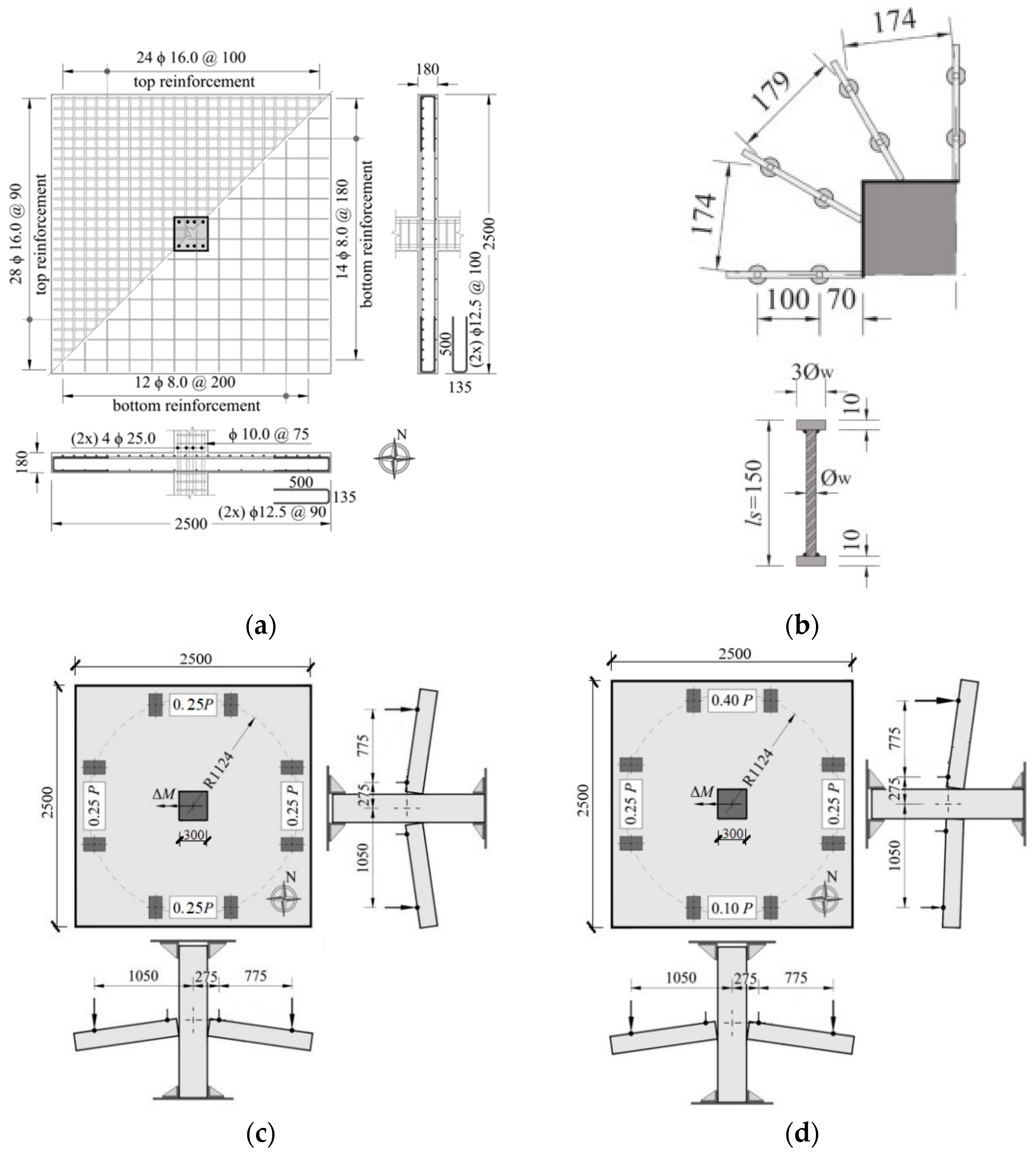
2.1. Test Specimens
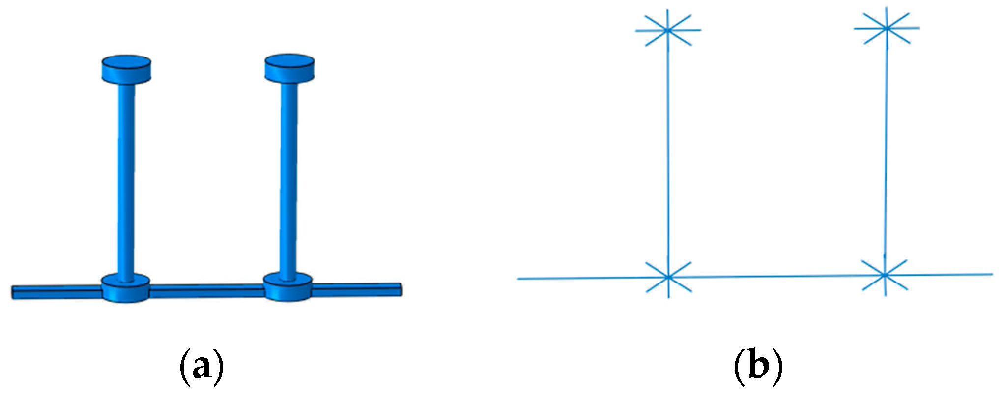
2.2. Methodology
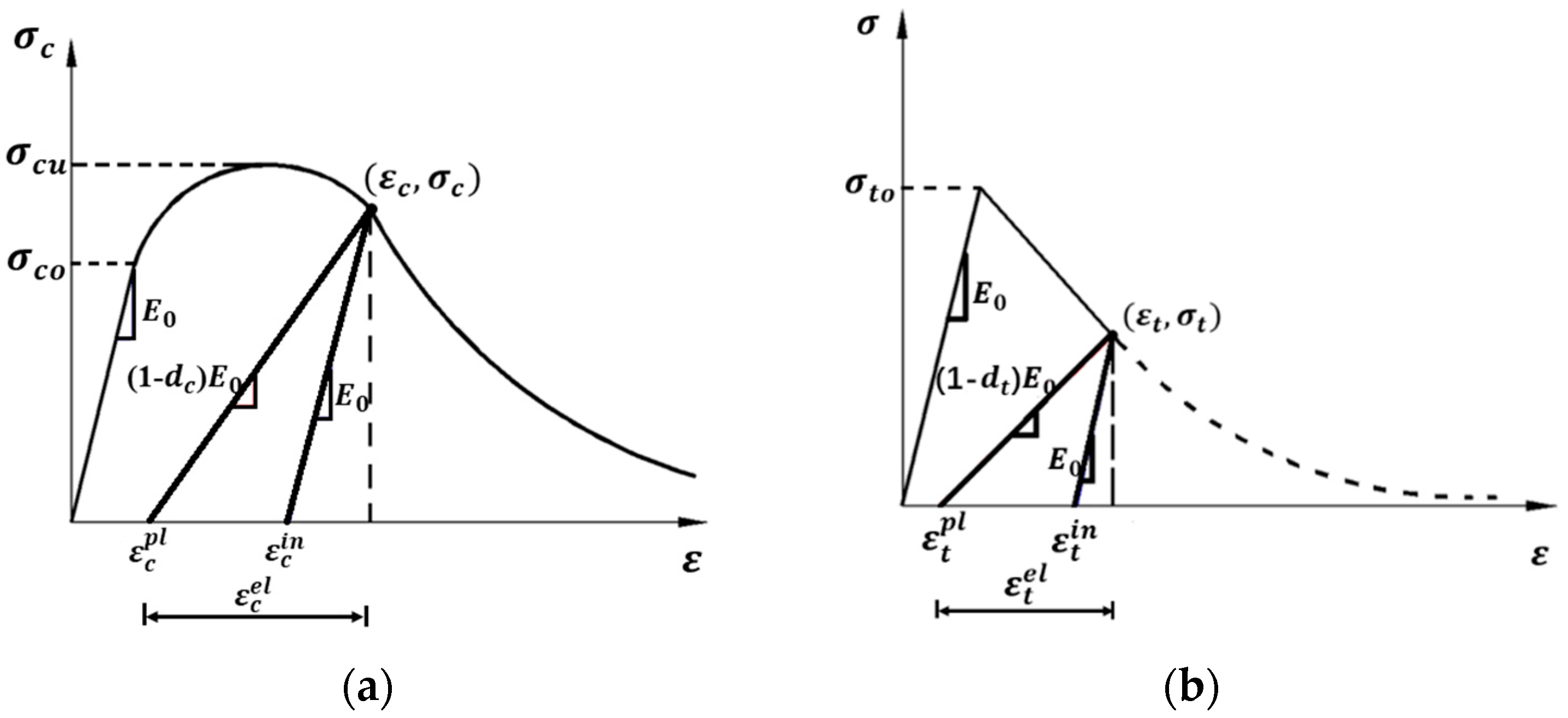
2.3. Concrete Damage Plasticity Model
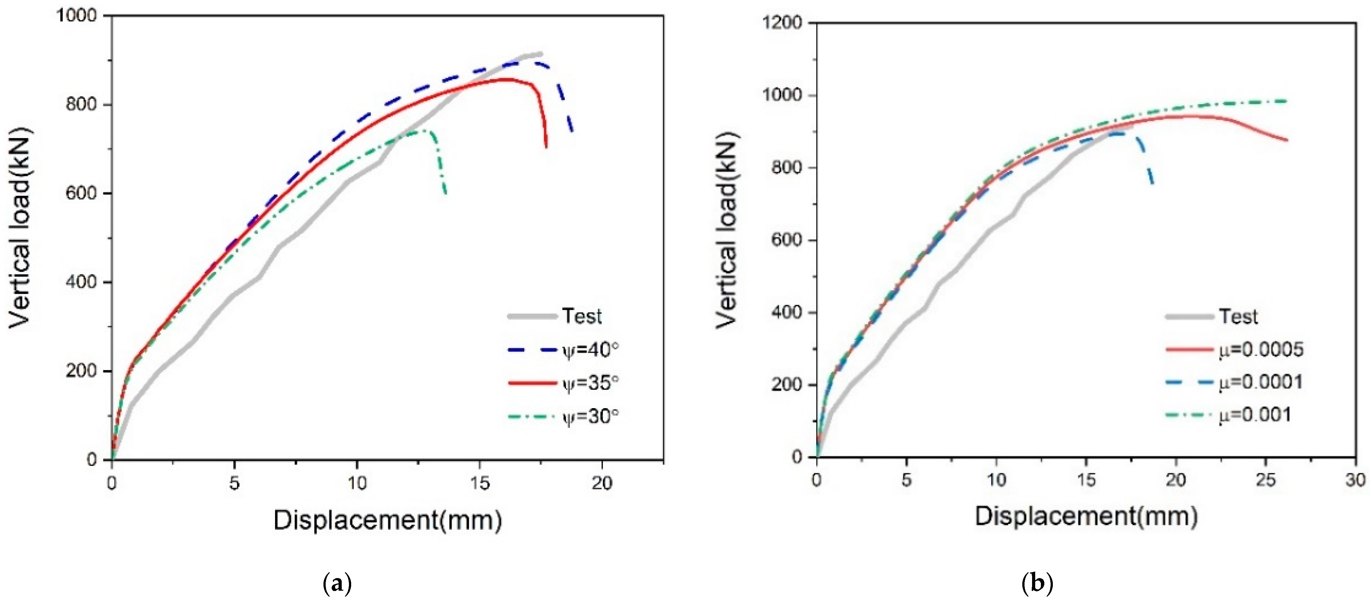
2.4. Calibration of CDP Parameters
3. Finite Element Model Validation
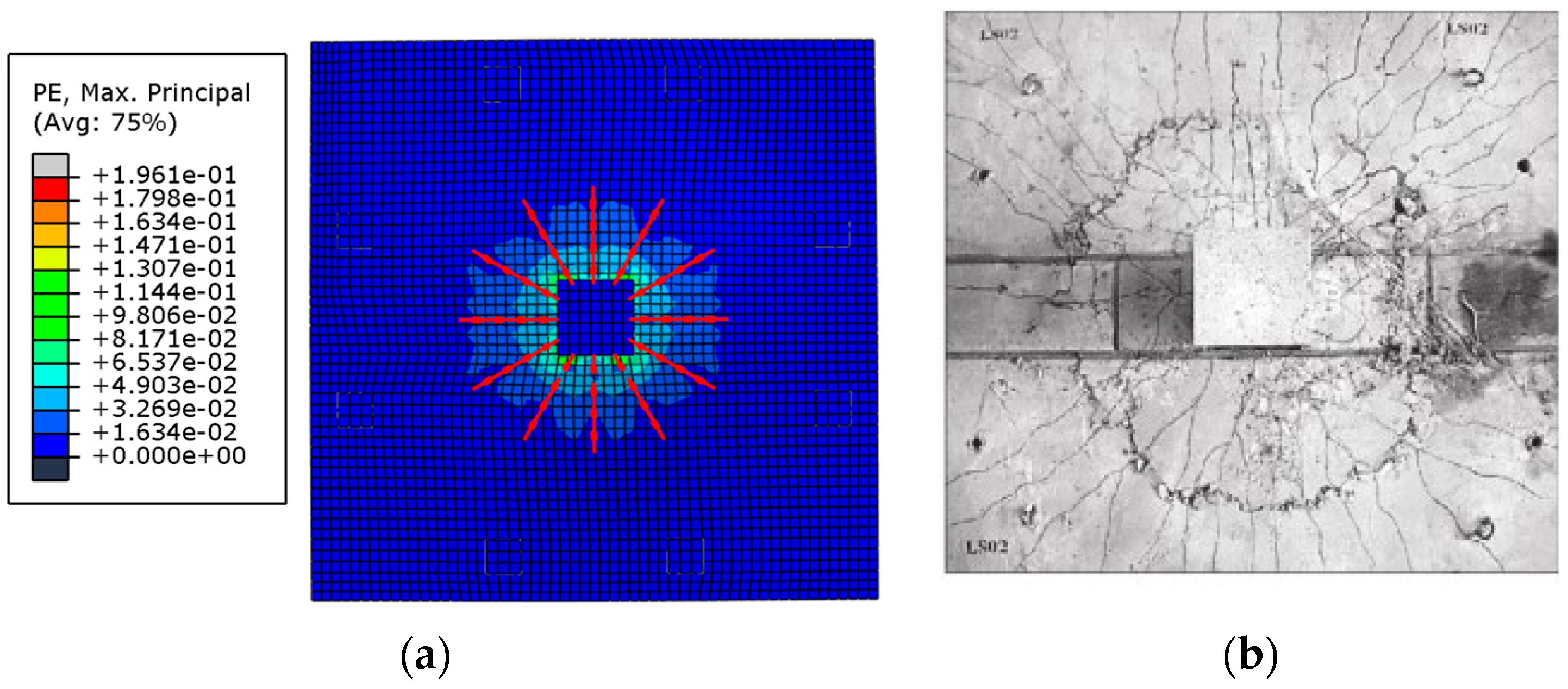
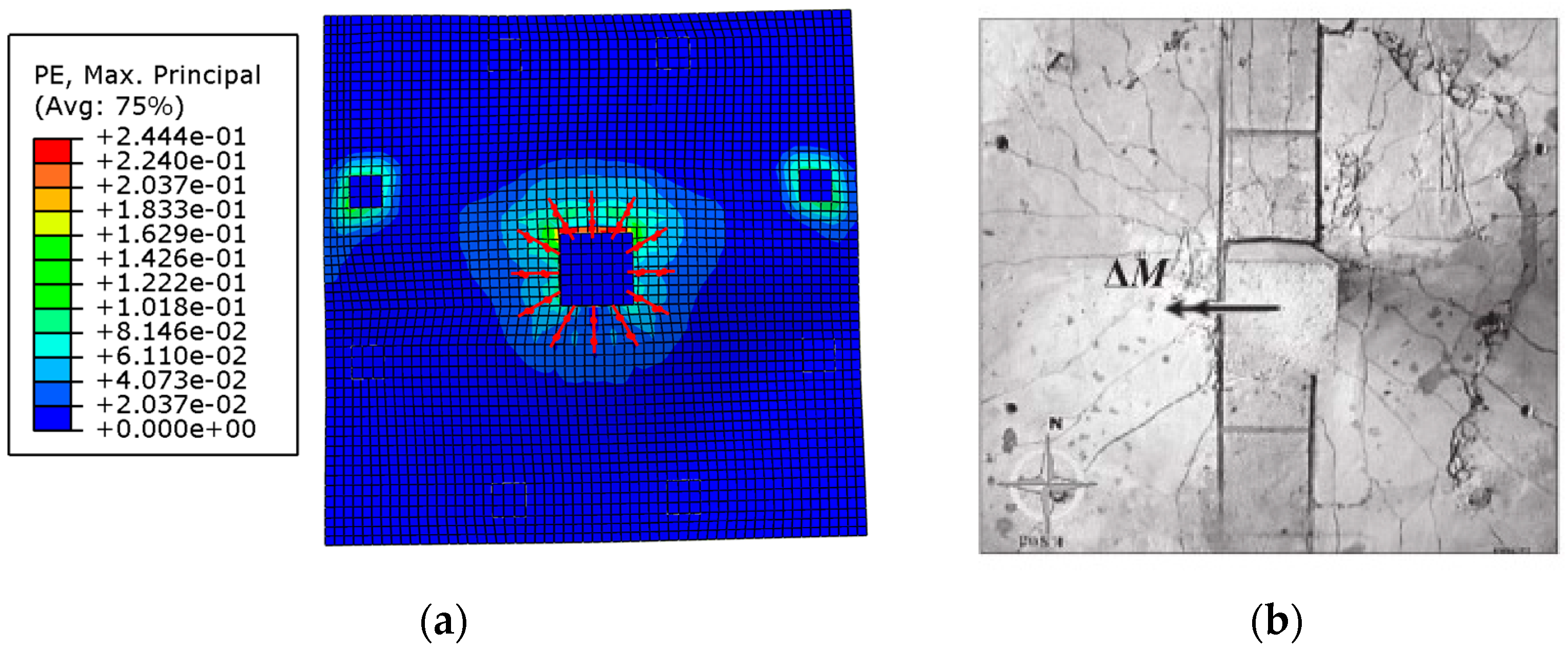
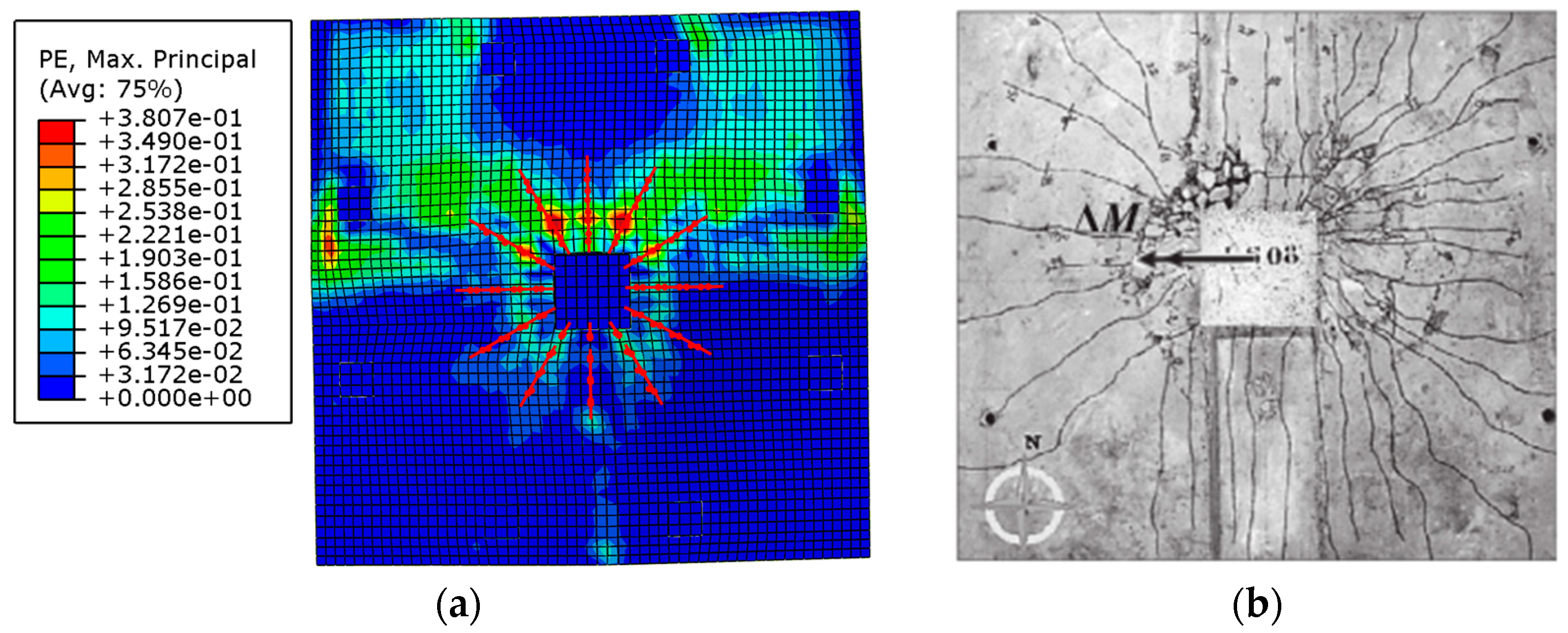
3.1. Crack Pattern
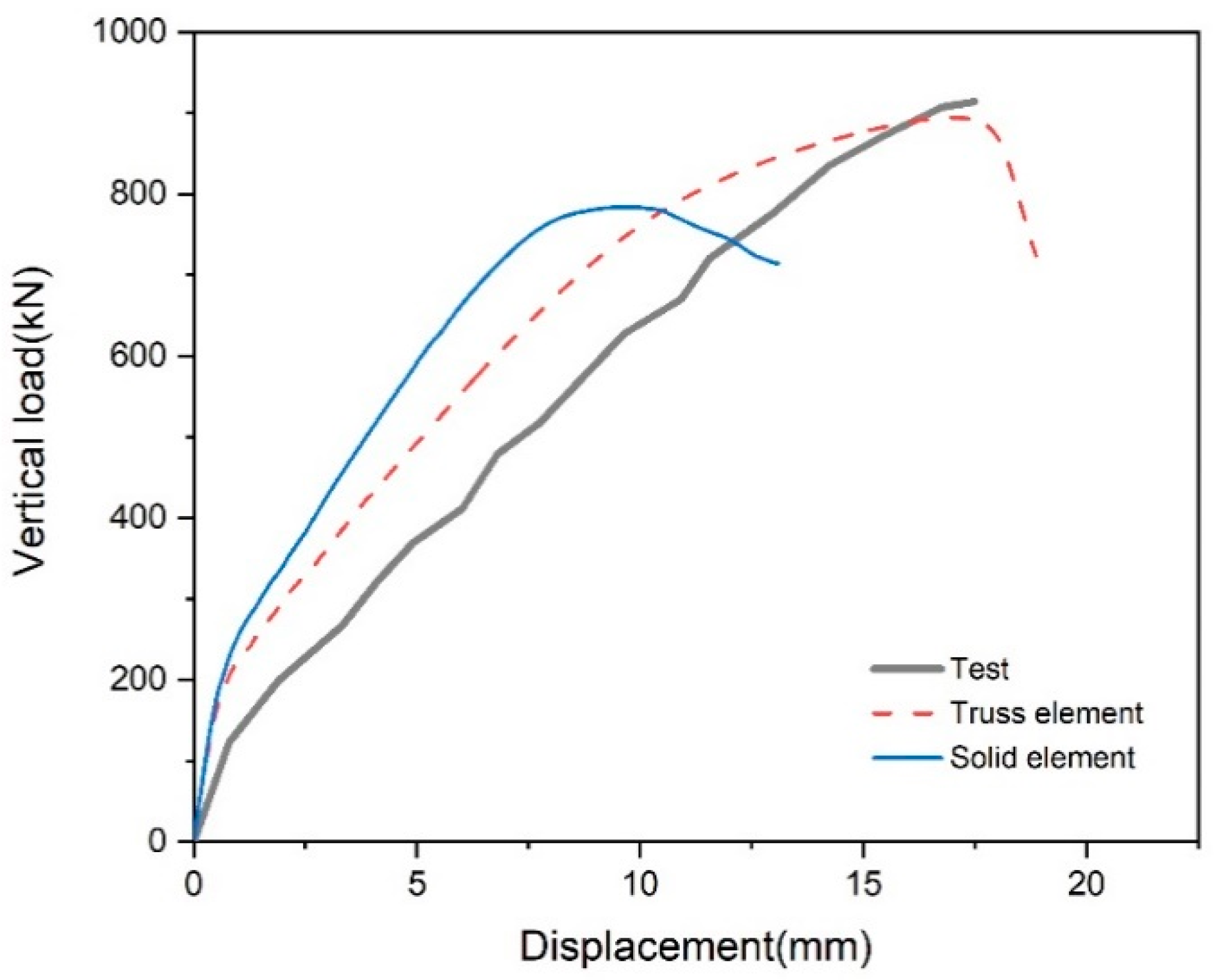
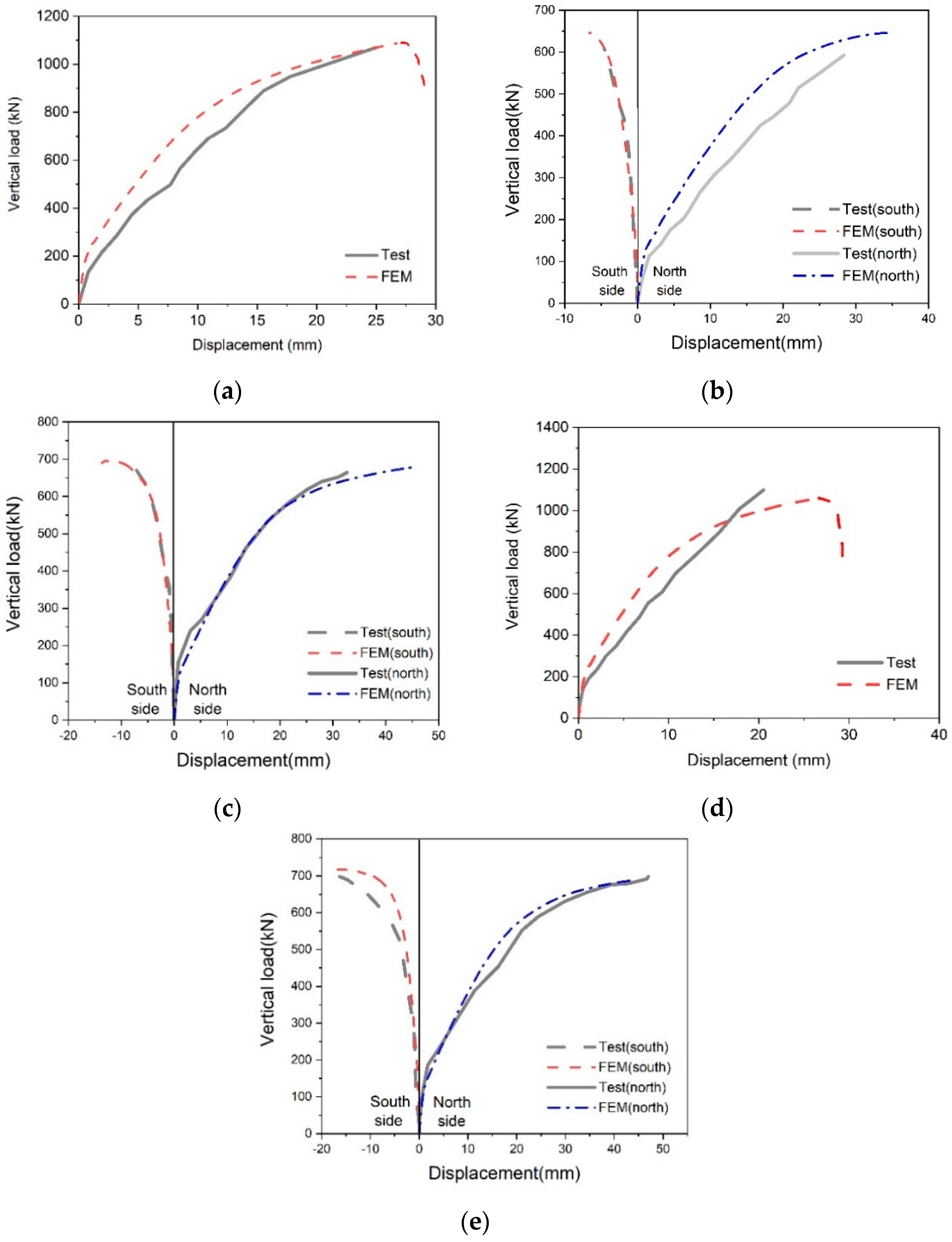
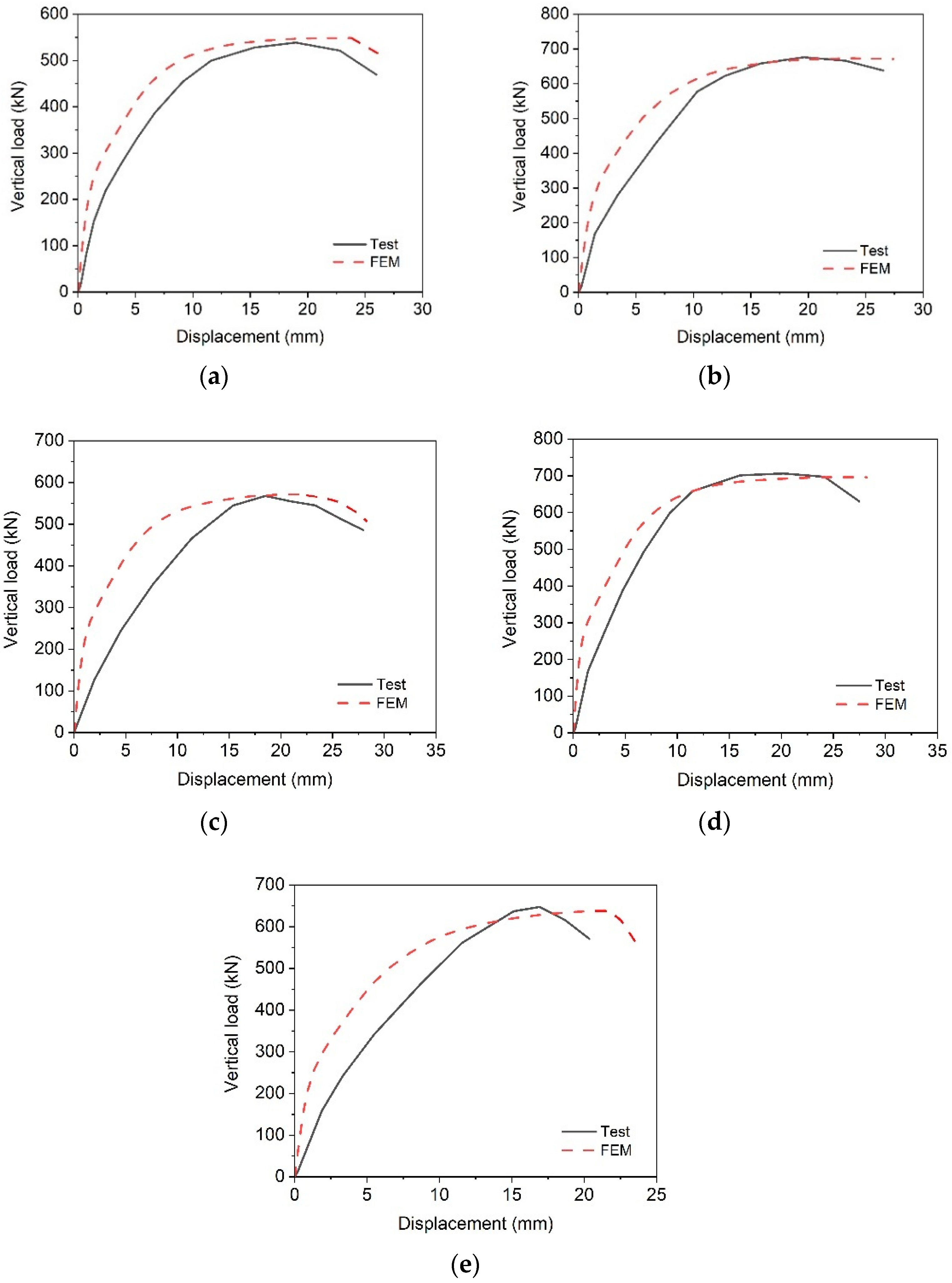
3.2. Load–Deflection Response
4. Finite Element Analysis Results and Discussion
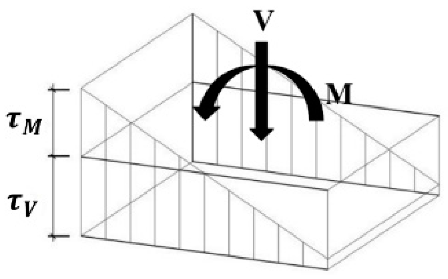
4.1. Average Shear Stress in the Critical Section
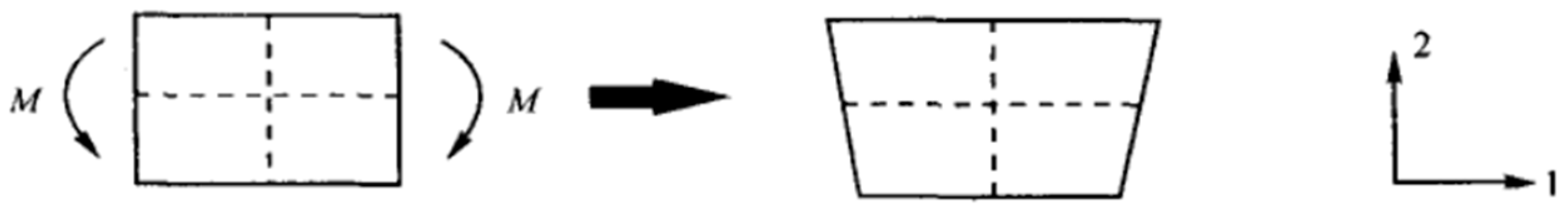
4.2. Coefficient of the Bending Moment Transferred by the Eccentric Shear Force
5. Conclusions
Author Contributions
Funding
Institutional Review Board Statement
Informed Consent Statement
Data Availability Statement
Acknowledgments
Conflicts of Interest
Appendix A

| Strength * | Concrete Strength Grade | |||||||||||||
|---|---|---|---|---|---|---|---|---|---|---|---|---|---|---|
| C15 | C20 | C25 | C30 | C35 | C40 | C45 | C50 | C55 | C60 | C65 | C70 | C75 | C80 | |
| , MPa | 1.27 | 1.54 | 1.78 | 2.01 | 2.20 | 2.39 | 2.51 | 2.64 | 2.74 | 2.85 | 2.93 | 2.99 | 3.05 | 3.11 |
| C15 | C20 | C25 | C30 | C35 | C40 | C45 | C50 | C55 | C60 | C65 | C70 | C75 | C80 | |
|---|---|---|---|---|---|---|---|---|---|---|---|---|---|---|
| 2.20 | 2.55 | 2.80 | 3.00 | 3.15 | 3.25 | 3.35 | 3.45 | 3.55 | 3.60 | 3.65 | 3.70 | 3.75 | 3.80 |
Appendix B
| x | σ (MPa) | εcin | d (Damage Factor) |
|---|---|---|---|
| 1 | 47.5 | 0 | 0 |
| 1.2 | 44.05401755 | 0.001048737 | 0.267557159 |
| 1.4 | 37.45498901 | 0.001607639 | 0.374737446 |
| 1.6 | 31.08645197 | 0.002160191 | 0.467159548 |
| 1.8 | 25.89451431 | 0.002680325 | 0.541500112 |
| 2 | 21.85589911 | 0.003168683 | 0.600385772 |
| 2.2 | 18.73035207 | 0.003631883 | 0.647277445 |
| 2.4 | 16.2870195 | 0.004076288 | 0.685089756 |
| 2.6 | 14.3480681 | 0.004506795 | 0.716023997 |
| 2.8 | 12.78458397 | 0.004926958 | 0.741693172 |
| 3 | 11.50435808 | 0.005339316 | 0.763276066 |
| x | σ (MPa) | εtin | d (Damage Factor) |
|---|---|---|---|
| 1 | 2.9 | 0 | 0 |
| 1.2 | 2.53996257 | 0.00006863 | 0.2894486 |
| 1.4 | 2.079222415 | 0.000104423 | 0.4048055 |
| 1.6 | 1.717849378 | 0.000137481 | 0.4939365 |
| 1.8 | 1.451784456 | 0.000167913 | 0.5613812 |
| 2 | 1.254346961 | 0.000196454 | 0.613218 |
| 2.2 | 1.104316821 | 0.000223689 | 0.6539746 |
| 2.4 | 0.987361044 | 0.000250013 | 0.6867401 |
| 2.6 | 0.894017368 | 0.000275686 | 0.7136094 |
| 2.8 | 0.817961603 | 0.000300883 | 0.7360268 |
| 3 | 0.754871444 | 0.000325723 | 0.75501 |
| x | σ (MPa) | εcin | d (Damage Factor) |
|---|---|---|---|
| 1 | 22.8 | 0 | 0 |
| 1.2 | 22.11975209 | 0.001088221 | 0.364474397 |
| 1.4 | 20.62529509 | 0.001442294 | 0.431841361 |
| 1.6 | 18.88069762 | 0.001804705 | 0.491509816 |
| 1.8 | 17.16826615 | 0.002166044 | 0.542848117 |
| 2 | 15.60260504 | 0.002522491 | 0.586555607 |
| 2.2 | 14.21555962 | 0.002872983 | 0.62372602 |
| 2.4 | 13.00295496 | 0.003217661 | 0.655452617 |
| 2.6 | 11.94721089 | 0.00355711 | 0.682692646 |
| 2.8 | 11.02745329 | 0.003892027 | 0.706240348 |
| 3 | 10.22367193 | 0.004223077 | 0.726739806 |
| x | σ (MPa) | εtin | d (Damage Factor) |
|---|---|---|---|
| 1 | 2 | 0 | 0 |
| 1.2 | 1.873677919 | 0.0000509539 | 0.2579017 |
| 1.4 | 1.683850766 | 0.0000761831 | 0.3486831 |
| 1.6 | 1.506813457 | 0.000100986 | 0.4236659 |
| 1.8 | 1.356433364 | 0.0001249 | 0.4844538 |
| 2 | 1.231527094 | 0.000147966 | 0.5339725 |
| 2.2 | 1.127781845 | 0.000170325 | 0.5747877 |
| 2.4 | 1.040938938 | 0.000192122 | 0.6088786 |
| 2.6 | 0.96749296 | 0.000213472 | 0.6377221 |
| 2.8 | 0.904709908 | 0.000234466 | 0.6624172 |
| 3 | 0.850489121 | 0.000255175 | 0.683788 |
References
- Elstner, R.C.; Hognestad, E. Shearing strength of reinforced concrete slabs. ACI 1956, 53, 29–58. [Google Scholar]
- Moe, J. Shearing Strength of Reinforced Concrete Slabs and Footings under Concentrated Loads; Bulletin D47; Portland Cement Association, Research and Development Laboratories: Skokie, IL, USA, 1961. [Google Scholar]
- Regan, P.E. Design for punching shear. Struct. Eng. J. 1974, 52, 197–207. [Google Scholar]
- Regan, P.E.; Braestrup, M.W. Punching Shear in Reinforced Concrete—A State-of-the-Art Report; Bulletin d’Information No. 168; Comité Euro-International du Béton: Lausanne, Switzerland, 1985. [Google Scholar]
- Hanson, N.W.; Hanson, J.M. Shear and Moment Transfer Between Concrete Slabs and Columns. J. PCA Res. Dev. Lab. 1968, 10, 2–16. [Google Scholar]
- ACI Committee 318. Building Code Requirements for Structural Concrete (ACI 318-70) and Commentary; American Concrete Institute: Farmington Hills, MI, USA, 1970. [Google Scholar]
- Chen, W.F.; Han, D.J. Plasticity for Structural Engineers; Springer: New York, NY, USA, 1988. [Google Scholar]
- Simo, J.C.; Ju, J.W. Strain- and stress-based continuum damage models–I. Formulation. Int. J. Solids Struct. 1987, 23, 821–840. [Google Scholar] [CrossRef]
- Grassl, P.; Jirásek, M. Damage-plastic model for concrete failure. Int. J. Solids Stuct. 2006, 43, 7166–7196. [Google Scholar] [CrossRef]
- Park, H.; Choi, K. Improved strength model for interior flat plate–column connections subject to unbalanced moment. J. Struct. Eng. 2006, 132, 694–704. [Google Scholar] [CrossRef]
- ABAQUS. Analysis User’s Manual 6.12-3; Dassault Systems Simulia Corp.: Providence, RI, USA, 2010. [Google Scholar]
- Xiong, J.; Ding, L.; Tian, Q. Calculation method and experimental validation of concrete damage plasticity model parameters. J. Nanchang Univ. 2019, 1, 21–26. [Google Scholar] [CrossRef]
- Peng, X.-j.; Yu, A.-l.; Fang, Y.-z. Parametric analysis of concrete damage plasticity model. J. Suzhou Inst. Sci. Technol. 2010, 3, 40–43. [Google Scholar]
- Li, Q.; Kuang, Y.; Guo, W. Calculation of CDP model parameters and validation of the taking method. J. Zhengzhou Univ. 2021, 2, 43–48. [Google Scholar] [CrossRef]
- Ferreira, M.D.; Oliveira, M.H.; Sales, G.; Melo, S.A. Tests on the Punching Resistance of Flat Slabs with Unbalanced Moments. Eng. Struct. 2019, 196, 109311. [Google Scholar] [CrossRef]
- Tian, J.; Xu, K. Experimental research on concrete slab-column joints with punching shear anchor bolts. J. North. Jiaotong Univ. 1999, 6, 73–77. [Google Scholar]
- Genikomsou, A. Nonlinear Finite Element Analysis of Punching Shear of Reinforced Concrete Slab-Column Connection. Ph.D. Thesis, University of Waterloo, Waterloo, ON, Canada, 2015. Available online: http://hdl.handle.net/10012/10112 (accessed on 1 June 2021).
- Lubliner, J.; Oliver, J.; Oller, S.; Onate, E. Aplastic-damage Model for Concrete. Int. J. Solids Struct. 1989, 25, 299–326. [Google Scholar] [CrossRef]
- GB50010-2010; Code for Design of Concrete Structures. National Standard of the People’s Republic of China: Beijing, China, 2011. (In Chinese)
- Wu, Y.J.; Li, J.; Rui, F. An Energy Release Rate-based Plastic-damage Model for Concrete. Int. J. Solids Struct. 2006, 43, 583–612. [Google Scholar] [CrossRef]
- European Committee for Standardization. Design of Concrete Structures–Part 1-1: GENERAL Rules and Rules for Buildings; EUROCODE 2: Brussels, Belgium, 2004. [Google Scholar]
- ACI Committee 318. ACI Building Code Requirements for Structural Concrete (ACI 318-19) and Commentary (ACI 318R-19); American Concrete Institute: Farmington Hills, MI, USA, 2019. [Google Scholar]
- Guo, J.; Xu, B. Study on the Value of Damage Factor and Application of Concrete Damage Plasticity Model. Gansu J. Sci. 2019, 88–92. [Google Scholar] [CrossRef]
- Yao, F.; Guan, Q.; Wang, P. Simulation Analysis of Damage Factors Based on ABAQUS Plastic Damage Model. Struct. Eng. 2019, 5, 76–81. [Google Scholar] [CrossRef]
- Sidoroff, F. Description of Anisotropic Damage Application to Elasticity. In Physical Non-Linearities in Structural Analysis; Springer: Berlin/Heidelberg, Germany, 1981. [Google Scholar]


| Specimen | Type of Load 1 | Concrete | Flexural Reinforcement | Shear Studs | ||||
|---|---|---|---|---|---|---|---|---|
| , MPa | , MPa | , GPa | (%) | Studs 2 | , MPa | , GPa | ||
| S1 | C | 48.3 | 540 | 213 | 1.46 | 535 | 211 | |
| S3 | E | 50.3 | 1.46 | |||||
| S2 | C | 49.4 | 1.48 | |||||
| S4 | E | 49.2 | 1.48 | |||||
| S7 | C | 48.9 | 1.48 | 518 | 204 | |||
| S8 | E | 48.4 | 1.47 | |||||
| Specimen | Distance of the First Row of Studs from the Column Surface, mm | Studs’ Spacing, mm | Number of Studs on Each Steel Plate | |
|---|---|---|---|---|
| P1 | 24 | 68 | 101 | 4 |
| P2 | 24 | 68 | 75 | 7 |
| P3 | 25 | 47 | 68 | 9 |
| P4 | 25.1 | 54 | 78 | 9 |
| P5 | 25.3 | 47 | 68 | 7 |
| Experience | Specimen | Shear Studs, Number/Diameter | M/V | M, kN·m | V, kN | Average Shear Stress, MPa | |
|---|---|---|---|---|---|---|---|
| Ferreira et al. [15] | S1 | 2 studs/10 mm | 0 | 0 | 977 | 2.86 | 0 |
| S3 | 0.27 | 224 | 723 | 2.80 | 0.095 | ||
| 2-10-036 | 0.36 | 297 | 824 | 2.89 | 0.129 | ||
| 2-10-045 | 0.45 | 337 | 748 | 2.72 | 0.148 | ||
| 2-10-054 | 0.54 | 378 | 700 | 2.64 | 0.161 | ||
| S2 | 4 studs/10 mm | 0 | 0 | 1159 | 3.26 | 0 | |
| S4 | 0.27 | 265 | 687 | 3.31 | 0.096 | ||
| 4-10-036 | 0.36 | 339 | 942 | 3.29 | 0.127 | ||
| 4-10-045 | 0.45 | 345 | 766 | 2.85 | 0.155 | ||
| 4-10-054 | 0.54 | 383 | 709 | 2.75 | 0.169 | ||
| 6-10-0 | 6 studs/10 mm | 0 | 0 | 1160 | 3.23 | 0 | |
| 6-10-027 | 0.27 | 270 | 999 | 3.32 | 0.099 | ||
| 6-10-036 | 0.36 | 346 | 960 | 3.36 | 0.128 | ||
| 6-10-045 | 0.45 | 347 | 770 | 2.96 | 0.161 | ||
| 6-10-054 | 0.54 | 389 | 721 | 2.82 | 0.171 | ||
| 2-12.5-0 | 2 studs/12.5 mm | 0 | 0 | 948 | 2.87 | 0 | |
| 2-12.5-027 | 0.27 | 239 | 884 | 2.96 | 0.092 | ||
| 2-12.5-036 | 0.36 | 306 | 849 | 2.97 | 0.128 | ||
| 2-12.5-045 | 0.45 | 344 | 764 | 2.77 | 0.147 | ||
| 2-12.5-054 | 0.54 | 380 | 704 | 2.70 | 0.166 | ||
| S7 | 4 studs/12.5 mm | 0 | 0 | 1142 | 3.14 | 0 | |
| S8 | 0.27 | 265 | 981 | 3.42 | 0.113 | ||
| 4-12.5-036 | 0.36 | 341 | 947 | 3.39 | 0.137 | ||
| 4-12.5-045 | 0.45 | 349 | 777 | 2.90 | 0.157 | ||
| 4-12.5-054 | 0.54 | 392 | 726 | 2.81 | 0.168 | ||
| 6-12.5-0 | 6 studs/12.5 mm | 0 | 0 | 1185 | 3.28 | 0 | |
| 6-12.5-027 | 0.27 | 276 | 1024 | 3.52 | 0.115 | ||
| 6-12.5-036 | 0.36 | 359 | 997 | 3.52 | 0.141 | ||
| 6-12.5-045 | 0.45 | 355 | 788 | 3.00 | 0.163 | ||
| 6-12.5-054 | 0.54 | 399 | 738 | 2.88 | 0.171 | ||
| 2-8-0 | 2 studs/8 mm | 0 | 0 | 901 | 2.67 | 0 | |
| 2-8-027 | 0.27 | 211 | 783 | 2.62 | 0.082 | ||
| 2-8-036 | 0.36 | 274 | 761 | 2.65 | 0.116 | ||
| 2-8-045 | 0.45 | 304 | 675 | 2.55 | 0.140 | ||
| 2-8-054 | 0.54 | 341 | 631 | 2.51 | 0.156 | ||
| 4-8-0 | 4 studs/8 mm | 0 | 0 | 1047 | 3.04 | 0 | |
| 4-8-027 | 0.27 | 260 | 962 | 3.15 | 0.092 | ||
| 4-8-036 | 0.36 | 332 | 923 | 3.12 | 0.125 | ||
| 4-8-045 | 0.45 | 339 | 754 | 2.71 | 0.144 | ||
| 4-8-054 | 0.54 | 381 | 706 | 2.62 | 0.167 | ||
| 6-8-0 | 6 studs/8 mm | 0 | 0 | 1108 | 3.08 | 0 | |
| 6-8-027 | 0.27 | 261 | 966 | 3.17 | 0.093 | ||
| 6-8-036 | 0.36 | 334 | 926.5 | 3.15 | 0.127 | ||
| 6-8-045 | 0.45 | 339 | 754 | 2.68 | 0.161 | ||
| 6-8-054 | 0.54 | 381 | 705 | 2.60 | 0.165 | ||
| 2-15-0 | 2 studs/15 mm | 0 | 0 | 991 | 2.91 | 0 | |
| 2-15-027 | 0.27 | 242 | 897 | 3.02 | 0.095 | ||
| 2-15-036 | 0.36 | 313 | 869 | 3.01 | 0.134 | ||
| 2-15-045 | 0.45 | 348 | 773 | 2.82 | 0.149 | ||
| 2-15-054 | 0.54 | 387 | 717 | 2.73 | 0.174 | ||
| 4-15-0 | 4 studs/15 mm | 0 | 0 | 1158 | 3.25 | 0 | |
| 4-15-027 | 0.27 | 276 | 1023 | 3.54 | 0.119 | ||
| 4-15-036 | 0.36 | 355 | 985 | 3.52 | 0.136 | ||
| 4-15-045 | 0.45 | 355 | 789 | 2.90 | 0.151 | ||
| 4-15-054 | 0.54 | 396 | 733 | 2.79 | 0.174 | ||
| 6-15-0 | 6 studs/15 mm | 0 | 0 | 1203 | 3.39 | 0 | |
| 6-15-027 | 0.27 | 306 | 1132 | 3.68 | 0.128 | ||
| 6-15-036 | 0.36 | 387 | 1076 | 3.73 | 0.137 | ||
| 6-15-045 | 0.45 | 383 | 850 | 3.05 | 0.164 | ||
| 6-15-054 | 0.54 | 423 | 784 | 2.95 | 0.181 | ||
| J. Tian and K.B. Xu [16] | P1 | 4 studs/s = 101 mm | 0 | 0 | 541 | 2.08 | 0 |
| P1-10-050 | 0.50 | 196 | 399 | 2.81 | 0.125 | ||
| P1-10-068 | 0.68 | 199 | 296 | 2.71 | 0.177 | ||
| P1-10-165 | 1.65 | 229 | 139 | 2.63 | 0.259 | ||
| P2 | 7 studs/s = 75 mm | 0 | 0 | 672 | 2.42 | 0 | |
| P2-10-051 | 0.51 | 230 | 450 | 2.96 | 0.094 | ||
| P2-10-071 | 0.71 | 231 | 325 | 2.90 | 0.159 | ||
| P2-10-161 | 1.61 | 238 | 148 | 2.69 | 0.228 | ||
| P3 | 9 studs/s = 68 mm | 0 | 0 | 570 | 2.15 | 0 | |
| P3-10-049 | 0.49 | 198 | 407 | 2.91 | 0.132 | ||
| P3-10-068 | 0.68 | 206 | 305 | 2.80 | 0.177 | ||
| P3-10-146 | 1.46 | 209 | 144 | 2.61 | 0.252 | ||
| P4 | 9 studs/s = 78 mm | 0 | 0 | 700 | 2.53 | 0 | |
| P4-10-040 | 0.40 | 217 | 536 | 2.92 | 0.095 | ||
| P4-10-053 | 0.53 | 212 | 400 | 2.97 | 0.162 | ||
| P4-10-129 | 1.29 | 234 | 182 | 2.76 | 0.275 | ||
| P5 | 7 studs/s = 68 mm | 0 | 0 | 640 | 2.20 | 0 | |
| P5-10-048 | 0.48 | 212 | 445 | 2.88 | 0.095 | ||
| P5-10-067 | 0.67 | 223 | 331 | 2.79 | 0.147 | ||
| P5-10-169 | 1.69 | 254 | 150 | 2.63 | 0.238 |
Publisher’s Note: MDPI stays neutral with regard to jurisdictional claims in published maps and institutional affiliations. |
© 2022 by the authors. Licensee MDPI, Basel, Switzerland. This article is an open access article distributed under the terms and conditions of the Creative Commons Attribution (CC BY) license (https://creativecommons.org/licenses/by/4.0/).
Share and Cite
Jia, Y.; Chiang, J.C.L. Finite Element Analysis of Punching Shear of Reinforced Concrete Slab–Column Connections with Shear Reinforcement. Appl. Sci. 2022, 12, 9584. https://doi.org/10.3390/app12199584
Jia Y, Chiang JCL. Finite Element Analysis of Punching Shear of Reinforced Concrete Slab–Column Connections with Shear Reinforcement. Applied Sciences. 2022; 12(19):9584. https://doi.org/10.3390/app12199584
Chicago/Turabian StyleJia, Yueqiao, and Jeffrey C. L. Chiang. 2022. "Finite Element Analysis of Punching Shear of Reinforced Concrete Slab–Column Connections with Shear Reinforcement" Applied Sciences 12, no. 19: 9584. https://doi.org/10.3390/app12199584
APA StyleJia, Y., & Chiang, J. C. L. (2022). Finite Element Analysis of Punching Shear of Reinforced Concrete Slab–Column Connections with Shear Reinforcement. Applied Sciences, 12(19), 9584. https://doi.org/10.3390/app12199584