Calculation of Nonlimit Active Earth Pressure against Rigid Retaining Wall Rotating about Base

Featured Application

This study extends the previous studies of active earth pressure (only under limit state) by considering the wall displacement to study nonlimit earth pressure.

Abstract

A retaining wall with sandy fill was considered as the research object in order to study the nonlimiting active earth pressure under the rotation about the base (RB mode). Rankine’s and Coulomb’s earth pressure theories are no longer applicable to the above conditions (RB mode and nonlimiting active earth pressure). In order to improve the traditional earth pressure calculation methods (Rankine and Coulomb), a calculation method using curvilinear thin layer elements is presented with overall considerations of wall displacement, soil arching effect, and friction angle exertion coefficient to deduce the nonlimit active earth pressure under RB. Additionally, the calculation results were in good agreement with model test data (from Fang and Smita). Moreover, a parametric analysis was carried out. It was revealed that the developed value of the shear strength decreased with the depth, and the active earth pressure distribution curve was linear and nonlinear in the upper and lower halves, respectively.

1. Introduction

Retaining walls are extensively used in bridges, slopes, and tunnels to retain soil and protect surrounding buildings because of their uncomplicated structure and low cost. The main load on a retaining wall is the earth pressure behind the wall. Coulomb’s theory [1] and Rankine’s method [2] are always used to calculate earth pressure. However, they are only applicable to earth pressure calculations of the translational retaining walls (T mode) but not the walls rotating about base (RB mode) or rotating about top (RT mode), such as anchored retaining walls and embedded cantilever walls [3,4]. Therefore, traditional theories are always expected to be improved.

In the past few years, researchers have conducted relevant tests on different displacement modes (T, RB, RT) of the retaining wall in order to study its load transfer law and the stability of the retaining wall [5,6,7]. The experimental results revealed that the earth pressure presented a nonlinear distribution due to the soil arch [8] and was greatly affected by the displacement mode [9]. In order to improve the traditional earth pressure theory, the earth pressure calculation in rotating mode is mainly based on three methods, namely, (a) the sliding soil wedge method, (b) the retaining wall displacement method, and (c) the horizontal differential element method. Although (a) has the natural advantage of being based on Coulomb’s theory, it cannot reflect the distribution of earth pressure [10]. In addition, (b) relies on experience to predict the stress state of the fill behind the wall but lacks research on the earth pressure mechanism [11]. Finally, (c) has the advantages of simple formulas and reflects the soil arching effect, but it does not consider the interaction of shear stress between elements [12,13]. On the basis of such problems, Cao [14] proposed a new method for considering the soil arch for improvement. It used the principal stress trace, which simplified the force on the differential elements by the large and small principal stresses. In particular, Smita [15] studied the distribution law of active earth pressure under RB, assuming cases of circular, parabolic, and suspended chain-shaped arches, finding that the shape of the arch had little effect on the earth pressure value. Moreover, Conte [16] calculated the earth pressure of the retaining wall rotating about base under static and seismic conditions. In addition to the novel computing method, Jayatheja [17] found that replacing the backfill with BDMs (building derived materials) could improve the stability of the retaining wall. Fathipour [18] used finite element and second-order cone programming for limit analysis of lateral earth stress of geosynthetics reinforced support structures.

The basic assumption of classical earth pressure theory holds that the backfill is in a limit state. However, the wall displacement is always small and cannot reach the limit state, leaving the soil in a nonlimit state [19]. At present, there are three methods for calculating earth pressure in the nonlimit state. The first method is to directly establish the functional relationship between earth pressure and displacement [20,21]. Although it has grasped the key point that the earth pressure changes with the soil displacement, it needs to set a number of assumptions. The second method is using thin-layer elements on the basis of Coulomb’s theory to calculate the nonlimit earth pressure [22]. However, it involves a large number of calculation parameters, and there are few universal solutions. The third method is to replace the strength parameters in the limit state earth pressure theory with the nonlimit state soil strength parameters [23,24]. Yet, it is difficult to carry out because of the lack of measured data to reveal the relationship between shear strength parameters and displacement function. Therefore, some studies focus on the relationship between displacement and shear strength. Fang [19] believed that the soil failure behind the rotating wall followed the progressive failure mechanism. Chang [25] believed that the developed value of friction angle under the nonlimit state varied linearly with displacement, but the progressive failure mechanism of soil mass was not taken into account. The nonlinear relationship between the friction angle and displacement obtained by Gong [26] was more accurate by using the experimental data with consideration of the progressive failure mechanism.

In this study, an analytical solution using curvilinear thin layer elements of nonlimit active earth pressure in the RB of rigid retaining walls with sandy soil was obtained. It is proven that this method has strong reliability. In addition, the sensitivity analysis of parameters was carried out. The purposes of this study were to (1) forecast the earth pressure distribution according to wall displacement, and (2) provide references for retaining wall monitoring.

2. Basic Assumptions

In this paper, as shown in Figure 1, the soil behind the wall was divided into thin layers on the basis of the principal stress traces, and the force analysis of the thin units was conducted by leveraging the concept of static equilibrium. The principal behind this method is the theoretical calculation of the differential cells. The following assumptions were made for the theoretical investigation:

(1)

The soil slip surface is considered a plane slip surface going through the heel of the wall. If the sliding surface is not a plane passing through the wall heel, the backfill cannot be regarded as a triangular wedge when calculating the earth pressure.

(2)

The soil behind the wall is noncohesive with a soil friction angle of φ.

(3)

The back of the retaining wall is rough, and the interface friction angle between the wall and the soil is δ. Notably, without special explanation, δ = 2/3 φ. If the wall back is assumed to be smooth, then the distribution of earth pressure is linear, which is inconsistent with the measured value [19].

(4)

When the soil behind the wall is in a nonlimit state, developed values are employed by the soil’s and the interface friction angle. Otherwise, when the fill is in the active limit state, the soil’s and interface friction angle take fully developed values.

(5)

There is no surcharge effect, and the fill surface is level (q = 0). The obvious law can be obtained that the increase in overload causes the increasing earth pressure. Therefore, the surcharge effect is not considered in the simplification of the model.

(6)

The rigid retaining wall rotates outward about the base, leaving no room between the soil mass and the wall.

(7)

Backfill is regarded as an isotropic material, because Fathipour’s research [18] indicates that soil inherent anisotropy has less effect on active earth stress.

Figure 1. Schematic of soil behind retaining wall.

Figure 1. Schematic of soil behind retaining wall.

3. Determination of Friction Angle in A Nonlimiting State

3.1. Qualitative Analysis of Influencing Factors of Nonlimiting State Friction Angle

In applying the classical earth pressure theory, engineers and technicians assume that the soil displacement behind the wall reaches its ultimate state: this is then reduced by applying a safety factor. However, the wall often fails to reach the limiting condition [19,26]. Bang [27] first proposed the nonlimit state hypothesis, which holds that an intermediate state between the static and limiting states of the retaining wall exists, which is referred to as the nonlimit state. Nonlimit earth pressure is affected by factors such as retaining wall displacement mode and fill displacement, and the calculation is very complex [28,29]. At present, it is in the exploratory stage. Relevant research is of great significance to ensure the stability of retaining walls and optimize structural design [30].

The model experiments of Sherif [31] and Xu [32], as well as the FEM results of Matsuzawa [33] and Naikai [34], demonstrated that as the wall rotation under RB increased, the earth pressure at different depths declined sharply and then gradually stabilized. The backfill soil entered the limit equilibrium state from top to bottom.

The resultant force of ground pressure diminishes as the rotation angle increases in RB mode. The displacement of the retaining wall increases with the increase in the wall rotation. Notably, $S_c$ was defined as the critical value of the displacement of the retaining wall reaching the active limit state, which was proposed by Sherif et al. [31]. Fang et al. [19] suggested $S_c=3~5\times {10}^{-4}$ H, with H as the wall height, and the value of $S_c$ was only dependent on the wall height. It is assumed that $S_{\mathrm{d}}$ refers to the horizontal displacement of the soil behind the wall top when the wall rotates. When $S_{\mathrm{d}}/S_c<1$, the soil within the wall height is in the nonlimit state; when $S_{\mathrm{d}}/S_c=1$, the soil at the top of the wall only reaches the active limit state; and when $S_{\mathrm{d}}/S_c>1$, the active limit state begins to extend downward from the top of the wall with the increase in the angle of the rigid wall, and the earth pressure continuously decreases (these conclusions come from the research of Gong [26]). Because the rotation angle is large enough, the shear strength of the soil can be thoroughly developed. Moreover, the rotation angle continues to increase, soil pressure behind the wall remains constant, and active limit states stop propagating downward.

For the following parameter analysis, the rotation angle ε of the retaining wall is defined as the ratio of the displacement S_d of the soil at the wall top to the wall height H (ε = S_d/H), and the unit is radian.

3.2. Calculation of Nonlimit State FRICTION Angle

3.2.1. Establishing the Friction Angle as A Function of Horizontal Displacement

A qualitative analysis of the development of the earth pressure with wall rotation in the RB model in the previous section leads to the following conclusion: the magnitude of the earth pressure is primarily dependent on the horizontal displacement of the soil. Therefore, the earth pressure can be calculated by establishing an equation for earth pressure as a function of displacement. Fang’s experiments [19] revealed that when the soil was in the nonlimit state, the shear strength was not fully developed, and the soil’s and interface friction angles could not be considered simply as $\phi$ and $\delta$; however, the effective values were ${\phi }_m$ and ${\delta }_m$. Both Chang [25] and Gong [26] established the functional relationship between friction angle and displacement. This paper adopted Gong’s theory because it was derived from experimental data, which was more convincing.

$$\tan {\phi }_m=\tan {\phi }_0+K_d(\tan \phi -\tan {\phi }_0)$$

(1)

$$\tan {\delta }_m=\tan {\delta }_0+K_d(\tan \delta -\tan {\delta }_0)$$

(2)

In Equations (1) and (2), ${\phi }_0$ is the soil friction angle at the bottom of the wall; ${\phi }_m$ is the developed value of soil friction angle related to depth; and $\phi$ is soil friction angle when shear strength is fully exerted. In addition, ${\delta }_0$ represents the interface friction angle at the bottom of the wall; ${\delta }_m$ represents the developed value of interface friction angle related to depth; $\delta$ represents wall–soil friction angle when shear strength is fully exerted. Moreover, $K_d$ is the coefficient of soil horizontal displacement, which can be expressed as [26]:

$$K_d=\left\{\begin{array}{l}\frac{4}{\pi }\arctan \frac{S_z}{S_c} S_z\le S_c\\ 1 S_z>S_c\end{array}\right.$$

(3)

where $S_z$ is the horizontal displacement of the soil at a certain depth within the wall height, $S_c$ is the critical horizontal displacement of the soil behind the wall when it reaches its active limit state, and $S_c=5\times {10}^{-4}$ H.

3.2.2. Value of the Initial Friction Angle

The initial friction angles ${\phi }_0$ and ${\delta }_0$ have a significant influence on the effective friction angles ${\phi }_m$ and ${\delta }_m$ for varying depths. Therefore, the initial value of friction angle will affect the distribution of earth pressure. For sandy soil, ${\delta }_0$ is affected by the roughness of the back of the wall and the construction technology used. When the value of ${\delta }_0$ is not explicitly given, ${\delta }_0$ takes the value of ${\phi }_{}/2$; considering the effect of ${\delta }_0$, ${\phi }_0$ can be solved by the following equation [26]:

$$\frac{1}{K_0}={\left[\frac{1}{\cos {\phi }_0}+\sqrt{{\tan }^2{\phi }_0+\tan {\phi }_0\tan {\delta }_0}\right]}^2$$

(4)

where K₀ is the static earth pressure coefficient, which can be determined from

Table 1. Static earth pressure coefficient K₀.

Soil Types and Properties of Materials		K0
Gravelly soil		0.17
Sand soil	e = 0.5	0.23
	e = 0.6	0.34
	e = 0.7	0.52
	e = 0.8	0.6
Silty soil and powdered clay	w = 15–20%	0.43–0.54
	w = 25–30%	0.60–0.75
Clay	Hard clay	0.11–0.25
	Compact clay	0.33–0.45
	Plastic clay	0.61–0.82
Peat soil	High organic matter content	0.24–0.37
	Low organic matter content	0.40–0.65
Sandy silty soil		0.33

[35]. When the void ratio of sand is in one of the two data in the table, the K₀ can be calculated by linear interpolation. Moreover, when the void ratio can be directly checked in the table, the corresponding K₀ in the table can be directly used.

4. Derivation of the Analytical Solution for Active Earth Pressure

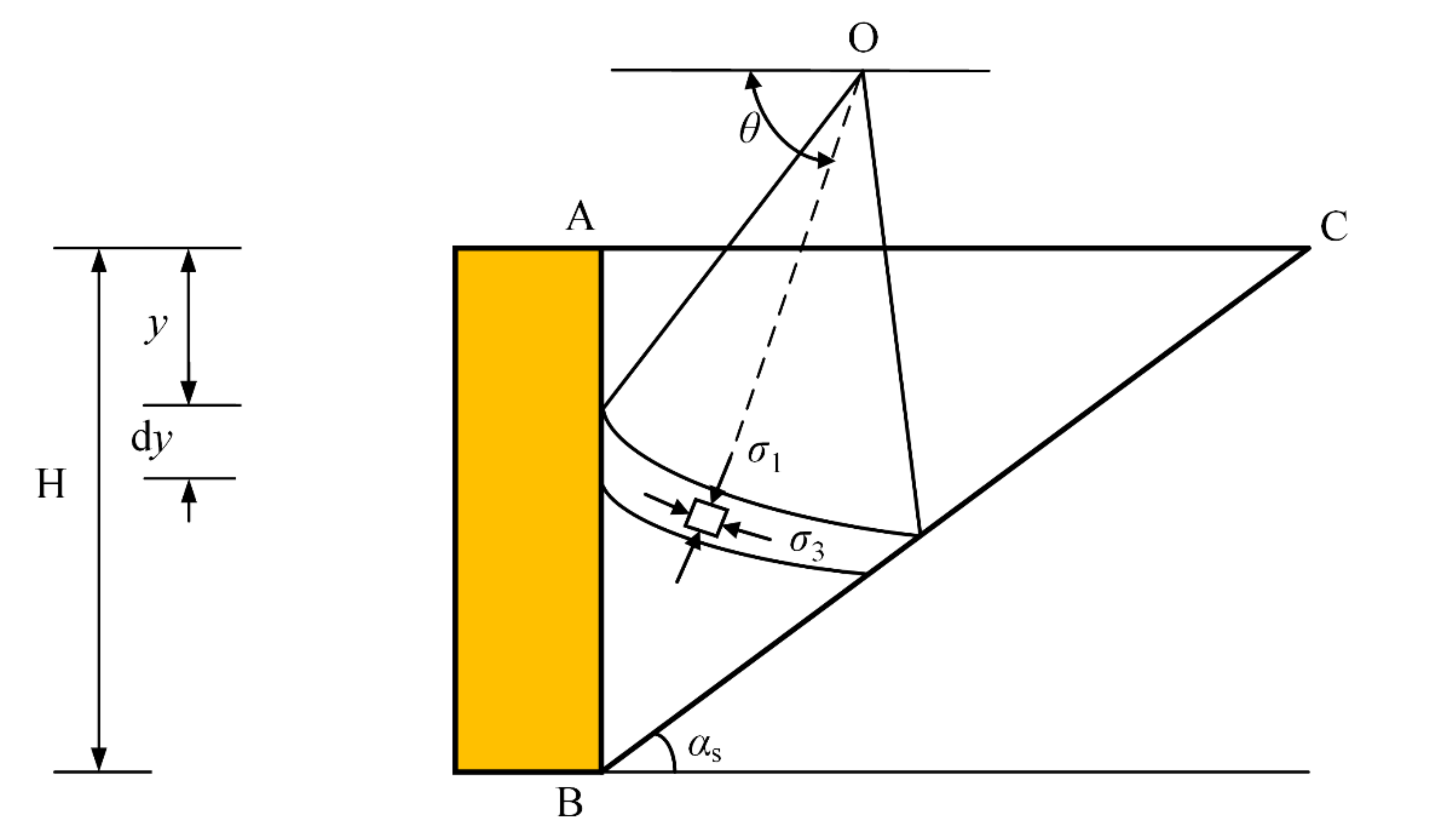
4.1. Method of Determining Potential Slip Planes

As shown in Figure 1, the retaining wall height is H, and the slip angle is ${\alpha }_s$.

In practice, the rotation angle of walls in RB is very small, which makes it extremely unlikely that the horizontal displacement of the backfill will reach the critical displacement, resulting in most of the soil behind the wall remaining in a nonlimiting state [19]. However, the basic assumption based on Coulomb’s earth pressure theory is that the soil within the wall height reaches a fully active state, that is, the shear strength of the soil behind the wall is fully developed. The concept of a quasi-slip cracking surface comes into play when the shear strength of the soil behind the wall is partially developed, assuming that a quasi-slip cracking surface appears behind the wall when the soil behind the wall has not reached a fully active state, and the angle between the quasi-slip cracking surface and the horizontal plane is the quasi-slip cracking angle.

The studies [36,37,38] revealed that interface friction angle is less than the soil friction angle and has little effect on the slip angle. Moreover, tests [5,7] show that the sliding surface essentially obeys Rankine’s theory.

When the retaining wall rotates, the inclination of the wall back is negligible, which is only suitable for vertical wall back. Therefore, the slip plane angle in Rankine’s formula is introduced as a quasi-slip crack angle for simplicity of calculation:

$${\alpha }_s={45}^{\circ }+\frac{\phi }{2}$$

(5)

where $\phi$ is soil friction angle, and ${\alpha }_s$ is crack angle.

4.2. Definition of Small Principal Stress Traces Parameters

4.2.1. Definition of Deflection Angle of Principal Stress

The soil wedge ABC behind the wall has three boundaries. AB represents the wall back, BC represents the sliding surface of soil mass, and AC represents the top surface of fill. It is assumed that the principal stress trace intersects with the wall back and sliding surface at points D and E, respectively. As illustrated in Figure 2a, assuming that the included angle between the direction of small principal stress and the vertical direction is ${\theta }_a$ at the wall–soil contact, Equations (6) and (7) can be obtained from the static equilibrium condition.

$${\sigma }_{1m}={\sigma }_1^a{\cos }^2{\theta }_a+{\sigma }_3^a{\sin }^2{\theta }_a$$

(6)

$${\tau }_{1m}=({\sigma }_1^a-{\sigma }_3^a)\sin {\theta }_a\cos {\theta }_a$$

(7)

where ${\sigma }_{1m}$ = normal stress at the wall–soil contact surface; ${\tau }_{1m}$ = shear stress in the soil at the wall–soil contact; ${\sigma }_1^a$ = maximum principal stress at the wall–soil contact surface; and ${\sigma }_3^a$ = minimum principal stress at the wall–soil contact surface. In addition, ${\theta }_a$ is the deflection angle of small principal stress.

The stresses at the wall–soil contact are subject to the Mohr–Coulomb criteria, which can be expressed as

$$N=\frac{{\sigma }_1^a}{{\sigma }_3^a}={\tan }^2({45}^{\circ }+\frac{\phi }{2})$$

(8)

$${\tau }_{1m}={\sigma }_{1m}\tan {\delta }_m$$

(9)

where N is the ratio of maximum principal stress to minimum principal stress, $\phi$ is the soil friction angle, and ${\delta }_m$ is the developed value of interface friction angle.

By solving Equations (6)–(9), Equation (10) can be obtained as follows

$${\theta }_a=\arctan \left[\frac{(N-1)+\sqrt{{(N-1)}^2-4N{\tan }^2{\delta }_m}}{2\tan {\delta }_m}\right]$$

(10)

where ${\theta }_a$ is the included angle between the direction of small principal stress and the vertical direction at the wall–soil contact surface, and ${\delta }_m$ is the mobilized value of interface friction angle.

It is assumed that ${\theta }_b$ is the included angle between the direction of small principal stress and the vertical direction at the potential slip plane. Equations (11) and (12) can be established:

$${\sigma }_{2m}={\sigma }_1^b{\sin }^2({\theta }_b-{\alpha }_s)+{\sigma }_3^b{\cos }^2({\theta }_b-{\alpha }_s)$$

(11)

$${\tau }_{2m}=({\sigma }_1^b-{\sigma }_3^b)\sin ({\theta }_b-{\alpha }_s)\cos ({\theta }_b-{\alpha }_s)$$

(12)

where ${\sigma }_{2m}$ = normal stress at the potential slip plane; ${\tau }_{2m}$ = shear stress at the potential slip plane; ${\sigma }_1^b$ = maximum principal stress at the potential slip plane; ${\sigma }_3^b$ = minimum principal stress at the potential slip plane.

As with Equations (8) and (9), Equations (13) and (14) can be obtained in the same way:

$$N=\frac{{\sigma }_1^b}{{\sigma }_3^b}={\tan }^2({45}^{\circ }+\frac{\phi }{2})$$

(13)

$${\tau }_{2m}={\sigma }_{2m}\tan {\phi }_m$$

(14)

where N is the ratio of maximum principal stress to minimum principal stress, $\phi$ is the soil friction angle, and ${\phi }_m$ is the developed value of soil friction angle.

By solving Equations (11)–(14), Equation (15) can be obtained:

$${\theta }_b={\alpha }_s+\arctan \left[\frac{(N-1)+\sqrt{{(N-1)}^2-4N{\tan }^2{\phi }_m}}{2N\tan {\phi }_m}\right]$$

(15)

where ${\theta }_b$ is the included angle between the direction of small principal stress and the vertical direction at the potential slip plane, and ${\phi }_m$ is the developed value of soil’s friction.

Equations (10) and (15) suggest that ${\theta }_a$ and ${\theta }_b$ are exclusively connected to parameters $N,\delta ,\phi$ and are unrelated to the depth. However, the principal stress deflection angle ${\theta }_{}$ in the soil is not a constant along the principal stress trace, as shown in Figure 2a.

4.2.2. Definition of Arc Trace Radius

Principal stress traces typically take the form of parabolas, catenaries, circular arcs, and so on. However, the choice of principal stress traces has little effect on the analytical solution of earth pressure, so for calculation convenience, this paper utilized circular principal stress traces [15]. The method for determining $R_{DE}$ and $R_{D\prime E\prime }$ involves first connecting points D and E, drawing the middle vertical line of line DE, and finally drawing a vertical line through point D. This normal intersects the mid-pipeline at point O. The radius of the arc DE is represented by lines OD and OE. The radius $R_{D\prime E\prime }$ of arc $D\prime E\prime$ is determined using the method presented in Figure 2b.

Figure 2b depicts the geometric features of the minor principal stress trace, assuming that the minimal principal stress trace is a circular curve. The length of the arc at the upper interface of the unit is $l_{\stackrel{⏜}{DE}}$, the center of the circle is O, and the depth of burial at point D is y. Although the length of the straight line OD is $R_{DE}$, the length of line $O^{\prime }D$ is $R_{D\prime E\prime }$. ${\theta }_a$ and ${\theta }_b$ are the angles of OD and OE to the horizontal, and ${\theta }_1$ is the angle between the vertical and line DE, which can be derived from the geometric relationships in Figure 2b. The following can be derived from the angle relationship of $\Delta$ODE:

$$2\left({\theta }_a+\gamma \right)+{\theta }_b-{\theta }_a={180}^{\circ }$$

(16)

$${\theta }_1+\gamma ={90}^{\circ }$$

(17)

where $\gamma$ is the included angle between segment DE and the horizontal direction.

The simplification of Equations (16) and (17) yields

$${\theta }_1=\frac{{\theta }_a+{\theta }_b}{2}$$

(18)

The length of line DE, denoted as $l_{DE}$, can be determined from the geometry of $\Delta$DEB by using the sine theorem as follows:

$$\frac{H-y}{\angle DEB}=\frac{l_{DE}}{\angle DBE}$$

(19)

$$\angle DBE={90}^{\circ }-{\alpha }_s$$

(20)

$$\angle DEB={90}^{\circ }+{\alpha }_s-{\theta }_1$$

(21)

Substituting Equations (20) and (21) into Equation (19) to simplify it yields

$$l_{DE}=\frac{(H-y)\cos {\alpha }_s}{\cos ({\theta }_1-{\alpha }_s)}$$

(22)

Equation (22) incorporates the geometric relations in the $\Delta$ODE and $\Delta$OD’E’ to derive the magnitude of $R_{DE}$ and $R_{D\prime E\prime }$.

$$R_{DE}=\frac{\frac{1}{2}{l}_{DE}}{\sin (\frac{{\theta }_b-{\theta }_a}{2})}=\frac{(H-y)a_2}{2}$$

(23)

$$R_{D\prime E\prime }=\frac{\frac{1}{2}{l}_{D\prime E\prime }}{\sin (\frac{{\theta }_b-{\theta }_a}{2})}=\frac{(H-y-dy)a_2}{2}$$

(24)

$$a_2=\frac{\cos {\alpha }_s}{\sin (\frac{{\theta }_b-{\theta }_a}{2})\cos ({\theta }_1-{\alpha }_s)}$$

(25)

where H is the retaining wall height, y is the depth of burial at point D, and dy is the length of line DD’.

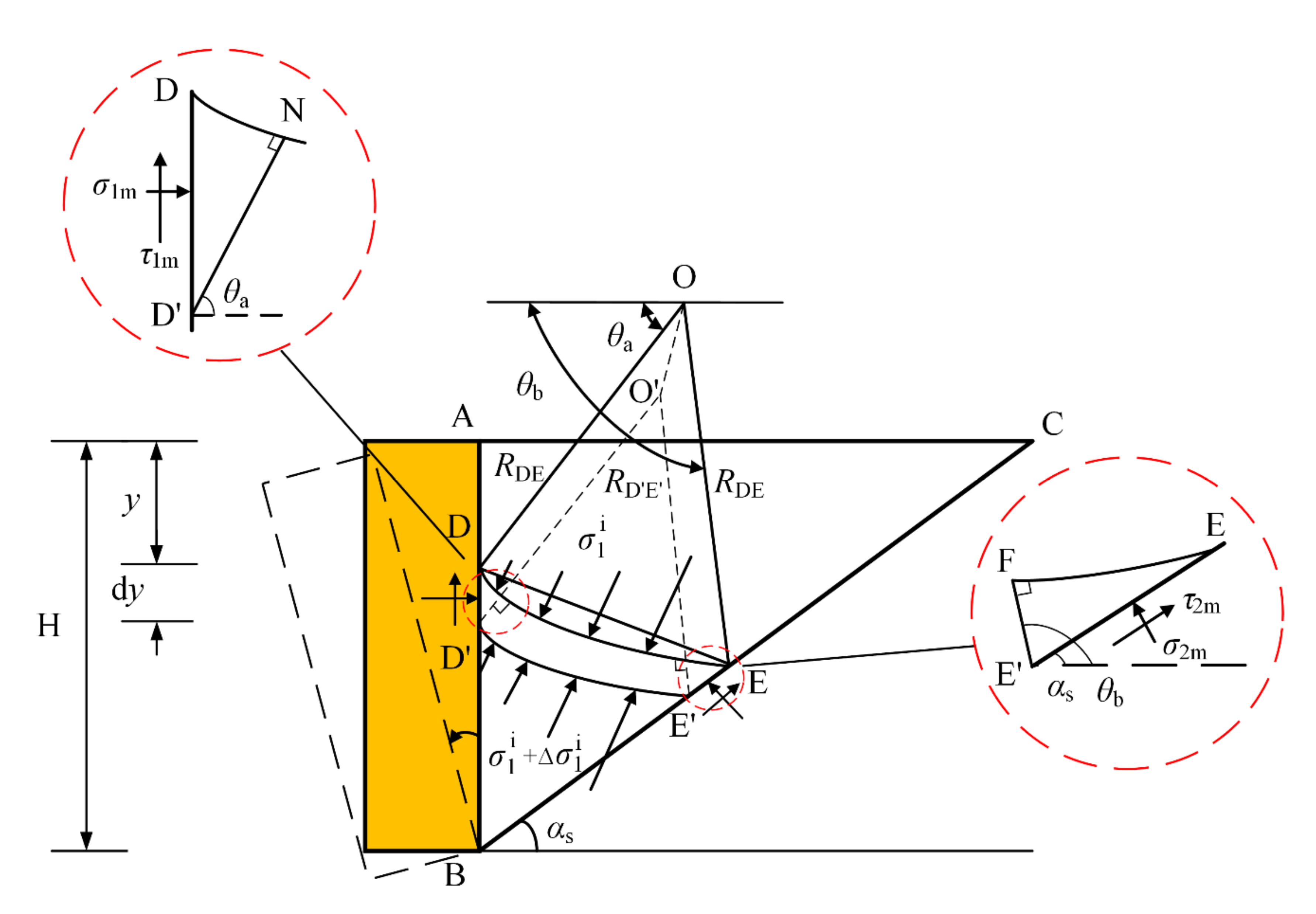
4.3. Analysis of Unit Forces at Wall–Soil Contact Surfaces and Potential Slip Crack Surfaces

Triangular elements are utilized for the wall–soil contact surface and soil slip crack surface, as shown in Figure 3. At the wall–soil contact and potential slip-cracking surfaces, the horizontal and vertical pressures ($F_x^{DD\prime }$, $F_y^{DD\prime }$, $F_x^{EE\prime }$, $F_y^{EE\prime }$) acting on the thin layer unit may can described as

$$F_x^{DD\prime }=l_{DD\prime }{\sigma }_{1m}$$

(26)

$$F_y^{DD\prime }=l_{DD\prime }{\tau }_{1m}$$

(27)

$$F_x^{EE\prime }=({\tau }_{2m}\cos {\alpha }_s-{\sigma }_{2m}\sin {\alpha }_s)l_{EE\prime }$$

(28)

$$F_y^{EE\prime }=({\tau }_{2m}\sin {\alpha }_s+{\sigma }_{2m}\cos {\alpha }_s)l_{EE\prime }$$

(29)

where $l_{DD\prime }$ and $l_{EE\prime }$ are the lengths of the unit at the wall–soil contact surface $DD\prime$ and potential slip plane $EE\prime$ of the soil, respectively, which can be solved in Figure 3 through the geometric relationship of Δ DD’N and Δ EE’F: $l_{D\prime N}$ = $l_{E\prime F}$.

$$\left\{\begin{array}{l}{l}_{DD\prime }=dy\\ l_{EE\prime }=\frac{dy\sin {\theta }_a}{\cos ({\theta }_b-{\alpha }_s)}\end{array}\right.$$

(30)

4.4. Analysis of the Upper and Lower Interfaces of Thin-Layer Units

It is assumed that the maximum principal stress at point D of the soil at the wall–soil contact is ${\sigma }_1^a$. The major principal stress at the parting level is considered to vary linearly with depth, as depicted in Figure 3. The maximum principal stress at an arbitrary point i on the upper interface of a bending thin-layer cell can be given as

$${\sigma }_1^i={\sigma }_1^a+\gamma R_{DE}\left(\sin \theta -\sin {\theta }_a\right)$$

(31)

where $\gamma$ is the gravity of soil. $\theta$ is the angle between the line connecting point i and the center of its circular arc and the horizontal line, and ${\theta }_a$ is the angle between the line connecting point D and the center of the circle and horizontal direction. The horizontal force $F_x{}^{DE}$ and vertical force $F_y{}^{DE}$ acting on the top interface DE from the wall–soil contact to the potential slip-cracking surface of the soil may be represented as

$$F_x^{DE}={\displaystyle {\int }_{{\theta }_{{}_a}}^{{\theta }_{{}_b}}{\sigma }_1^i}{R}_{DE}\cos \theta d\theta$$

(32)

$$F_y^{DE}={\displaystyle {\int }_{{\theta }_a}^{{\theta }_{\mathrm{b}}}{\sigma }_1^i}{R}_{DE}\sin \theta d\theta$$

(33)

Substituting Equation (31) into Equations (32) and (33) yields

$$F_x^{DE}={\sigma }_1^a{R}_{DE}{b}_1+\frac{1}{2}\gamma R_{DE}^2{b}_1^2$$

(34)

$$F_y^{DE}={\sigma }_1^a{R}_{DE}{b}_2+\gamma R_{DE}^2{b}_3$$

(35)

where

$$b_1=\sin {\theta }_b-\sin {\theta }_a$$

(36)

$$b_2=\cos {\theta }_a-\cos {\theta }_b$$

(37)

$$b_3=\frac{{\theta }_b-{\theta }_a}{2}-\frac{\sin 2{\theta }_b-\sin 2{\theta }_a}{4}-\sin {\theta }_a{b}_2$$

(38)

The horizontal force $F_x{}^{D\prime E\prime }$ and vertical force $F_y{}^{D\prime E\prime }$ on the lower interface of the differential unit $D\prime E\prime$ may be calculated in the same way as the forces acting on DE at the higher interface of the differential unit.

$$F_x^{D\prime E\prime }=({\sigma }_1^a+\Delta {\sigma }_1^a)R_{D\prime E\prime }{b}_1+\frac{1}{2}\gamma R_{D\prime E\prime }^2{b}_1^2$$

(39)

$$F_y^{D\prime E\prime }=({\sigma }_1^a+\Delta {\sigma }_1^a)R_{D\prime E\prime }{b}_2+\gamma R_{D\prime E\prime }^2{b}_3$$

(40)

where $\Delta {\sigma }_1^a$ is the stress increment relative to point D. Moreover, $F_x{}^{D\prime E\prime }$ and $F_y{}^{D\prime E\prime }$ are the horizontal force and vertical force of the differential unit $D\prime E\prime$, respectively.

4.5. Thin-Layer Cell Gravity Analysis

The curved-edge lamellar unit, after expansion, can be considered a trapezoid. Accordingly, the gravity of a curved-edge thin layer is calculated as follows:

$$dA=\frac{\gamma (l_{\stackrel{⏜}{DE}}+l_{\stackrel{⏜}{D\prime E\prime }})t}{2}$$

(41)

where $\gamma$ is the density of the backfill soil; dA is the gravity of the curved-edge thin layer; t is the height of the thin-layered cell; and $l_{\stackrel{⏜}{DE}}$ and $l_{\stackrel{⏜}{D\prime E\prime }}$ are the arc length of the upper and lower boundary of the element, respectively, which can be expressed as

$$l_{\stackrel{⏜}{DE}}=\frac{({\theta }_b-{\theta }_a)(H-y)a_2}{2}$$

(42)

$$l_{\stackrel{⏜}{D\prime E\prime }}=\frac{({\theta }_b-{\theta }_a)(H-y-dy)a_2}{2}$$

(43)

t is the height of the thin-layered cell, which can be expressed according to the geometry shown in Figure 3.

$$t=l_{\stackrel{⏜}{D\prime N}}=\sin {\theta }_{a}dy$$

(44)

$l_{\stackrel{⏜}{D\prime N}}$ is the arc length of D’N. ${\theta }_a$ is the included angle between the direction of small principal stress and the vertical direction at the wall–soil contact surface.

4.6. Equilibrium Control Equation for Thin Layer Cells

The equilibrium control equation can be obtained from the static equilibrium condition of the thin-layer unit, which can be expressed as

$$F_x^{DD\prime }-F_x^{DE}+F_x^{D\prime E\prime }+F_x^{EE\prime }=0$$

(45)

$$F_y^{DD\prime }-F_y^{DE}+F_y^{D\prime E\prime }+F_y^{EE\prime }-dA=0$$

(46)

The forces applied to the unit are then substituted into Equations (45) and (46) to simplify them and obtain the controlling equation for the circularly curved thin layer unit as follows:

$$\begin{array}{l}{a}_1{\sigma }_{1m}dy-\frac{a_2{a}_3}{2}{\sigma }_1^{a}dy+\frac{a_2{a}_3}{2}(H-y-\frac{dy}{2})d{\sigma }_1^a-\frac{\gamma a_2^2{a}_4}{2}(H-y)\\ -\frac{a_5\gamma dy}{2}(H-y-\frac{dy}{2})=0\end{array}$$

(47)

where

$$a_1=(\tan \phi -\tan {\alpha }_s)\tan \delta -(1+\tan \phi \tan {\alpha }_s)$$

(48)

$$a_2=\frac{\cos {\alpha }_s}{\cos ({\theta }_1-{\alpha }_s)\cdot \sin (\frac{{\theta }_b-{\theta }_a}{2})}$$

(49)

$$a_3=b_2(\tan \phi -\tan {\alpha }_s)-b_1(1+\tan \phi \tan {\alpha }_s)$$

(50)

$$a_4=\frac{b_1^2}{2}(1+\tan \phi \tan {\alpha }_s)+b_3(\tan \phi -\tan {\alpha }_s)$$

(51)

$$a_5=a_2\sin {\theta }_a({\theta }_b-{\theta }_a)(\tan \phi -\tan {\alpha }_s)$$

(52)

Equation (47) consists of two unknowns, ${\sigma }_{1\mathrm{m}}$ and ${\sigma }_1^a$, which are determined using Equation (6).

$${\sigma }_{1\mathrm{m}}=a_6{\sigma }_1^a$$

(53)

where

$$a_6={\cos }^2{\theta }_a+\frac{{\sin }^2{\theta }_a}{N}$$

(54)

By substituting Equations (53) and (54) into Equation (47), a differential equation for the major principal stress ${\sigma }_1^a$ can be obtained.

$$\frac{\mathrm{d}{\sigma }_1^a}{dy}-\frac{f_1}{H-y}{\sigma }_1^a-\frac{\gamma }{f_2}=0$$

(55)

where

$$f_1=1-\frac{2a_1{a}_6}{a_2{a}_3}$$

(56)

$$f_2=\frac{a_2{a}_3}{a_2^2{a}_4+a_5}$$

(57)

Solving differentiated Equation (55) yields

$${\sigma }_1^a=C{(y-H)}^{-f_1}+\frac{\gamma (y-H)}{(1+f_1)f_2}$$

(58)

$${\sigma }_{1m}=a_{6}C{(y-H)}^{-f_1}+\frac{a_6\gamma (y-H)}{(1+f_1)f_2}$$

(59)

where C is a constant to be determined. According to the boundary condition, ${\sigma }_{1\mathrm{m}}=0$ at y = 0, C can be solved.

$$C=-\frac{\gamma {(-H)}^{1+f_1}}{(1+f_1)f_2}$$

(60)

The active earth pressure strength ${\sigma }_{1\mathrm{m}}$ can be calculated by substituting Equation (60) into (59), which yields

$${\sigma }_{1m}=K\gamma \left[H{(1-\frac{y}{H})}^{-f_1}+(y-H)\right]$$

(61)

where

$$K=\frac{a_6}{(1+f_1)f_2}$$

(62)

Equation (61) is the formula for the active earth pressure derived in this study.

The combined active earth pressure force $E_a$ on the retaining wall can be described as

$$E_a={\displaystyle {\int }_0^H{\sigma }_{1m}}dy$$

(63)

The active earth pressure bending moment $M$ of the retaining wall can be expressed as

$$M={\displaystyle {\int }_0^H{\sigma }_{1m}(H-y)}dy$$

(64)

The point of application of the resultant force on the retaining wall is $h_p$.

$$h_p=\frac{M}{E_a}=\frac{2(1-f_1)}{3(2-f_1)}H$$

(65)

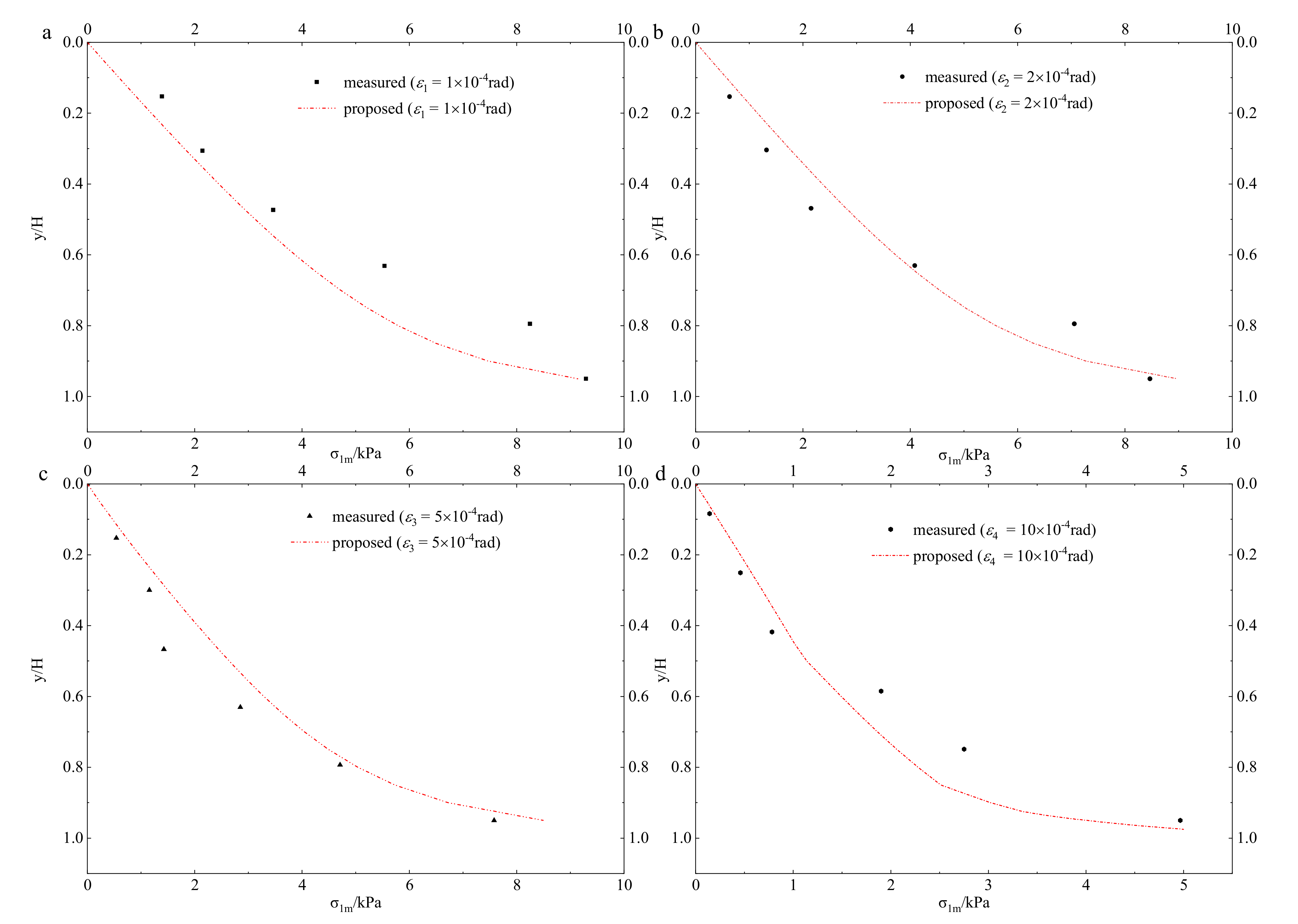
5. Verification by Comparison

A model test (Figure 4a–c) was conducted by Fang et al. [19], simulating sandy soil under semi-infinite conditions. The model test parameters were wall height H = 1.0 m, soil weight $\gamma =15.34{\mathrm{kN}/\mathrm{m}}^3$, soil friction angle $\phi ={33.4}^{\circ }$, interface friction angle $\delta =2/3\phi$, and void ratio $e=0.706$. The experimental values were compared for three different wall rotations of ε₁, ε₂, or ε₃. Figure 4d shows the experimental soil pressure values obtained by Simita et al. [15] for a retaining wall with sand backfill soil behind the wall in RB obtained via model box experiments. The test parameters included wall height H = 0.6 m, soil weight $\gamma =15.92{\mathrm{k} \mathrm{N}/\mathrm{m}}^3$, soil friction angle $\phi ={36}^{\circ }$, interface friction angle $\delta ={22}^{\circ }$, void ratio $e_{max}=0.740$ and $e_{\min }=0.500$, relative density of the soil $D_r=45\%$, and wall rotation ${\epsilon }_4=10\times {10}^{-4}$ rad.

The soil along the wall height is in a nonlimiting state from Fang’s data when the wall rotation angle is ε₁, ε₂, or ε₃ by calculating the soil displacement Sz along wall depth. It can be observed in Figure 4a–c that from the surface to a depth of 0.5 m, the earth pressure distribution curve was linear. At depths greater than 0.5 m, the earth pressure distribution curve exhibited clear nonlinearity and a tendency to diverge outwards. As the depth increased (from the wall top), the rate of increasing earth pressure increased. The results of the theoretical approach used in this paper were in good agreement with Fang’s [19] experimental values. When the wall rotation was ε₄, the upper half of the soil in the height of the wall was in ultimate equilibrium, whereas the lower half part of the soil remained in a nonlimiting state. Figure 4d compares the theoretical estimated values from this research against Smita’s experimental data [15]. In Figure 4d, unlike in Figure 4a–c, an inflection point in the earth pressure distribution curve was observed at a depth of 0.5 m because of the transition from a nonlimiting state to an active limit state of the soil behind the wall in this area. The theoretical method presented in this study is corroborated by Smita’s experimental data [15], and the earth pressure distribution curve exhibited an inflection point.

6. Parameter Sensitivity Analysis

Because the influence of the rotation angle ε and interface friction angle on the soil pressure distribution and resultant force is the focus of the present study, a parametric sensitivity analysis was conducted to explore their effects on the research content. The retaining wall height H = 1m, soil weight $\gamma =15.34\mathrm{kN}/{\mathrm{m}}^3$, soil friction angle $\phi =33.4°$, wall–soil angle $\delta =2/3\phi$, and void ratio $e=0.706$. Other values were assumed for assessing the effects of other relevant factors.

6.1. Analysis of the Effect of the Rotation Angle ε of the Retaining Wall on the Earth Pressure Distribution

It was assumed that the x-axis represents the σ1 m axis and the y-axis represents the y/H axis in Figure 5. As shown in Figure 5, the earth pressure strength distribution tended to retreat in the negative direction of the x-axis with increasing rotation angle. According to the traditional earth pressure theory [1,2], when the retaining wall rotates outwards about the base from its resting condition, the earth pressure starts to decrease below the static earth pressure. As the rotational angle ε increased from 0 to 5 × 10⁻⁴ rad, the earth pressure distribution curve inclined via translation toward the negative direction of the x-axis while maintaining a linear and consistent outward divergence. This was attributed to the soil along the wall height being in a nonlimiting state and the shear strength not being fully developed before the wall rotation increased to 5 × 10⁻⁴ rad. This results in insufficient friction between the wall and soil, and the soil’s and interface friction angle at the bottom of the wall being minimal and causing the soil pressure distribution curve to diverge as the depth increased. The earth pressure distribution curve exhibited an inflection point as the rotation angle increased from 5 × 10⁻⁴ rad to 100 × 10⁻⁴ rad, and the inflection point moved upwards as the angle increased. The curve above the inflection point appeared as a retracted convex curve, whereas the curve below the inflection point exhibited a concave curvature that diverges outward.

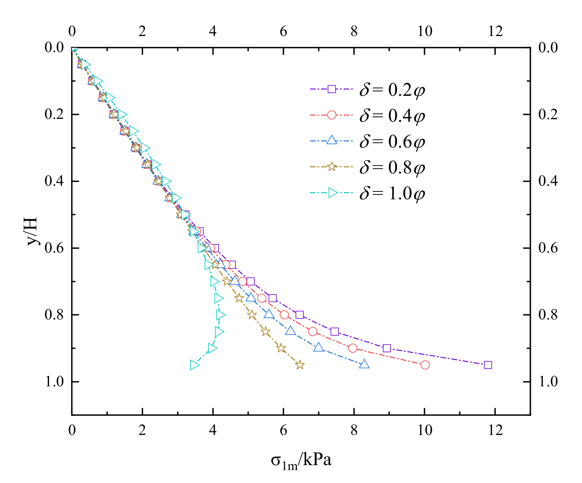
6.2. Analysis of the Effect of Interface Friction Angle δ on the Earth Pressure Distribution

An angle of rotation of 1 × 10⁻⁴ rad in the wall was considered for the analysis for $\delta =0.2\phi$ to $\phi$.

As can be observed in Figure 6, the soil pressure distribution curve in the upper half of the soil mass was linear as $\delta$ changed. A further increase in $\delta$ resulted in the curve in the lower half of the soil shifting toward the negative direction of the x-axis. For the same soil depth, the earth pressure did not vary significantly in the upper half of the soil as the depth increased, but it decreased sharply in the lower half of the soil as $\delta$ increased. Moreover, the decrease in earth pressure became more pronounced as the soil depth increased. This observation can be explained by the fact that, in RB mode, the fill behind the wall has a tendency to slide downwards relative to the retaining wall. Further, when the friction angle between the wall and the soil is considered, the wall surface will exert an upward frictional force on the fill to prevent it from sliding downward, resulting in a deflection in the principal stresses and the soil arch effect. This friction exerts an upward restraining force on the soil, counteracting the gravity of the fill to some extent and lowering the soil weight. Thus, the earth pressure in the soil decreases as $\delta$ increases.

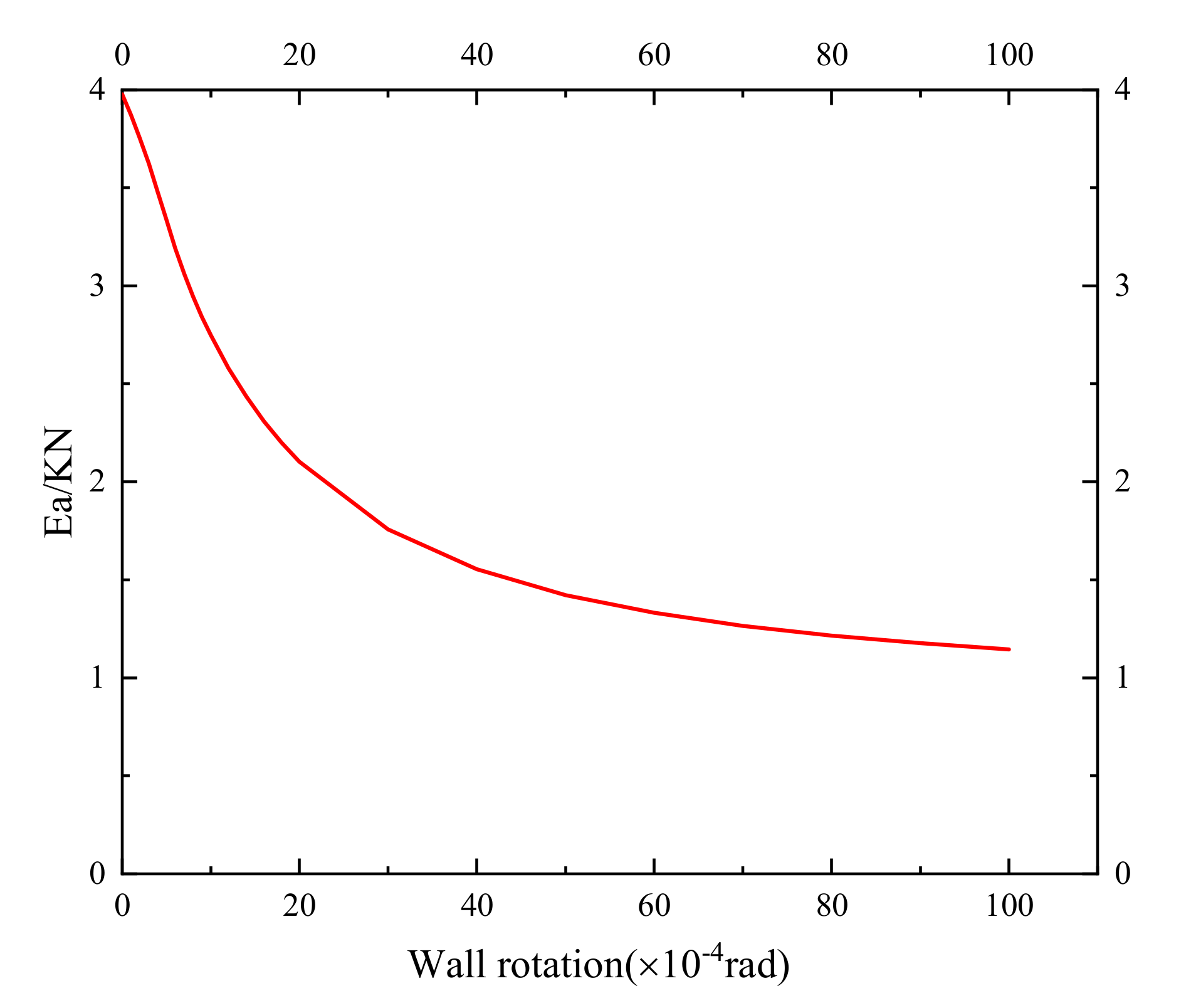
6.3. Effect of Rotation Angle on Resultant Forces

When the rotation angle was zero, the wall was at rest, as shown in Figure 7. The resultant force dropped sharply once the rigid wall began rotating. With the wall rotation increasing to approximately 20 × 10⁻⁴ rad, the rate of reduction of the combined force slowed until the magnitude of the resultant force stabilized at approximately 100 × 10⁻⁴ rad. In this case, the rise in angle had a smaller effect on the combined earth pressure because, at larger angles, most of the soil displacement behind the wall reached a critical value and the shear strength was fully developed.

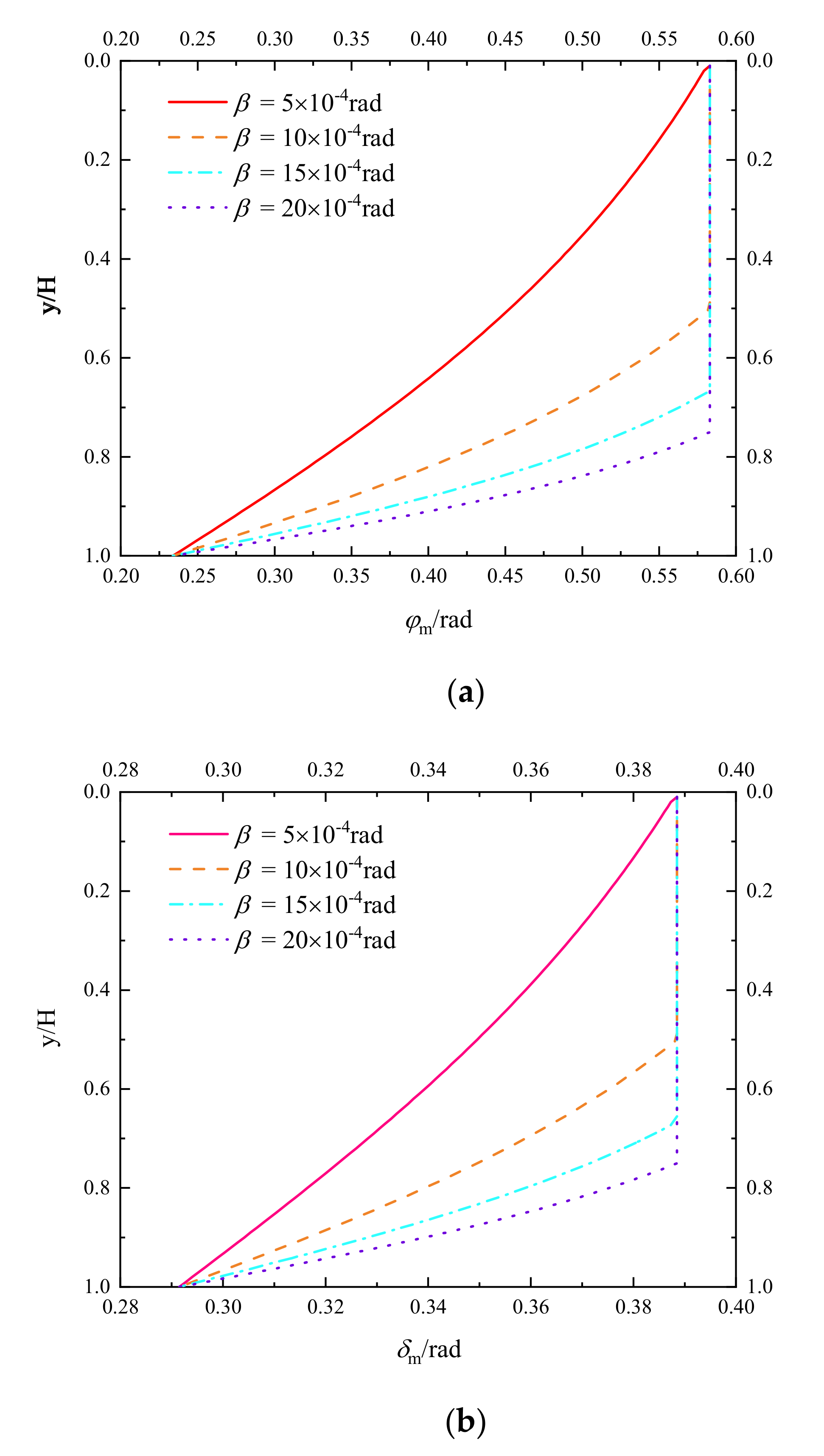
6.4. Friction Angle Effctive Values at Different Angles of Rotation

It can be inferred from Figure 8 that as the altitude of soil mass increased, the effective value of the friction angle increased and it exhibited a nonlinear relationship with depth. Until that soil reached its active limit, the friction angle was fully developed and its magnitude was a constant. As the angle of rotation increased, the height at which the friction angle reached a constant value decreased. The height at which the soil friction angle reached a constant value decreased by approximately 1/2H as the angle of rotation increased from 5 × 10⁻⁴ rad to 10 × 10⁻⁴ rad, the height at which the soil friction angle reached a constant value decreased by approximately 1/4H as the angle increased from 10 × 10⁻⁴ rad to 15 × 10⁻⁴ rad, and the height at which the soil friction angle reached a constant value decreased by approximately 1/8H as the angle increased from 15 × 10⁻⁴ rad to 20 × 10⁻⁴ rad. Evidently, the larger the angle of rotation, the sooner the soil friction angle reached a constant value.

7. Conclusions

(1)

The primary stress traces in RB of retaining walls were utilized for calculating earth pressure in this study. The effect of the soil arch effect on the deflection of the principal stresses was considered, and a curved thin-layer cell method was employed to characterize the inhomogeneity of the stress distribution at the interface above and below the cell. A rigorous theoretical derivation was also performed.

(2)

The notion of friction angle developed value was leveraged in this study to develop a nonlinear relationship between the mobilized value of the friction angle and horizontal displacement of the soil to characterize the stress state of the soil behind the wall under nonlimiting situations. Parametric analysis indicated that the closer the soil was to the top of the wall, the higher the friction angle developed value, provided that the wall rotation was a constant.

(3)

The analytical solution of the soil pressure strength derived in this paper was compared with the model test data for validation, and the agreement was good. This verified the rationality of the proposed theory. The active earth pressure strength increased monotonically with depth within the wall height in RB. The earth pressure intensity exhibited a linear variation in the upper half of the soil but a stronger nonlinear distribution in the lower half.

(4)

The earth pressure intensity distribution decreased as the angle of rotation increased, as revealed in parameter sensitivity experiments. Upon reaching a certain angle of rotation, an inflection point in the earth pressure intensity distribution curve was observed due to the upper soil reaching ultimate equilibrium while the lower soil remained in a nonlimiting state. If the rotation angle was fixed, the horizontal earth pressure strength increased and then decreased as the interface friction angle increased.

(5)

Engineers can use the monitoring data of the retaining wall to judge the displacement mode of the retaining wall and select a reasonable calculation method.

(6)

This paper on can provide a reference for soil pressure calculation for rotating walls, but the study had some limitations. First of all, it was assumed that the fill behind the wall was of the same nature, without consideration of layering according to soil properties. Secondly, the study was only for the condition of sandy soil. Further research is needed on the earth pressure of rotating walls with cohesive fill soils. Last but not least, reinforced walls and geosynthetics are always used in practical projects. We will study this field in depth in the follow-up work.

References

1. Coulomb, C.A. Essai sur une Application des Règles de Maximis et Minimis Aquelques Problèmes de Statique, Relatifs a l’Architecture; Imprimerie Royale: Paris, France, 1776. (In French) [Google Scholar]
2. Rankine, W. On the stability of loose earth. Philos. Trans. R. Soc. Lond. 1857, 147, 9–27. [Google Scholar]
3. Terzaghi, K. Theoretical Soil Mechanics; Wiley: New York, NY, USA, 1943; pp. 40–43. [Google Scholar]
4. Kingsley, H.W. Geostatic wall pressures. Geotech. Eng. 1989, 115, 1321–1325. [Google Scholar]
5. Tsagareli, Z. Experimental investigation of the pressure of a loose medium on re-taining walls with a vertical back face and horizontal backfill surface. Soil Mech. Found. Eng. 1965, 2, 197–200. [Google Scholar] [CrossRef]
6. James, R.; Bransby, P. Experimental and theoretical investigations of a passivepressure problem. Geotechnique 1970, 20, 17–37. [Google Scholar] [CrossRef]
7. Matsuo, M.; Kenmochi, S.; Yagi, H. Experimental study of retaining wall by field tests. Soils Found. 1978, 18, 27–41. [Google Scholar] [CrossRef]
8. Tang, Z. A rigid retaining wall centrifuge model test of cohesive soil. ChongqingJiaotong Univ. 1988, 25, 48–56. [Google Scholar]
9. Yang, M.; Dai, X.; Zhao, M.; Luo, H. Experimental study on active earth pressure of cohesionless soil with limited width behind retaining wall. Chin. J. Geotech. Eng. 2016, 38, 131–137. (In Chinese) [Google Scholar]
10. Dou, G.; Xia, J.; Yu, W.; Yuan, F.; Bai, W. Non-limit passive soil pressure on rigid retaining walls. Int. J. Min. Sci. Technol. 2017, 27, 581–587. [Google Scholar] [CrossRef]
11. Yang, T.; He, H.J. Calculation of unlimited passive earth pressure in the model of RBT movement. Adv. Mater. Res. 2011, 250–253, 1572–1577. [Google Scholar] [CrossRef]
12. Wang, S.; Cheng, Y. Determination of active earth pressure behind retaining wall rotating about wall toe. Rock Soil Mech. 2011, 32, 2139–2145. (In Chinese) [Google Scholar]
13. Li, D.; Wang, W.; Zhang, Q. Lateral Earth Pressure behind Walls Rotating about Base considering Arching Effects. Math. Probl. Eng. 2014, 2014, 715891. [Google Scholar] [CrossRef]
14. Cao, W.; Zhang, H.; Liu, T.; Tan, X. Analytical solution for the active earth pressure of cohesionless soil behind an inclined retaining wall based on the curved thin-layer element method. Comput. Geotech. 2020, 128, 103851. [Google Scholar] [CrossRef]
15. Smita, P.; Kousik, D. Study of Active Earth Pressure behind a Vertical Retaining Wall Subjected to Rotation about the Base. Int. J. Geomech. 2020, 20, 04020028. [Google Scholar]
16. Conte, E.; Troncone, A.; Vena, M. A method for the design of embedded cantilever retaining walls under static and seismic loading. Geotechnique 2017, 67, 1081–1089. [Google Scholar] [CrossRef]
17. Jayatheja, M.; Anasua, G.R. Earth Pressures on Retaining Walls backfilled with Red Soil admixed with Building Derived Materials under Rotational Failure mode. Geomech. Geoengin. 2021, 1912409. [Google Scholar] [CrossRef]
18. Fathipour, H.; Payan, M.; Chenari, R.J. Limit analysis of lateral earth pressure on geosynthetic- reinforced retaining structures using finite element and second-order cone programming. Comput. Geotech. 2021, 134, 104119. [Google Scholar] [CrossRef]
19. Fang, Y.; Isao, I. Static earth pressures with various wall movements. Geotech. Eng. 1986, 112, 317–333. [Google Scholar] [CrossRef]
20. Wang, S.C.; Sun, B.J.; Shao, Y. Modified Computational Method for Active earth pressure. Rock Soil Mech. 2015, 36, 1375–1379. (In Chinese) [Google Scholar]
21. Xie, T.; Luo, Q.; Zhang, L. Relationship between earth pressure and wall displacement based on Coulomb Earth pressure model. Chin. J. Geotech. Eng. 2018, 40, 194–200. (In Chinese) [Google Scholar]
22. Chen, L. Active earth pressure of retaining wall considering wall movement. Eur. J. Environ. Civ. Eng. 2014, 18, 910–926. [Google Scholar] [CrossRef]
23. Xu, R.Q.; Liao, B.; Wu, J. Computational Method for active earth pressure of cohensive soil under non-limit state. Rock Soil Mech. 2013, 34, 148–154. [Google Scholar]
24. Keshvarz, A.; Ebrahimi, M. The effects of the soil-wall adhesion and friction angle on the active lateral earth pressure of circular Retaining walls. Int. J. Civ. Eng. 2016, 14, 97–105. [Google Scholar] [CrossRef]
25. Chang, M. Lateral earth pressures behind rotating walls. Can. Geotech. J. 1997, 34, 498–509. [Google Scholar] [CrossRef]
26. Gong, C.; Yu, J.; Xu, R.; Wei, G. Calculation of earth pressure against rigid retaining wall rotating outward about base. J. Zhejiang Univ. Eng. Sci. 2005, 39, 1690–1694. (In Chinese) [Google Scholar]
27. Sangchul, B. Active earth pressure behind retaining walls. Geotech. Eng. 1985, 111, 407–412. [Google Scholar]
28. Niedostatkiewicz, M.; Lesniewska, D.; Jacek, T. Experimental Analysis of Shear Zone Patterns in Cohesionless for Earth Pressure Problems Using Particle Image Velocimetry. Strain 2011, 47, 218–231. [Google Scholar] [CrossRef]
29. Bourgeois, E.; Soyez, L.; Kouby, A.L. Experimental and numerical study of the behavior of a reinforced-earth wall subjected to a local load. Comput. Geotech. 2011, 38, 515–525. [Google Scholar]
30. Hu, J.Q.; Zhang, Y.X.; Chen, L. Study on active earth pressure on retaining wall in non-limit state. Chin. J. Geotech. Eng. 2013, 35, 381–387. (In Chinese) [Google Scholar]
31. Sherif, M.; Fang, Y.; Sherif, R.I. Ka and Ko behind rotating and non-yielding walls. Geotech. Eng. 1984, 110, 41–56. [Google Scholar] [CrossRef]
32. Xu, R.Q. Methods of earth pressure calculation for excavation. J. Zhejiang Univ. Eng. Sci. 2000, 34, 370–375. (In Chinese) [Google Scholar]
33. Matsuzawa, H.; Hararika, H. Analyses of active earth pressure against rigid retaining walls subjected to different modes of movement. Soils Found. 1996, 36, 51–65. [Google Scholar] [CrossRef]
34. Naikai, T. Finite element computations for active and passive earth pressure probems of retaining wall. Soils Found. 1985, 25, 98–112. [Google Scholar] [CrossRef]
35. Li, G.; Zhang, B.; Yu, Y.Z. Soil Mechanics, 2nd ed.; Tsinghua University Press: Beijing, China, 2013; p. 223. ISBN 978-7-302-33176-6. (In Chinese) [Google Scholar]
36. Sanjay, K.S. Dynamic active thrust from c–φ soil backfills. Soil Dyn. Earthq. Eng. 2011, 31, 526–529. [Google Scholar]
37. Zhou, Y.T. Active earth pressure against rigid retaining wall considering effects of wall–soil friction and inclinations. KSCEJ. Civ. Eng. 2018, 22, 4901–4908. [Google Scholar] [CrossRef]
38. Liu, H.; Kong, D.Z. Active Earth Pressure of Finite Width Soil Considering Intermediate Principal Stress and Soil Arching Effects. Int. J. Geomech. 2022, 22, 04021294. [Google Scholar] [CrossRef]
Figure 2. (a) Definition of small principal stress traces parameters. (b) Definition of arc trace radius.
Applsci 12 09638 g002
Figure 3. Force analysis of a curved thin-layer cell.
Applsci 12 09638 g003
Figure 4. Comparisons between existing theoretical solutions and experimental data with varying rotation angles: (a) ε1 = 1 × 10⁻⁴ rad of Fang; (b) ε2 = 2 × 10⁻⁴ rad of Fang; (c) ε3 = 5 × 10⁻⁴ rad of Fang [19]; (d) ε4 = 5 × 10⁻⁴ rad of Smita [15].
Applsci 12 09638 g004
Figure 5. Horizontal active earth pressure distribution along wall depth with varying rotation angle.
Applsci 12 09638 g005
Figure 6. Horizontal active earth pressure distribution along wall depth with varying interface friction angles δ.
Applsci 12 09638 g006
Figure 7. Combined earth pressure forces with varying rotation angles.
Applsci 12 09638 g007
Figure 8. Effect of rotation angles on the effective value distribution along wall depth of (a) soil friction angle φm and (b) interface friction angle δm.
Applsci 12 09638 g008