Constant Force Control of Centrifugal Pump Housing Robot Grinding Based on Pneumatic Servo System

Abstract

In order to solve the problem of constant force control in the robot grinding process of a centrifugal pump housing a circular inner surface, this study used the force–position hybrid control mode based on a pneumatic servo system to realize the constant control of grinding force. In this process, the manipulator realizes the position and pose control of the end grinding device, and the end grinding device realizes the constant force control in the grinding process. The mathematical model of the pneumatic system is established and linearized by using the gas balance state equation, the adiabatic equation of the isentropic process, and the Sanville flow equation. The balance equation of the cylinder piston was established by using Newton’s second law, the transfer function of the contact force between the grinding device and workpiece was obtained, and the stability of the pneumatic control system was determined by the Hurwitz criterion. The PID algorithm was used to improve the displacement response speed of the system and eliminate the impact and oscillation in the force response. The feasibility, stability, and robustness of the system were verified by simulation experiments. This method has the advantages of simple control, a small amount of calculation, and a fast response, as well as providing a feasible scheme for the popularization and application of robot grinding technology.

1. Introduction

Grinding and polishing technology is one of the most essential technologies for the final processing of free-form surface products, such as faucets, turbine blades, molds, wings, camshafts, crankshafts, and sculptures. However, the grinding and polishing process of these parts is predominantly manual at present, which is not only time-consuming but also has low efficiency, high labor costs, poor stability, and poor process consistency. At the same time, long-term manual grinding and polishing can also damage the health of operators [1]. In recent years, robot machining has attracted much attention because of its low cost, high flexibility, and strong ability to be integrated with actuators, sensors, and different end actuators [2]. As automatic equipment, robots have adequate flexibility and are more suitable for grinding and polishing free-form surfaces. Therefore, industrial robot machining has become an effective and economical solution to deal with complex parts [3]. In the process of robot grinding, the robot requires contact with the workpiece. Too much contact force between the end of the robot and the workpiece can damage the robot or workpiece. Too little contact force can lead to the workpiece not meeting the technical requirements, in addition to the insufficient accuracy of the contact between the workpiece and the grinding robot [4]. Therefore, the constant force and compliant motion control of grinding and polishing robots has become the main research direction for improving grinding and polishing quality [5].

Many scholars have explored the force control of grinding robots. Ting Wang et al. [4] designed a PID-IMC controller to realize the constant force control of robot grinding based on the principle of internal model control (IMC). Jinno M et al. [6] developed a robot grinding system and studied the method and direction of force application in the grinding process. Tahvilian AM et al. [7] developed a flexible tool-holder robot grinding system based on a semi-analytical grinding force model for grinding hard or brittle materials. Wang Fei et al. [8] proposed a fast translation detection strategy and fuzzy force control algorithm to realize the automatic grinding of the inner surface of a cavity by the robot. Adnan Jabbar Attiya et al. [9] proposed a robot grinding system with a flexible wrist, which uses a fuzzy PID controller to control the grinding force when grinding a propeller surface. A method based on the B-spline curve was proposed to optimize the robot’s grinding force in the grinding process [10]. Zhang T et al. [11] proposed a reinforcement learning force control algorithm based on the pressure release model, which is used to control robot constant force grinding. Zhou Pokuang et al. [12] proposed a self-adaptability control method based on the fuzzy PID algorithm to eliminate the residual texture and harmful stress concentration of the robot grinding of a complex curved blade. Adnan Jabbar Attiya et al. [13] used a PSO-PI controller to control the grinding force, which maintained a stable value in the normal direction of the machining point. Zhang T et al. [14] established a dynamic grinding model based on deformation and proposed an adaptive iterative constant force control method based on a one-dimensional force sensor to improve the machining quality and efficiency of robot abrasive belt grinding. Xiao Meng et al. [15] achieved a constant effect in the impact stage and machining stage of robot grinding, which used the robot constant grinding force control algorithm based on the grinding model and iterative algorithm. Sun L et al. [16] adopted an adaptive impedance control algorithm to realize force and position compliance control in the robot polishing process. Wang Z et al. [17] proposed a new selective force control method based on machining allowance considering area division and developed an adaptive impedance controller based on a neural network on-line compensation algorithm (AICNN), which was used to improve the robot grinding accuracy of complex curved blades. Husmann S et al. [18] proposed a grinding force control method for light robots based on the model predictive controller, which used seven force or torque sensors to improve the force control sensitivity. Zhu D et al. [19] proposed that robot grinding would become a key solution for the processing of complex parts, towards intellectualization.

In recent years, the contact force in the robot working process has always been a research hotspot. Ning Wang et al. [20] used the hybrid force or motion control method to study the movement trajectory and force changes of the robot based on the dynamic motion primitives (DMP) framework. Qilong Wang et al. [21] studied the vibration suppression method of force control for the grinding of large thin-walled shells. Zhiqiang Ma et al. [22] proposed an adaptive neural network control scheme to study the force control stability of a rigid manipulator with input saturation, full order state constraints, and unmodeled dynamics. In order to eliminate grinding marks, Xiaohu Xu et al. [23] used the active force control method composed of the force or position of a six-dimensional force torque sensor and a PI or PD controller, and used the passive force control method of the PID controller of a one-dimensional force sensor to improve the accuracy and efficiency of force control. Zhao Xu et al. [24] proposed a novel motion-force control strategy under the framework of a projected current neural network (RNN), which is used to study the accurate position-force control of a manipulator with redundant degrees of freedom (DOF). Fengjie Tian et al. [25] used the methods of the explicit force control based on position and tilting polishing tool with elastic sponge plate to control the polishing force. PHAN BUI KHOI et al. [26] proposed a method to calculate the driving torque of the robot joint based on the form-shaping motion of the robot, so as to realize the control of cutting force. Taku Senoo et al. [27] constructed the impedance dynamics of a robot using the Maxwell model of plastic deformation. Taku Senoo et al. [28] used the hybrid force or position controller of ANFIS − PD + I (AFSPD + I) to effectively control the unknown dynamics of a robot with external interference. Cavenago Francesco et al. [29] designed a force observer based on the dynamics of the centroid joint, which was used to discuss the estimation of the contact force at the end effector of a space robot.

To achieve the ability of robot grinding to adapt to unknown environments, many scholars have studied the constant contact force control from different angles.

In the production and processing of centrifugal pumps, the grinding and polishing of the centrifugal pump is a key process in the manufacturing process, the cost of which accounts for 30% of the total cost. Robot grinding and polishing is an effective way to reduce costs and improve efficiency. In order to ensure the consistency and uniformity of the surface effect after the grinding and polishing of the centrifugal pump, the contact force should be controlled as a constant force and the direction s should be parallel to the normal direction of the contact surface.

Active compliance control is a way to accurately transfer force to the control system. Through the adjustment of the control algorithm, error compensation for position and force can be carried out, respectively, which can respond to the change in force in real time and track the desired contact force [30,31,32].

A core problem in the process of grinding and polishing is the control of the force, which is easily disturbed and can change suddenly. Since the pneumatic servo control system has low stiffness and direct driving ability, this work used the pneumatic servo control system to control the contact force in the robot grinding process of the inner circle of the centrifugal pump.

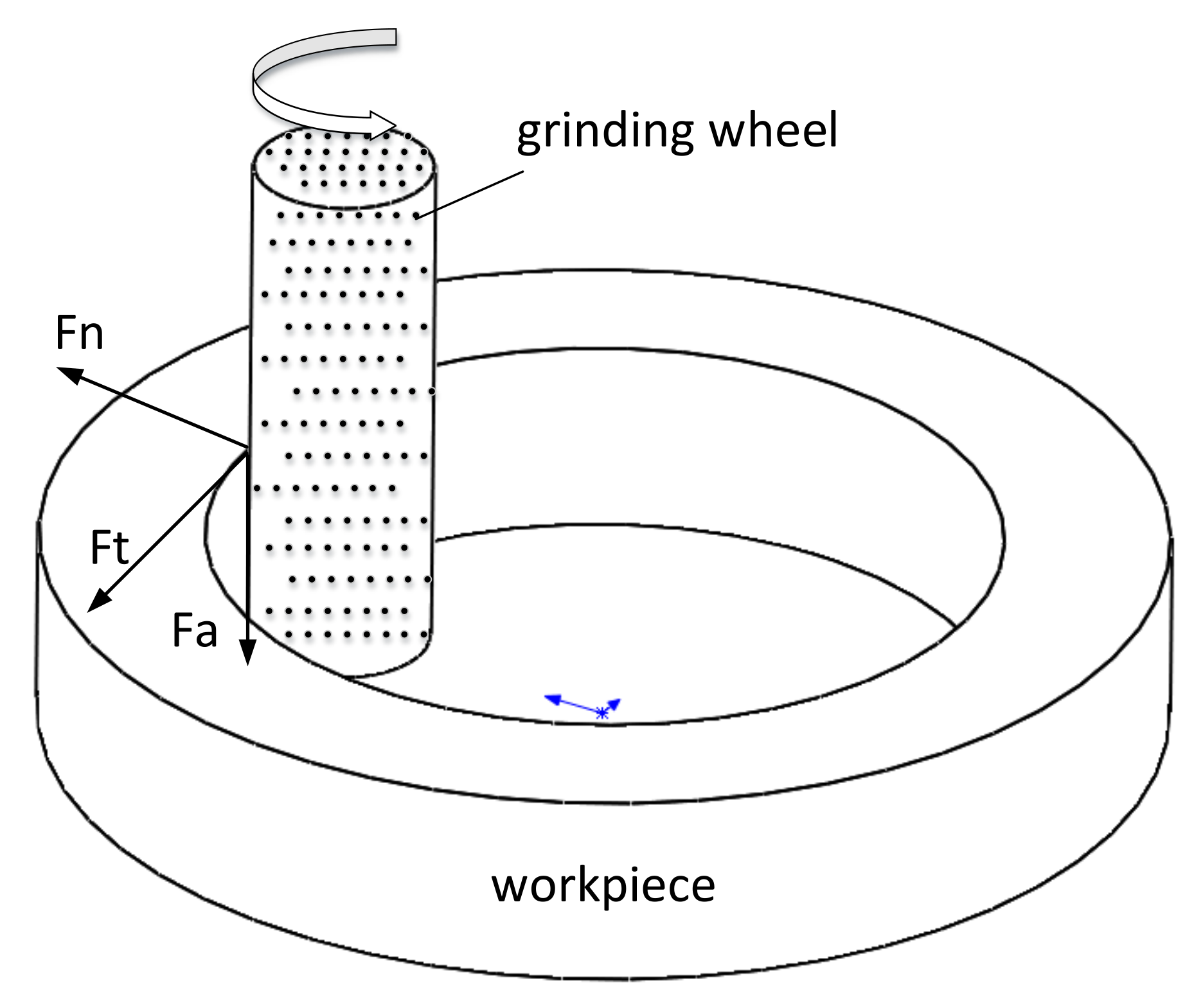
2. Analysis of the Grinding Force in the Inner Circle of the Centrifugal Pump Shell

The grinding force generated in the grinding and polishing process can usually be decomposed into three forces perpendicular to each other, namely the tangential grinding force $F_t$ along the tangential direction of the grinding wheel, the normal grinding force $F_n$ along the radial direction of the grinding wheel, and the axial friction $F_a$ along the axial direction of the grinding wheel. The grinding force generated during internal grinding and polishing is shown in Figure 1.

In the process of grinding and polishing in the inner circle of the centrifugal pump shell, the axial grinding force $F_a$ is small and can be ignored. Since the abrasive grains on the grinding wheel have a large negative rake angle, the normal grinding force $F_n$ is greater than the tangential grinding force $F_t$. Generally, $\frac{F_n}{F_t}$ is in the range of 1.5 ~ 3 (referred to as the grinding ratio). Therefore, controlling the normal grinding force in the inner circle is equivalent to controlling the grinding force in the grinding and polishing process of the centrifugal pump shell.

The empirical formula of the tangential grinding force is [33]:

$$F_t=169f_r^{0.62}{f}_{av}^{0.44}{v}_w^{0.69}$$

(1)

where $f_r$ is the grinding (radial) depth, mm; $f_{av}$ is the axial feed speed, m/min; and $v_w$ is the linear speed of workpiece rotation, m/min.

According to the grinding conditions, the tangential grinding force was calculated from Equation (1) and then the normal grinding force was calculated according to the grinding ratio, which can be used as the expected input force for contact force control in the grinding process.

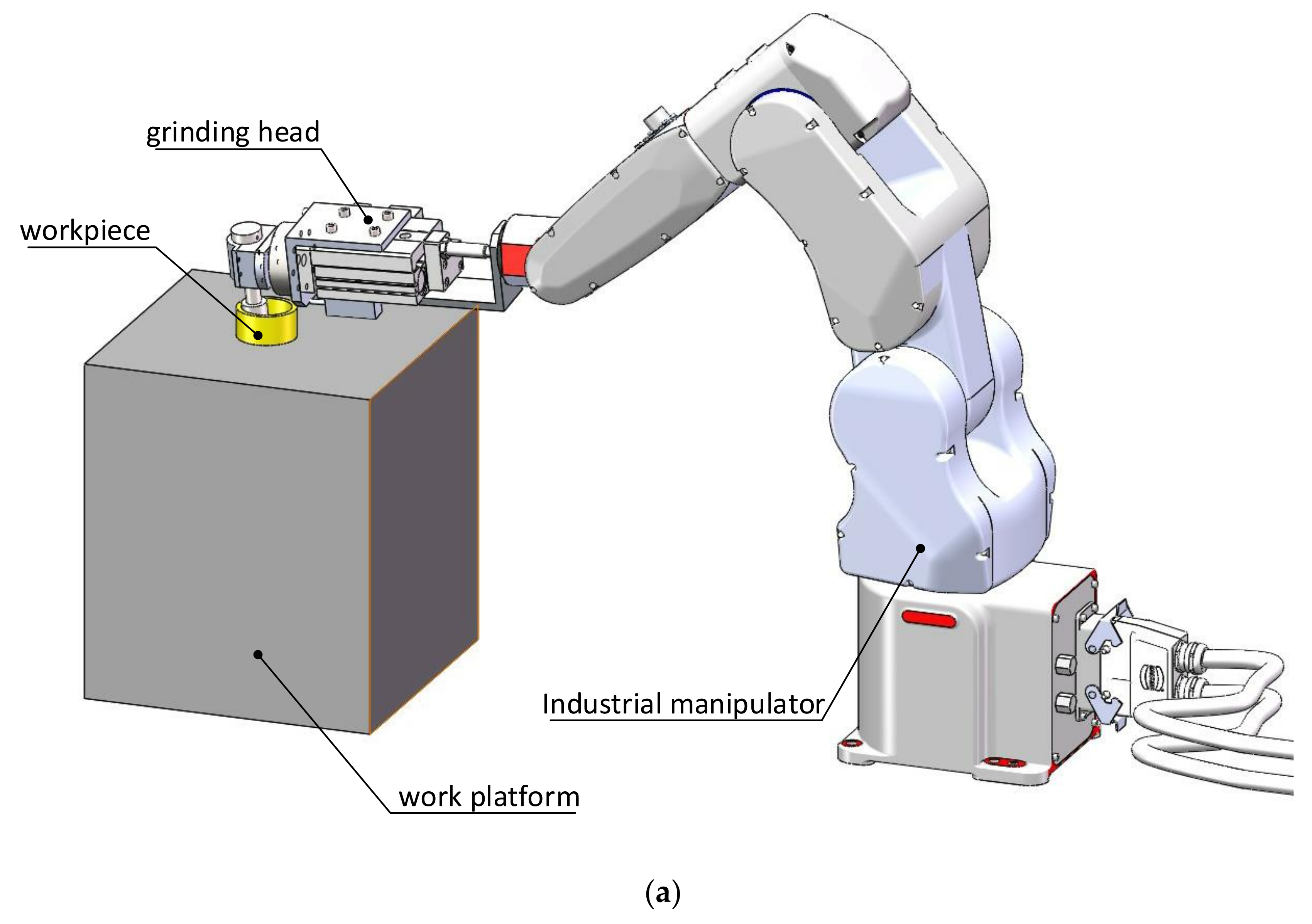
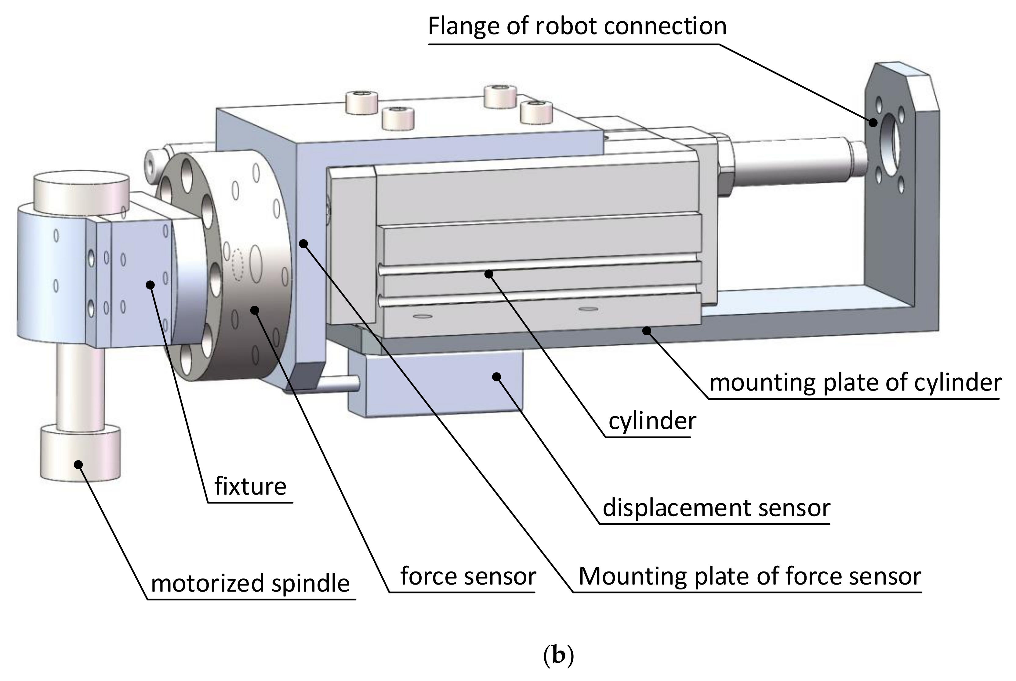
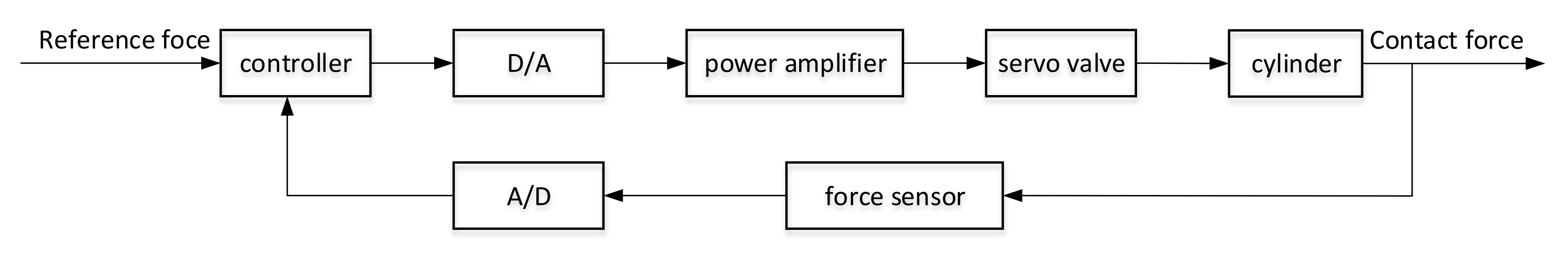
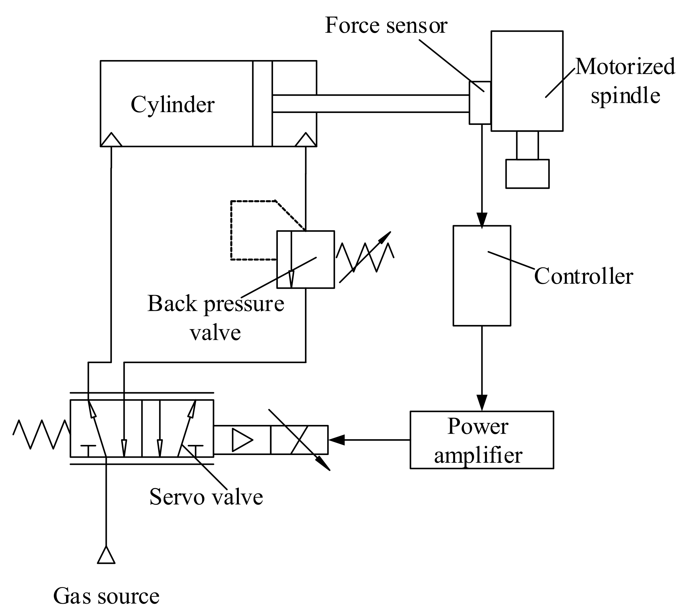
3. Design of the Grinding Force Control System

Figure 2 shows the three-dimensional model of the grinding system. Figure 2a is the layout of the grinding system, and Figure 2b is the composition structure of the grinding device. the grinding device is installed on the robot wrist, which is mainly composed of a motorized spindle, fixture, force sensor, mounting plate for the force sensor, displacement sensor, mounting plate for the cylinder, and flange for robot connection. In order to realize the constant output of the grinding force, the grinding force is detected by the force sensor and transmitted to the controller in the grinding process, which controls the pneumatic proportional valve to adjust the output force of the cylinder.

In the pneumatic control system, the controller converts the expected grinding force into the control quantity of the solenoid valve and controls the solenoid valve to output the normal grinding force through D/A conversion and power amplification. In the feedback, the grinding force signal is detected by the force sensor, converted by A/D, and compared with the expected grinding force, and the control algorithm is designed to adjust in order to keep the output grinding force constant. A block diagram of the pneumatic control system of the robot grinding and polishing device is shown in Figure 3.

Figure 4 is a schematic diagram of the pneumatic control system based on the VER servo valve. By adjusting the control voltage of the servo valve, the pressure difference between the rodless cavity and the rod cavity of the cylinder is changed to drive the piston of the cylinder, causing the grinding head to come into contact with the centrifugal pump shell. The force sensor feeds back the force signal to the controller. The controller adjusts the pressure difference between the two cavities of the throttle cylinder by adjusting the electrical signal of the electric servo valve, which can realize the constant grinding force. The servo valve control system can efficiently and accurately control the polishing force and it has the characteristics of a fast response speed and high precision of control.

4. Modeling of the Pneumatic Servo System

In order to analyze the characteristics of the pneumatic servo system of the centrifugal pump shell in the robot grinding and polishing device, a mathematical model of the pneumatic servo system needs to be established. The following describes the establishment of the mathematical model of the servo system.

When modeling the pneumatic servo system, the following assumptions are made [34]:

(1)

The working medium is assumed to be an ideal gas and all parameters are applicable to the state equation of ideal gas;

(2)

During the working process, there is no heat exchange between the gas inside and outside the cylinder cavity;

(3)

The air source pressure is constant, and the atmospheric pressure and air source temperature are also constant;

(4)

The thermodynamic change process is a quasi-static process in the cylinder cavity;

(5)

The leakage of the cylinder is ignored;

(6)

In the dynamic process of the system, the change in gas inertia force caused by the change in gas velocity is ignored.

4.1. Cylinder Flow Continuity Equation

According to the law of mass conservation, the mass flow of the gas in the cylinder cavity should be the mass change rate of the gas in the cylinder cavity, namely

$$\left\{\begin{array}{l}{q}_{m_1}=\frac{d{m}_1}{dt}\\ q_{m_2}=\frac{d{m}_2}{dt}\end{array}\right.$$

(2)

where $q_{m_1}$ is the gas mass flow in the rodless cavity of the cylinder, $q_{m_2}$ is the gas mass flow in the rod cavity of the cylinder, $m_1$ is the gas mass in the rodless cavity of the cylinder, and $m_2$ is the gas mass in the rod cavity of the cylinder.

The state equation of the ideal gas in equilibrium is

$$pV=mRT$$

(3)

where $p$ is the absolute pressure of gas, Pa; $V$ is the gas volume, ${\mathrm{m}}^3$; $m$ is the gas mass, kg; $R$ is the gas constant, dry air: $R=287.1\mathrm{N}\cdot \mathrm{m}/(\mathrm{kg}\cdot K)$; and $T$ is the thermodynamic temperature of gas, K.

From Equation (3)

$$m=\frac{pV}{RT}$$

(4)

Equation (4) can be substituted into Equation (2) to obtain

$$\left\{\begin{array}{l}{q}_{m_1}=\frac{d{m}_1}{dt}=\frac{1}{RT}\left(p_1\frac{d{V}_1}{dt}+V_1\frac{d{p}_1}{dt}-\frac{p_1{V}_1}{T_1}\frac{d{T}_1}{dt}\right)\\ q_{m_2}=\frac{d{m}_2}{dt}=\frac{1}{RT}\left(p_2\frac{d{V}_2}{dt}+V_2\frac{d{p}_2}{dt}-\frac{p_2{V}_2}{T_2}\frac{d{T}_2}{dt}\right)\end{array}\right.$$

(5)

where $q_{m_1},q_{m_2}$ is the mass flow of the two chambers of the cylinder, $\mathrm{kg}/\mathrm{s}$; $\frac{d{T}_1}{dt},\frac{d{T}_2}{dt}$ is the temperature change rate of the two chambers of the cylinder, $\mathrm{K}/\mathrm{s}$; $\frac{d{p}_1}{dt},\frac{d{p}_2}{dt}$ is the pressure change rate of the two chambers of the cylinder, $\mathrm{Pa}/\mathrm{s}$; $\frac{d{V}_1}{dt},\frac{d{V}_2}{dt}$ is the volume change rate of the two chambers of the cylinder, ${\mathrm{m}}^3/\mathrm{s}$; $V_1,V_2$ is the volume of the two chambers of the cylinder, ${\mathrm{m}}^3$; $p_1,p_2$ is the pressure of the two chambers of the cylinder, $\mathrm{Pa}$; and $T$ is the thermodynamic temperature of the cylinder, $\mathrm{K}$.

According to the above assumptions, during the movement of the cylinder, the change process of the gas in the cylinder is an isentropic process, which is an adiabatic process, and the adiabatic equation is

$$p^{k-1}{T}^{-k}=C$$

(6)

where $k$ is the gas isentropic index, for air: $k=1.4$.

By deriving Equation (6) from time, we get

$$\frac{dT}{dt}=\frac{(k-1)T}{kp}\frac{dp}{dt}$$

(7)

Substituting Equation (7) into Equation (5), we can find the mass flow of the two cylinder cavities, so that

$$\left\{\begin{array}{l}{q}_{m_1}=\frac{1}{R{T}_1}\left(p_1\frac{d{V}_1}{dt}+\frac{V_1}{k}\frac{d{p}_1}{dt}\right)\\ q_{m_2}=\frac{1}{R{T}_2}\left(p_2\frac{d{V}_2}{dt}+\frac{V_2}{k}\frac{d{p}_2}{dt}\right)\end{array}\right.$$

(8)

According to the assumption that the gas temperature in the cylinder cavity is the same as the ambient temperature and the air source temperature, which are also constant, it can be expressed by $T_0$. Then, Equation (8) becomes

$$\left\{\begin{array}{l}{q}_{m_1}=\frac{1}{R{T}_0}\left(p_1\frac{d{V}_1}{dt}+\frac{V_1}{k}\frac{d{p}_1}{dt}\right)\\ q_{m_2}=\frac{1}{R{T}_0}\left(p_2\frac{d{V}_2}{dt}+\frac{V_2}{k}\frac{d{p}_2}{dt}\right)\end{array}\right.$$

(9)

The pressure dynamic equation of the two cylinder cavities is

$$\left\{\begin{array}{l}\frac{d{p}_1}{dt}=\frac{kR{T}_0}{V_1}{q}_{m_1}-\frac{k{p}_1}{V_1}\frac{d{V}_1}{dt}\\ \frac{d{p}_2}{dt}=\frac{kR{T}_0}{V_2}{q}_{m_1}-\frac{k{p}_2}{V_2}\frac{d{V}_2}{dt}\end{array}\right.$$

(10)

In the pneumatic servo system of the robot grinding and polishing device, the grinding force is controlled by the cylinder, and the spatial position motion is completed by the robot. When the robot positioning error is very small, the grinding wheel is always in contact with the workpiece, so the displacement of the piston rod is very small. In the process of practical application, the influence of the displacement of the cylinder piston rod on the flow is ignored. The mass flow equation of the two cylinder cavities can be simplified as follows from Equation (9):

$$\left\{\begin{array}{l}{q}_{m_1}=\frac{1}{R{T}_0}\frac{V_1}{k}\frac{d{p}_1}{dt}\\ q_{m_2}=\frac{1}{R{T}_0}\frac{V_2}{k}\frac{d{p}_2}{dt}\end{array}\right.$$

(11)

4.2. Mass Flow Equation of the Pneumatic Servo Valve

The flow process of the gas passing through the valve port of the servo valve is relatively complex. Generally, the flow process of the gas passing through the valve port of a proportional servo valve is considered to be the one-dimensional isentropic flow of an ideal gas. According to the Sanville flow formula [35], the mass flow formula of a proportional valve port is

$$q_m=\mu A_t{P}_u\sqrt{\frac{2}{RT}}\Phi \left(\frac{P_d}{P_u}\right)$$

(12)

$$\Phi \left(\frac{P_d}{P_u}\right)=\left\{\begin{array}{ll}\sqrt{\frac{k}{k-1}}\left[{\left(\frac{P_d}{P_u}\right)}^{\frac{2}{k}}-{\left(\frac{P_d}{P_u}\right)}^{\frac{k+1}{k}}\right]& 0.528<\frac{P_d}{P_u}\le 1\\ \sqrt{\frac{k}{k+1}{\left(\frac{2}{k+1}\right)}^{\frac{2}{k-1}}}& 0\le \frac{P_d}{P_u}\le 0.528\end{array}\right.$$

where $q_m$ is the mass flow of the servo valve port, $\mathrm{kg}/\mathrm{s}$; $A_t$ is the opening area of the valve port, m²; $\mu$ is the flow coefficient; R is the gas constant; $P_u$ is the absolute pressure upstream of the valve port, Pa; $P_d$ is the absolute pressure downstream of the valve port, Pa; and k is the gas isentropic index.

The opening area of the servo valve is

$$A_t=\omega x_v$$

(13)

where $x_v$ is the valve core displacement, m, and $\omega$ is the area gradient of the valve port ($\omega =\pi D$), m.

Equation (13) can be substituted into Equation (12) to get:

$$q_m=\mu \pi D{x}_v{P}_u\sqrt{\frac{2}{RT}}\Phi \left(\frac{P_d}{P_u}\right)$$

(14)

Then, the inlet flow and outlet flow of the valve are, respectively:

$$\left\{\begin{array}{l}{q}_{m_1}=\mu \pi D{x}_v{P}_p\sqrt{\frac{2}{RT}}\Phi \left(\frac{P_1}{P_p}\right)\\ q_{m_2}=\mu \pi D{x}_v{P}_2\sqrt{\frac{2}{RT}}\Phi \left(\frac{P_k}{P_2}\right)\end{array}\right.$$

(15)

where $P_p$ is the air source pressure, Pa; $P_1$ is the pressure without a rod chamber, Pa; $P_2$ is the pressure with a rod chamber, Pa; and $P_k$ is the atmospheric pressure, Pa.

Since the displacement of the proportional valve spool is linear with the input voltage u [11], $x_v=K_{u}u$, $K_u$ is the gain coefficient of the proportional valve. Then, we get

$$\left\{\begin{array}{l}{q}_{m_1}=\mu \pi D{K}_{u}u{P}_p\sqrt{\frac{2}{RT}}\Phi \left(\frac{P_1}{P_p}\right)\\ q_{m_2}=\mu \pi D{K}_{u}u{P}_2\sqrt{\frac{2}{RT}}\Phi \left(\frac{P_k}{P_2}\right)\end{array}\right.$$

(16)

It can be seen from the above formula that the actual flow at the valve port is related to the pressure at the air outlet and the control voltage of the electric servo valve, so the flow formula can be simplified as

$$q_m=f(u,P)$$

(17)

where u is the control voltage of the servo valve.

Equation (16) can be linearized near the zero position to obtain

$$\left\{\begin{array}{l}{q}_{m_1}=K_1\Delta u-K_2\Delta p_1\\ q_{m_2}=K_3\Delta u+K_4\Delta p_2\end{array}\right.$$

(18)

$$K_1={\left.\frac{\partial q_{m_1}}{\partial u}\right|}_{\begin{array}{l}u=0\\ p_1=P_{10}\end{array}},K_2={\left.\frac{\partial q_{m_1}}{\partial p_1}\right|}_{\begin{array}{l}u=0\\ p_1=P_{10}\end{array}},K_3={\left.\frac{\partial q_{m_2}}{\partial u}\right|}_{\begin{array}{l}u=0\\ p_2=P_{20}\end{array}},K_4={\left.\frac{\partial q_{m_2}}{\partial p_2}\right|}_{\begin{array}{l}u=0\\ p_2=P_{20}\end{array}}$$

where

$$\begin{gathered} \begin{array}{l}{K}_1={\left.\frac{\partial q_{m_1}}{\partial u}\right|}_{\begin{array}{l}u=0\\ p_1=P_{10}\end{array}}={\left.\mu \pi D{K}_u{P}_p\sqrt{\frac{2}{RT}}\Phi \left(\frac{P_1}{P_p}\right)\right|}_{\begin{array}{l}u=0\\ p_1=P_{10}\end{array}}=\mu \pi D{K}_u{P}_p\sqrt{\frac{2}{RT}}\sqrt{\frac{k}{k-1}}\left[{\left(\frac{P_1}{P_p}\right)}^{\frac{2}{k}}-{\left(\frac{P_1}{P_p}\right)}^{\frac{k+1}{k}}\right],\\ K_2={\left.\frac{\partial q_{m_1}}{\partial p_1}\right|}_{\begin{array}{l}u=0\\ p_1=P_{10}\end{array}}=0,\end{array} \\ \begin{array}{l}{K}_3={\left.\frac{\partial q_{m_2}}{\partial u}\right|}_{\begin{array}{l}u=0\\ p_2=P_{20}\end{array}}={\left.\mu \pi D{K}_u{P}_2\sqrt{\frac{2}{RT}}\Phi \left(\frac{P_k}{P_2}\right)\right|}_{\begin{array}{l}u=0\\ p_2=P_{20}\end{array}}=\mu \pi D{K}_u{P}_2\sqrt{\frac{2}{RT}}\sqrt{\frac{k}{k-1}}\left[{\left(\frac{P_a}{P_2}\right)}^{\frac{2}{k}}-{\left(\frac{P_a}{P_2}\right)}^{\frac{k+1}{k}}\right],\\ K_4={\left.\frac{\partial q_{m_2}}{\partial p_2}\right|}_{\begin{array}{l}u=0\\ p_2=P_{20}\end{array}}=0.\end{array} \end{gathered}$$

where $P_{10},P_{20}$ is the pressure of the rodless chamber and the rod chamber when the piston is balanced; $\Delta u$ is the variation of voltage; $\Delta p_1,\Delta p_2$ is the variation of pressure of the two chambers of the cylinder.

4.3. Force Balance Equation of the Cylinder

The force of the cylinder of the pneumatic system in the robot grinding and polishing device was analyzed according to Newton’s second law and the force balance equation of the cylinder was obtained as

$$P_1{A}_1-P_2{A}_2-F_f-F_L=M\frac{d^{2}y}{d{t}^2}+f\frac{dy}{dt}+K_{p}y$$

(19)

where $A_1,A_2$ is the area of the piston in the two chambers of the cylinder, ${\mathrm{m}}^2$; $P_1,P_2$ is the pressure of the two chambers of the cylinder, Pa; $F_L$ is the actual grinding and polishing force, N; $F_f$ is the friction force on the cylinder, N; M is the total mass of all parts of the cylinder, kg; f is the viscous damping coefficient; K_P is the cylinder spring stiffness; and y is the output displacement of the cylinder.

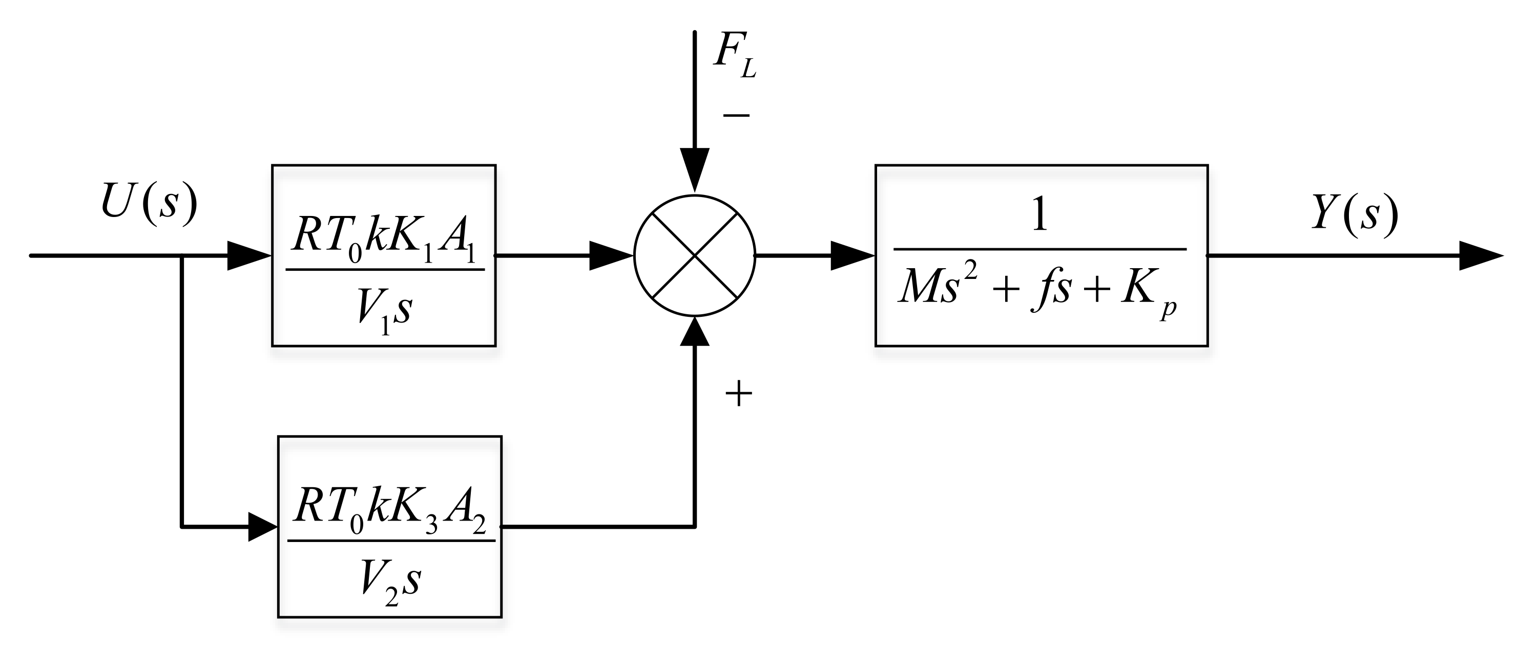
4.4. Establishment of a Mathematical Model of the Pneumatic System of the Robot Grinding and Polishing Device

By applying the Laplace transformation to Equations (11) and (18), we get

$$\left\{\begin{array}{l}{Q}_{m_1}(s)=\frac{1}{R{T}_0}\frac{V_1}{k}s{P}_1(s)\\ Q_{m_2}(s)=\frac{1}{R{T}_0}\frac{V_2}{k}s{P}_2(s)\end{array}\right.$$

(20)

$$\left\{\begin{array}{l}{Q}_{m_1}(s)=K_{1}U(s)\\ Q_{m_2}(s)=K_{3}U(s)\end{array}\right.$$

(21)

Simultaneously, for Equations (20) and (21), we get

$$\left\{\begin{array}{l}\frac{P_1(s)}{U(s)}=\frac{R{T}_{0}k{K}_1}{V_{1}s}\\ \frac{P_2(s)}{U(s)}=\frac{R{T}_{0}k{K}_3}{V_{2}s}\end{array}\right.$$

(22)

From the Laplace transformation of the cylinder force balance equation, Equation (19), we get

$$M{s}^{2}Y(s)+fsY(s)+K_{p}Y(s)=P_1(s)A_1-P_2(s)A_2-F_f(s)-F_L(s)$$

(23)

If we ignore the friction and let $F_L(s)=0$, the transfer function of the cylinder piston displacement and the proportional valve input voltage obtained from Equations (20)–(23) is

$$\frac{Y(s)}{U(s)}=\frac{b_0}{a_3{s}^3+a_2{s}^2+a_{1}s}$$

(24)

where

$$\left\{\begin{array}{l}{b}_0=R{T}_{0}k(K_1{A}_1{V}_2-K_3{A}_2{V}_1)\\ a_3=M{V}_1{V}_2\\ a_2=f{V}_1{V}_2\\ a_1=K_p{V}_1{V}_2\\ K_p=\frac{4k{P}_1{A}_1}{l}\end{array}\right.$$

Let $U(s)=0$; the transfer function between the cylinder piston displacement and the input load force is

$$\frac{Y(s)}{F_n(s)}=\frac{-1}{M{s}^2+fs+K_p}$$

(25)

The transfer function between the cylinder piston displacement and the grinding force is

$$\frac{Y(s)}{F_n(s)}=\frac{1}{M{s}^2+fs+K_p}$$

(26)

If the input load force value of the pneumatic system is equal to the output force value of the pneumatic system, and the direction of the force is opposite, the transfer function between the load force of the grinding and polishing device and the input voltage of the proportional valve is

$$\frac{F(s)}{U(s)}=\frac{\left(M{s}^2+fs+K_p\right)b_0}{a_3{s}^3+a_2{s}^2+a_{1}s}=\frac{\left(M{s}^2+fs+K_p\right)b_0}{s(a_3{s}^2+a_{2}s+a_1)}$$

(27)

According to Equation (27), the aerodynamic control system of the robot grinding and polishing device is composed of the proportional link, second-order differential link, integral link, and second-order oscillation link.

Based on Equations (22) and (23), a block diagram representing the transfer function of the pneumatic system of the grinding device is shown in Figure 5.

In practical engineering applications, the force sensor is used to detect the load force, and the displacement sensor is used to detect the movement displacement of the cylinder piston, so as to realize closed-loop control. The block diagram is shown in Figure 6.

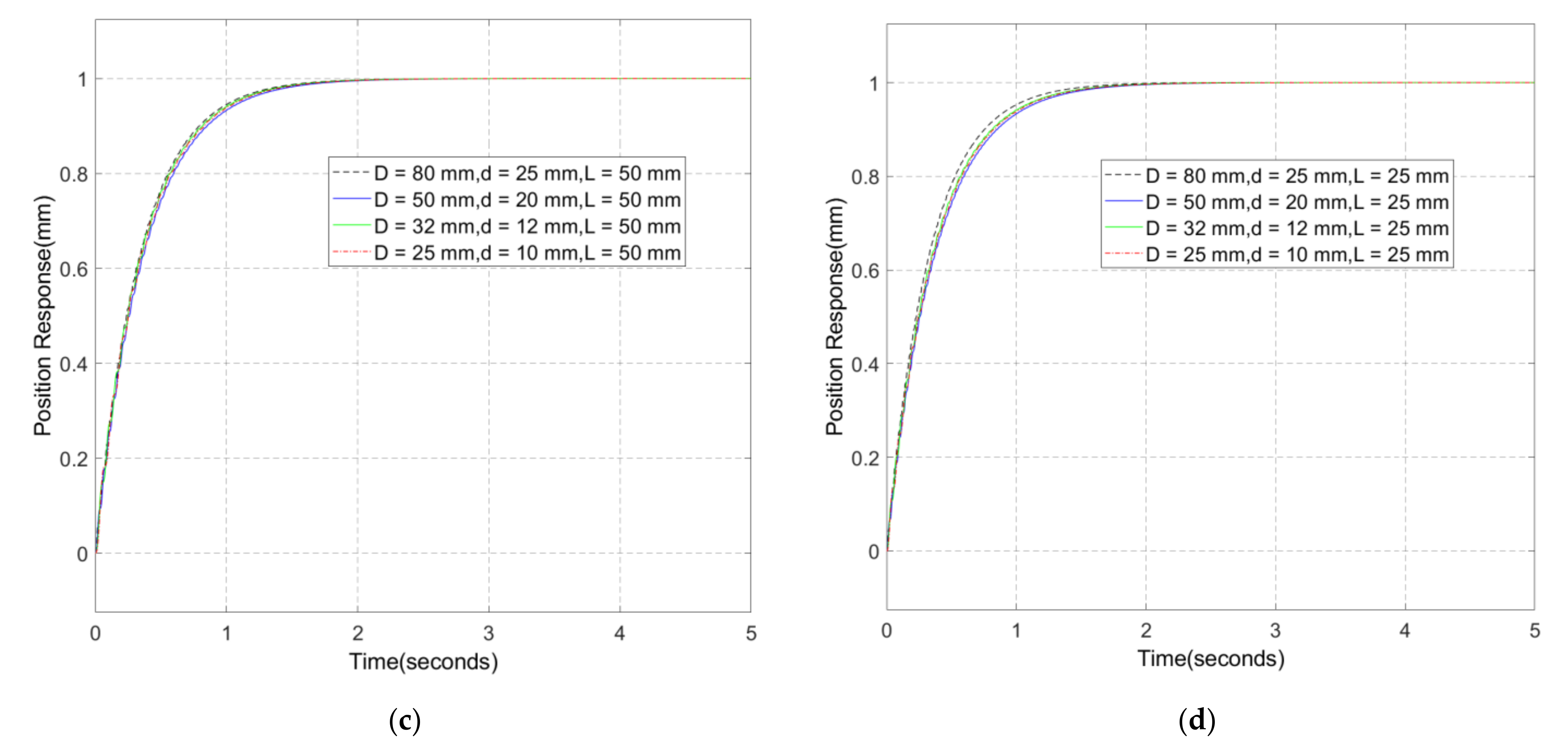
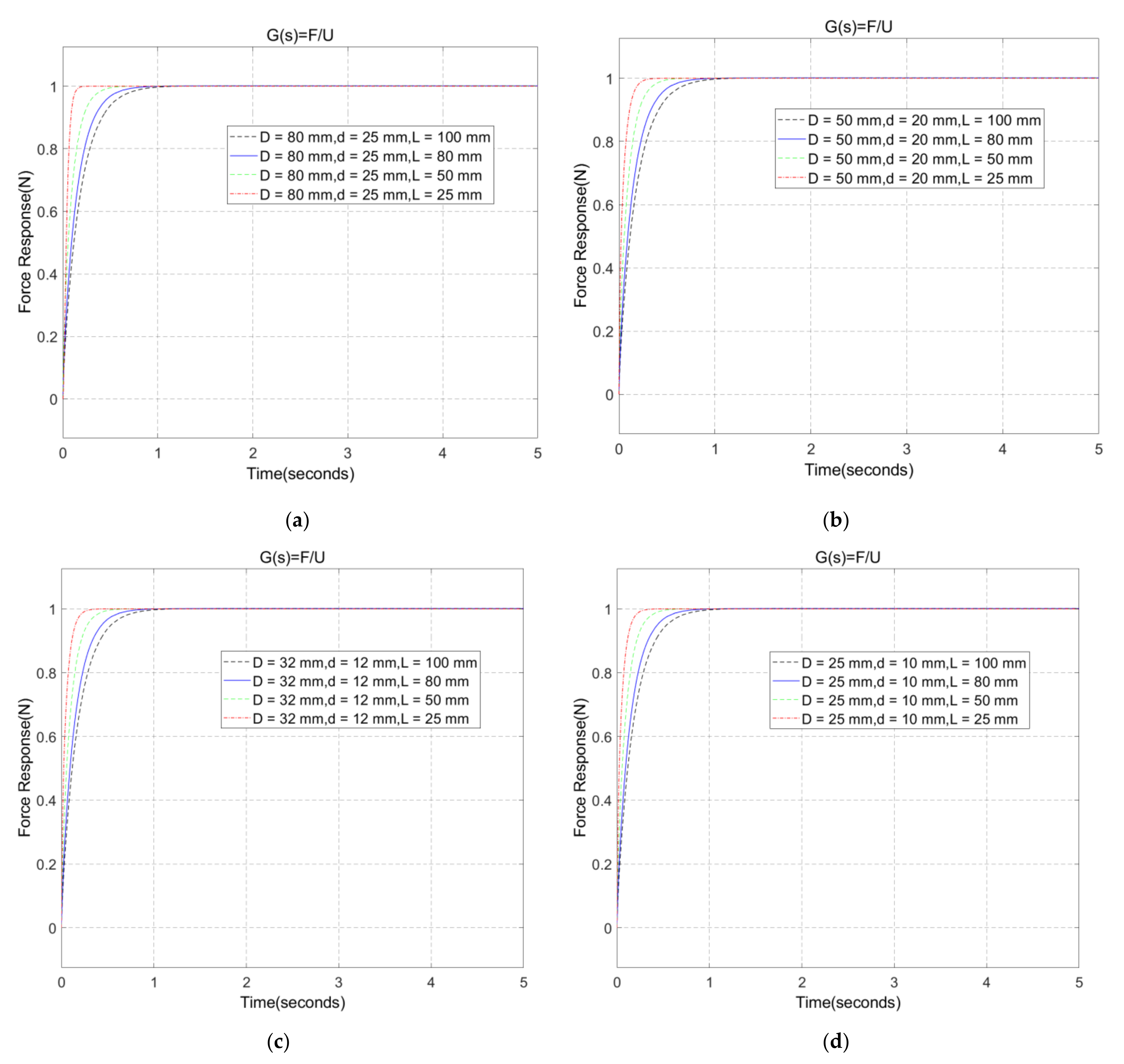
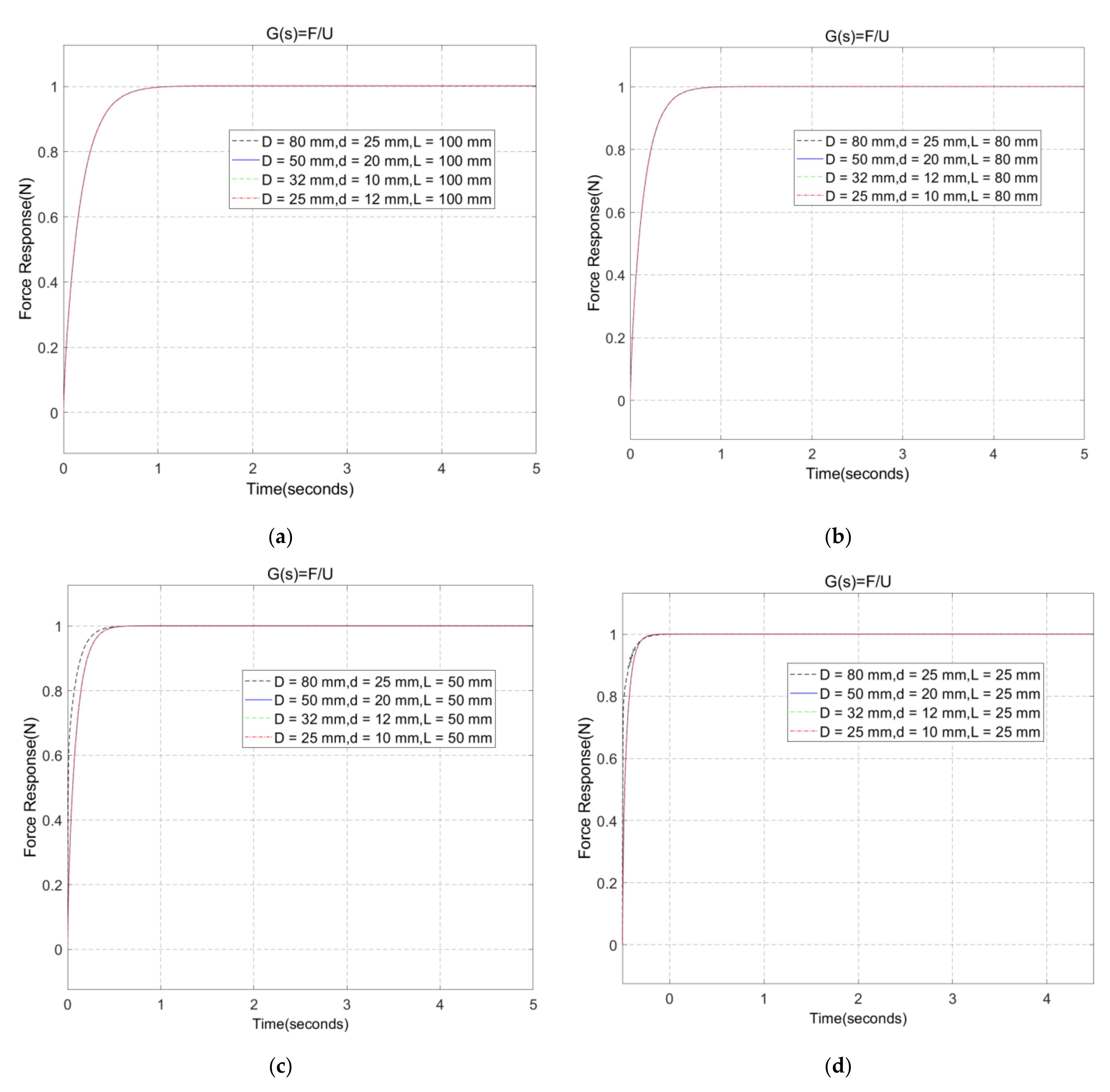
4.5. Design and Analysis of the Structural Parameters of the Pneumatic System

In the pneumatic control system of the centrifugal pump shell, the load mass is 5 kg, the air source pressure is $P_s=0.7\mathrm{MPa}$, the atmospheric pressure is $P_a=0.1\mathrm{MPa}$ and the pressure difference between the front and rear of the valve port is 0.02MPa. The relevant parameters of the pneumatic servo control system at the balance position are shown in

Table 1. Relevant parameters of the pneumatic servo system.

Parameters	Numerical Value
Load mass M (Kg)	5
Gas constant R (J/(Kg K)	287.1
Temperature T0 (K)	298
Heat transfer constant k	1.4
Viscous damping coefficient f	50
Discharge coefficient u	0.628
Gain coefficient of valve Ku	0.2
Coefficient K1	0.1582
Coefficient K2	0
Coefficient K3	0.134
Coefficient K4	0

. The structural parameters of the different cylinders are shown in

Table 2. Structural parameters of the different cylinders.

		Stroke	100 mm	80 mm	50 mm	25 mm
	Rod Diameter
Cylinder Diameter
80 mm			25 mm	25 mm	25 mm	25 mm
50 mm			20 mm	20 mm	20 mm	20 mm
32 mm			12 mm	12 mm	12 mm	12 mm
25 mm			10 mm	10 mm	10 mm	10 mm

.

According to the above transfer function, it can be seen that the pneumatic control system of the robot grinding and polishing device is a complex third-order system, and the parameters of the system are related to many factors, such as the structure, temperature, and load of the electric servo value. Substituting the parameters in Table 1 and Table 2 into Equations (24), (26), and (27), we can obtain the transfer functions of the pneumatic control system of the robot grinding and polishing device in cylinders with different structural parameters.

5. Stability Analysis of the Pneumatic Control System of the Robot Grinding and Polishing Device

Stability is an important characteristic of the control system of the robot grinding and polishing device. For the control system of the robot grinding and polishing device to work normally, the system must initially be a stable system, that is, after the control system of the robot grinding and polishing device is disturbed by the external force, the original equilibrium state of the control system is broken. However, the pneumatic control system of the robot grinding and polishing device should have the ability to automatically return to the original equilibrium state or tend to another new equilibrium state and continue to work after the external force disturbance disappears. The stability of the control system of the robot grinding and polishing device was analyzed using the Hurwitz method and the steady-state error of the control system of the robot grinding and polishing device was calculated, as demonstrated in the following sections.

5.1. Stability Analysis of the Control System of the Robot Grinding and Polishing Device

For the pneumatic control system of the centrifugal pump shell robot grinding and polishing device, firstly, the Hurwitz method was used to analyze whether the system was stable, so as to clarify the stability performance of the control system.

The characteristic equation of the system is

$$a_n{s}^n+a_{n-1}{s}^{n-1}+a_{n-2}{s}^{n-2}+\cdots +a_0=0(a_n>0,n=0,1,2,\cdots n)$$

(28)

According to the Hurwitz criterion, we arrange the characteristic equation coefficients of Equation (28) into the Hurwitz matrix, so that

$$H=\left[\begin{array}{cccccc}{a}_{n-1}& a_{n-3}& a_{n-5}& \cdots & 0& 0\\ a_n& a_{n-2}& a_{n-4}& \cdots & 0& 0\\ 0& a_{n-1}& a_{n-3}& \cdots & 0& 0\\ 0& a_n& a_{n-2}& \cdots & 0& 0\\ ⋮& ⋮& ⋮& ⋮& ⋮& ⋮\\ 0& 0& 0& \cdots & 0& a_0\end{array}\right]$$

(29)

If the principal sub-formulas of each order of the Hurwitz matrix are greater than zero, that is, $\det (H_n)>0(n=1,2,3,\cdots n)$, then the system is stable.

According to the structural parameters of different cylinders, the characteristic equation of the system can be obtained based on the system transfer function, so that

$$\det (H_n)>0(n=1,2,3)$$

(30)

According to the above analysis, the principal sub-formulas of each order of the Hurwitz matrix, which are composed of the coefficients of each order of the characteristic equation of the system, are greater than zero, so the system is stable.

For the cylinders with different diameters and strokes, the step function was used as the input to obtain the position output response of the system. Figure 7 shows the output response curve of the cylinder position with different strokes and the same cylinder diameter. As can be seen in Figure 7, when the cylinder diameter D = 80 mm and the piston rod diameter d = 25 mm, the cylinder position response is not affected by the stroke. The transition is stable and the transition time is approximately 20 s. When the cylinder diameter D = 50 mm and the piston rod diameter d = 20 mm, the oscillation intensifies in the transition stage. After reaching stability, the position response is relatively stable and the transition time is approximately 8 s. When the cylinder diameter D = 32 mm and the piston rod diameter d = 12 mm, the oscillation in the transition stage is intense, there is still a little oscillation after stability is reached, and the time to reach stability becomes longer, for approximately 3 s. When the double cylinder is adopted, with a cylinder diameter D = 25 mm and a piston rod diameter d = 10 mm, there is oscillation in the transition stage. Stability is reached with a transition time of approximately 1.5 s. Figure 8 shows the output response curve of the cylinder position with different cylinder diameters in the same stroke. As can be seen in the Figure 8, the larger the diameter of the single shaft cylinder, the more stable the position output, and the longer the transition time.

The force output response curves are shown in Figure 9 and Figure 10. Figure 9 shows the output force response curves of different strokes and Figure 10 shows the output force response curves of different cylinder diameters. According to Figure 9a,b, when the cylinder diameter D = 80 mm and the piston rod diameter d = 25 mm, the greater the stroke, the greater the oscillation amplitude, but the time to reach stability is basically the same, being approximately 0.3 s. It can be seen in Figure 9c,d that the time to reach stability is approximately 0.4 s when the cylinder diameter D = 50 mm and the piston rod diameter d = 20 mm, and the oscillation amplitude is the smallest when the stroke L = 25 mm. It can be seen in Figure 9e,f that the oscillation amplitude is the largest when the cylinder diameter D = 32 mm, the piston rod diameter d = 12 mm, and the stroke L = 80 mm. According to Figure 9g,h, when the cylinder diameter D = 25 mm and the piston rod diameter d = 10 mm, the greater the stroke, the greater the oscillation amplitude. According to Figure 10a–c, when the cylinder diameter D = 50 mm and the piston rod diameter d = 20 mm, the oscillation amplitude is the largest. Figure 10d shows that the oscillation is obvious when the cylinder diameter D = 80 mm and the piston rod diameter d = 25 mm, and others have almost no oscillation. As can be seen in Figure 9 and Figure 10, the force output response has impact and oscillation in the initial stage, which needs to be corrected in order to obtain constant force control.

5.2. Steady-State Error Analysis of the Pneumatic Control System of the Robot Grinding Device

The steady-state error of the pneumatic control system of the centrifugal pump housing in the robot grinding device is an important technical index, which reflects the accuracy of the system. The steady-state error of the pneumatic control system is related not only to the form of external action but also to the structural parameters of the control system itself. Since the pneumatic control system of the centrifugal pump housing robot grinding device studied in this work is stable, its accuracy needs to be further studied. The stability error of the system is analyzed below.

The feedback control model of the system is shown in Figure 11.

The deviation signal of the system is defined as $\epsilon (s)$, which is shown in Figure 11.

$$\epsilon (s)=U(s)-B(s)=U(s)-H(s)Y(s)$$

(31)

where $U(s)$ is the input signal of the control system; $B(s)$ is the main feedback signal of the control system; $Y(s)$ is the actual output signal of the control system; and $H(s)$ is the transfer function of the main feedback channel.

If the error signal of the system is defined as $E(s)$, then

$$E(s)=Y_r(s)-Y(s)$$

(32)

where $Y_r(s)$ is the desired output signal of the control system.

If $\epsilon (s)=0$, then $Y_r(s)=Y(s)$, and if we substitute this into Equation (29), we get

$$Y_r(s)=\frac{U(s)}{H(s)}$$

(33)

From Equations (31)–(33), we get

$$E(s)=Y_r(s)-Y(s)=\frac{U(s)}{H(s)}-Y(s)=\frac{U(s)-H(s)Y(s)}{H(s)}=\frac{\epsilon (s)}{H(s)}$$

(34)

namely

$$E(s)=\frac{\epsilon (s)}{H(s)}$$

(35)

The steady-state error $e_{ss}$ of the control system is the steady-state component of the system error signal $e(t)$, namely

$$e_{ss}=\underset{t\to \infty }{\lim }e(t)$$

(36)

According to the terminal value theorem of the Laplace transformation, from Equation (36), we get

$$e_{ss}=\underset{t\to \infty }{\lim }e(t)=\underset{s\to 0}{\lim }sE(s)$$

(37)

The transfer function of the error is

$$G_e(s)=\frac{E(s)}{U(s)}$$

(38)

From Equations (31), (35), and (38), we get

$$G_e(s)=\frac{1}{H(s)}\frac{1}{1+G(s)H(s)}$$

(39)

From Equations (37)–(39), we get

$$e_{ss}=\underset{s\to 0}{\lim }s{G}_e(s)U(s)=\underset{s\to 0}{\lim }s\frac{U(s)}{H(s)(1+G(s)H(s))}$$

(40)

It can be seen from Equation (40) that the steady-state error $e_{ss}$ of the control system depends on the structural parameters $G(s)$ and $H(s)$ and the input signals of the system, $U(s)$.

It is assumed that the pneumatic servo control system of the robot polishing device ignores the disturbance, and the input signal of its force control system is a step signal; hence, there is $U(s)=\frac{A}{s}$, where A is the amplitude of the input signal. Then, the steady-state error of the pneumatic control system of the robot grinding device is

$$e_{ss}=\underset{s\to 0}{\lim }s\frac{U(s)}{H(s)(1+G(s)H(s))}=\underset{s\to 0}{\lim }\frac{A}{H(s)(1+G(s)H(s))}$$

(41)

In the unit feedback control system, $H(s)=1$, and from Equations (27) and (41), we get

$$e_{ss}=\underset{s\to 0}{\lim }\frac{A}{1+G(s)}=0$$

(42)

6. Correction and Control of the Pneumatic Servo System

The displacement response of the pneumatic servo system of the robot grinding device (designed shown above) has a too-long rise time when it reaches stability, and there are shocks and oscillations in the initial stage of the force response. These problems seriously affect the performance of the pneumatic servo system and damage the grinding quality of the robot. In order to improve the force control performance of the pneumatic servo system, it is necessary to adopt the corresponding control algorithm to correct the performance of the pneumatic servo system. The following focuses on the PID correction algorithm of displacement and force.

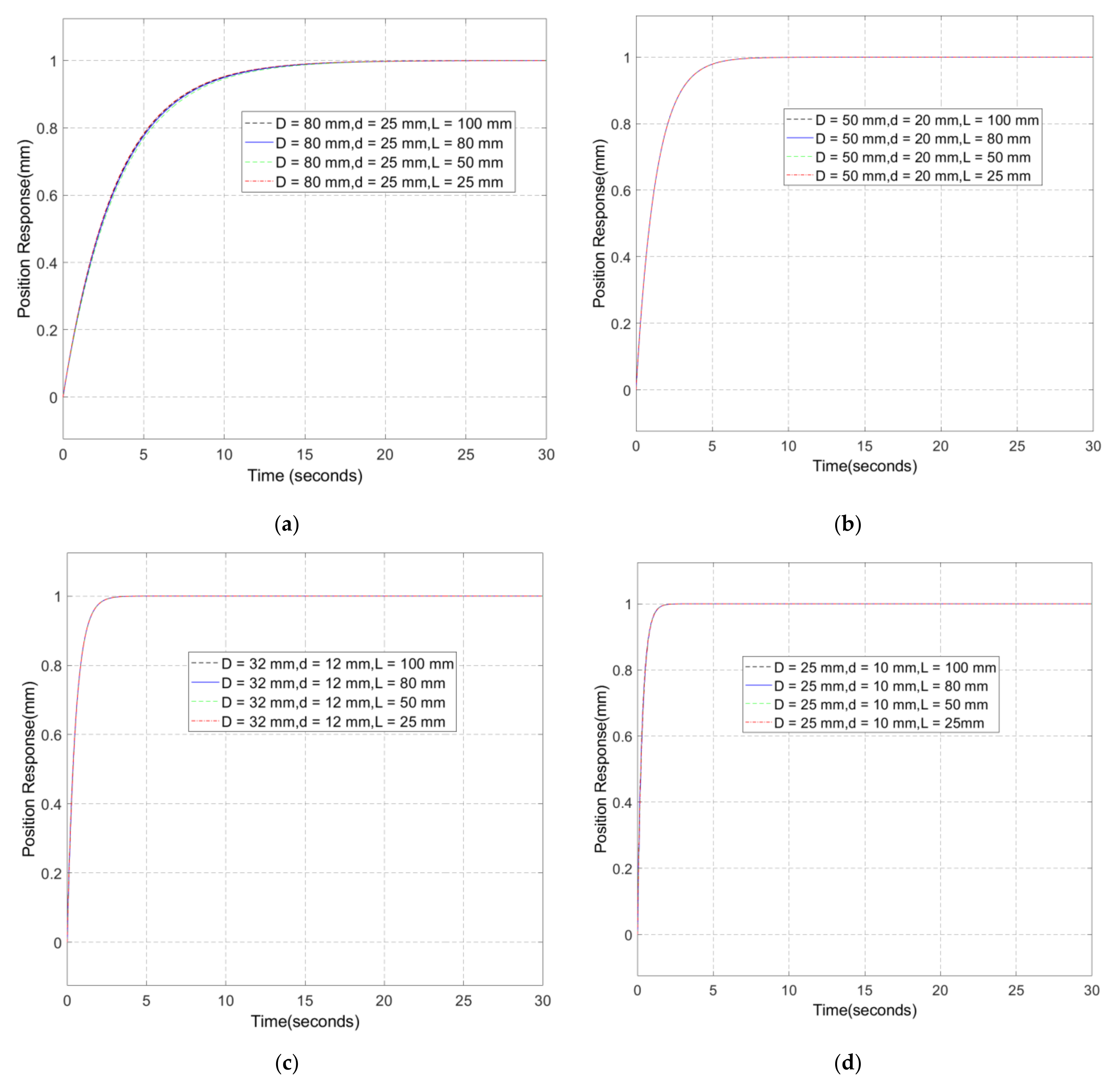
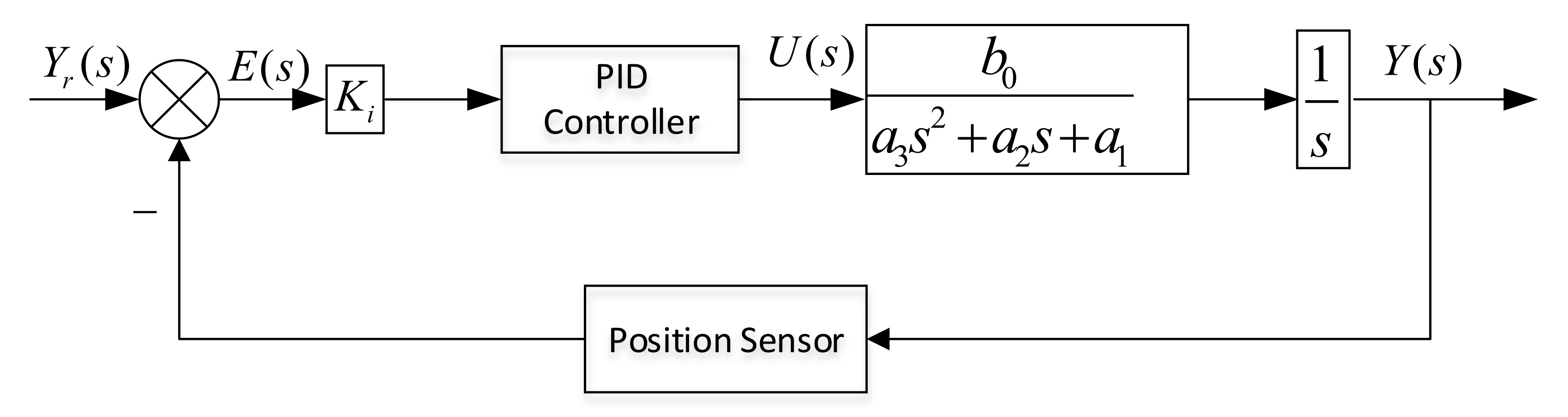
6.1. Displacement Response Correction and Control of the Pneumatic Servo System

On the basis of the pneumatic servo system, the position feedback link and PID controller were added to form the PID control system. The block diagram is shown in Figure 12.

The position response curve based on the displacement feedback PID control is shown in Figure 13 and Figure 14. Figure 13 shows the position response curve for PID control with different strokes. Figure 13a–d show that the time required for the position response to reach stability is approximately 4 s, 2.5 s, 3.5 s, and 2 s when D = 80 mm, 50 mm, 32 mm, and 25 mm, respectively. It can be seen in Figure 13 that using the PID controller can effectively improve the position response of the control system. Under the same PID value, the influence of different strokes on the position is very small and can be ignored. Figure 14 shows the position response curves of PID control for different cylinder diameters. Figure 14a–d show that the time required for cylinders with different cylinder diameters and piston rod diameters to reach stability when the stroke L = 100 mm, 80 mm, 50 mm, and 25 mm respectively, and the PID parameters increase with the increase in cylinder diameter. The PID values for the cylinders with the different structural parameters are shown in

Table 3. Values of PID for the cylinders with different structural parameters.

Cylinder Stroke	Cylinder Diameter and Piston Rod Diameter	Value of PID
L = 100 mm	D = 80 mm, d = 25 mm	Kp = 10, Ki = 1 × 10−9, Kd = 1 × 10−6
	D = 50 mm, d = 20 mm	Kp = 3.5, Ki = 1 × 10−9, Kd = 1 × 10−6
	D = 32 mm, d = 12 mm	Kp = 1.5, Ki = 1 × 10−9, Kd = 1 × 10−6
	D = 25 mm, d = 10 mm	Kp = 0.9, Ki = 1 × 10−9, Kd = 1 × 10−6
L = 80 mm	D = 80 mm, d = 25 mm	Kp = 8.5, Ki = 1 × 10−9, Kd = 1 × 10−6
	D = 50 mm, d = 20 mm	Kp = 3.5, Ki = 1 × 10−9, Kd = 1 × 10−6
	D = 32 mm, d = 12 mm	Kp = 1.5, Ki = 1 × 10−9, Kd = 1 × 10−6
	D = 25 mm, d = 10 mm	Kp = 0.9, Ki = 1 × 10−9, Kd = 1 × 10−6
L = 50 mm	D = 80 mm, d = 25 mm	Kp = 10, Ki = 1 × 10−9, Kd = 1 × 10−6
	D = 50 mm, d = 20 mm	Kp = 3.5, Ki = 1 × 10−9, Kd = 1 × 10−6
	D = 32 mm, d = 12 mm	Kp = 1.5, Ki = 1 × 10−9, Kd = 1 × 10−6
	D = 25 mm, d = 10 mm	Kp = 0.9, Ki = 1 × 10−9, Kd = 1 × 10−6
L = 25 mm	D = 80 mm, d = 25 mm	Kp = 10, Ki = 1 × 10−9, Kd = 1 × 10−6
	D = 50 mm, d = 20 mm	Kp = 3.5, Ki = 1 × 10−9, Kd = 1 × 10−6
	D = 32 mm, d = 12 mm	Kp = 1.5, Ki = 1 × 10−9, Kd = 1 × 10−6
	D = 25 mm, d = 10 mm	Kp = 0.9, Ki = 1 × 10−9, Kd = 1 × 10−6

. To achieve the same response time, the smaller the cylinder diameter, the lower the proportionality coefficient. The stability of the pneumatic servo system is greatly improved by PID control, which can meet the actual needs of the system.

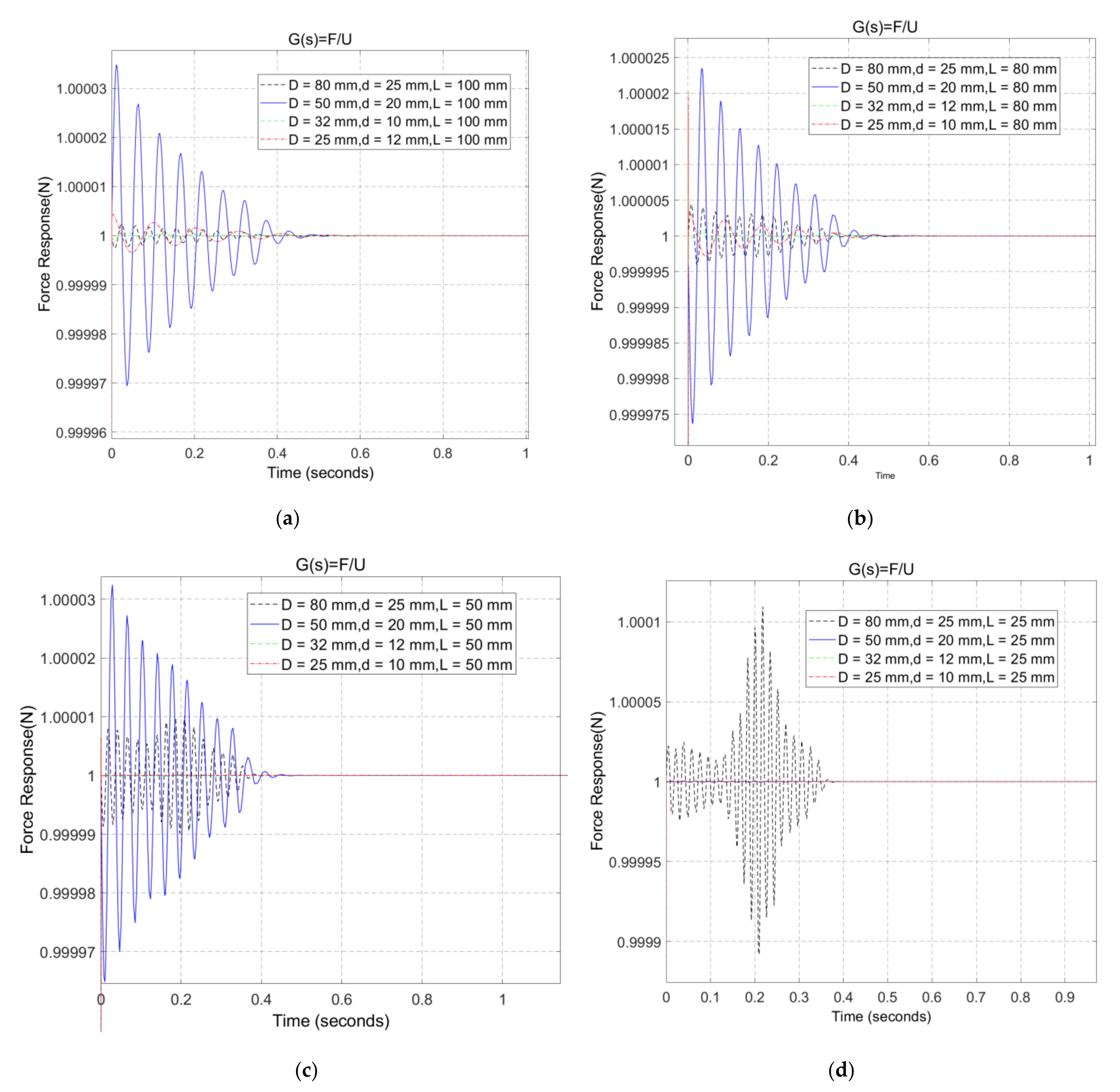
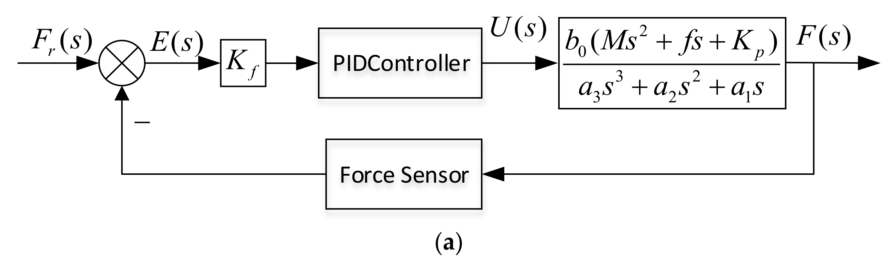
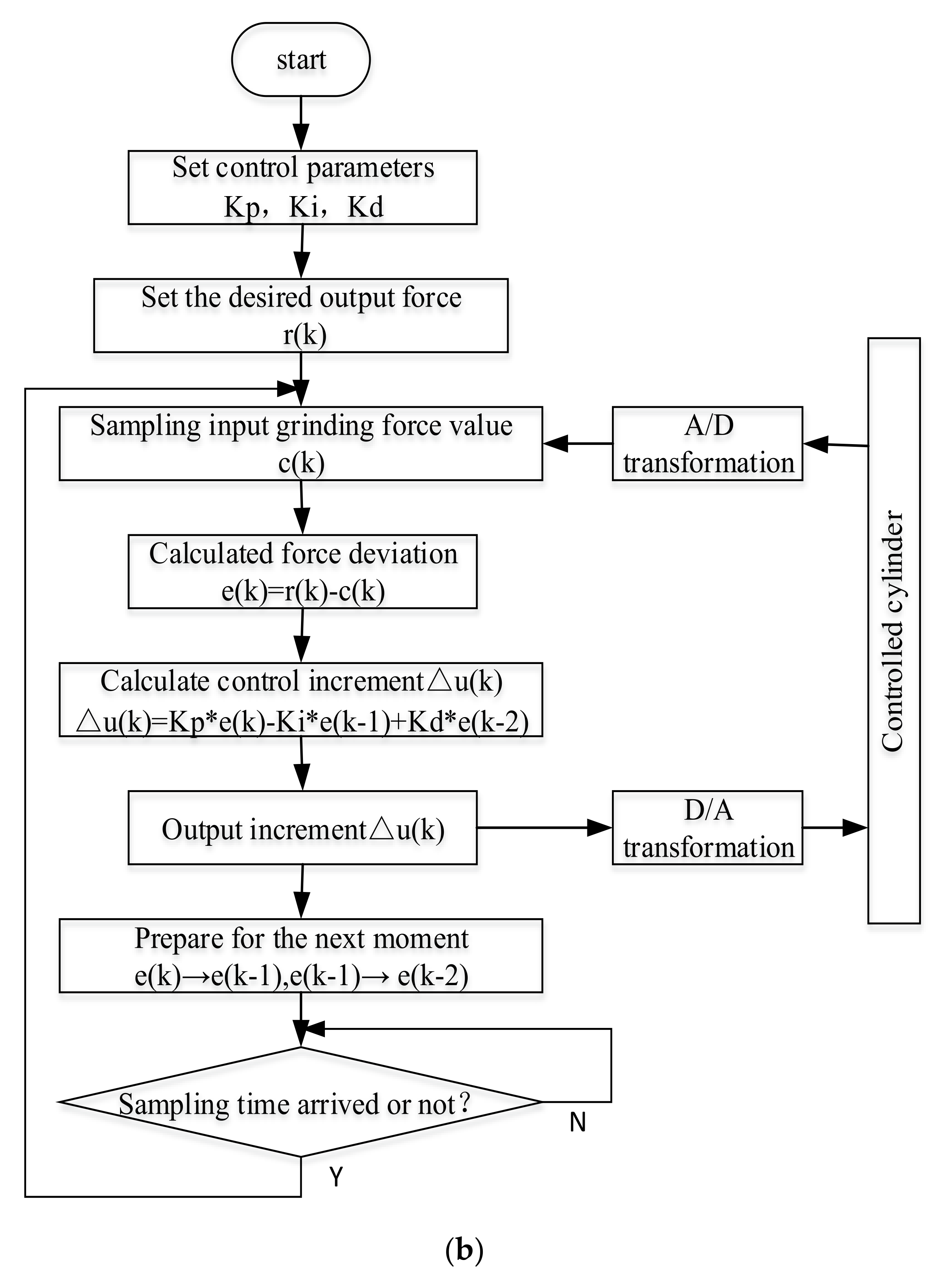
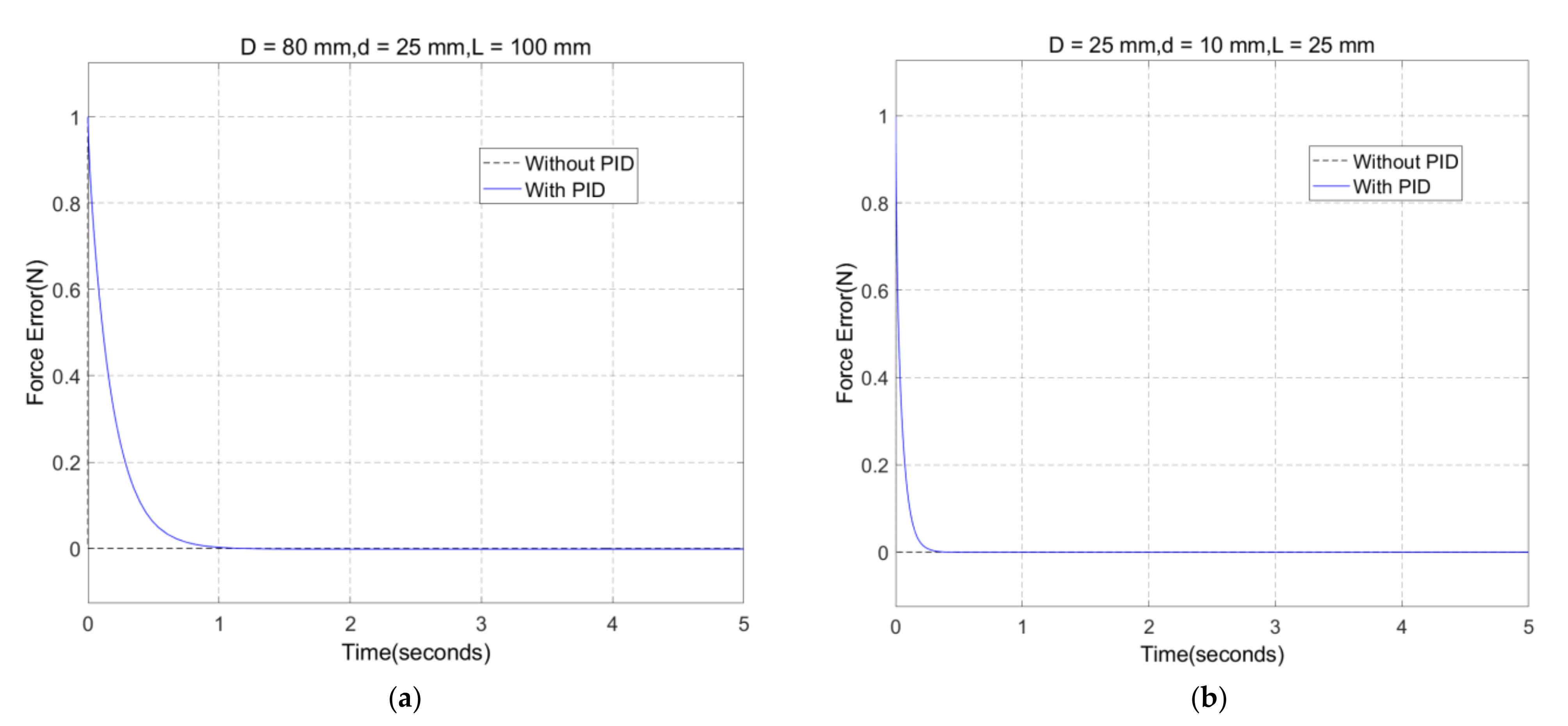
6.2. Force Response PID Correction and Control of Pneumatic Servo System

Since the output force of the pneumatic servo system has the problem of impact and oscillation in the initial stage, in order to improve the force control performance and reduce the impact and oscillation, the PID controller was introduced to correct and adjust the system. The system control block diagram and flow diagram are shown in Figure 15; Figure 15a shows the block diagram of a PID control system and Figure 15b shows the flow chart of a PID control system.

The force response curves of PID control based on force feedback are shown in Figure 16 and Figure 17. Figure 16 shows the response curves of the PID control force with the same cylinder diameter and different strokes. Figure 16 shows that under the same PID parameters, the larger the stroke, the longer the time taken to reach stability. Figure 17 shows the force response curves of PID control with the same stroke and different cylinder diameters and different piston rod. In Figure 17a,b, the PID parameters are the same, namely Kp = 1 × 10⁻⁴, Ki = 1 × 10⁻⁶, Kd = 1 × 10⁻⁶. Figure 17a,b shows that under the same PID parameters, the time taken for the force response to reach stability is not affected by the cylinder diameter. In Figure 17c,d, the PID parameters are Kp = 2 × 10⁻⁴, Ki = 1 × 10⁻⁶, Kd = 1 × 10⁻⁵ when the cylinder diameter D = 80 mm and the piston rod diameter d = 25 mm; the other PID parameters are the same, namely Kp = 1 × 10⁻⁴, Ki = 1 × 10⁻⁶, Kd = 1 × 10⁻⁶. Figure 17c,d show that under the same PID parameters, the time taken for the force response to reach stability is not affected by the cylinder diameter, except that the cylinder diameter D = 80 mm and the piston rod diameter d = 25 mm. Figure 18 shows force error curves before and after PID correction when the cylinder diameter D = 80 mm the piston rod diameter d = 25 mm, and the stroke L = 100, and when the cylinder diameter D = 25 mm, the piston rod diameter d = 10 mm, and the stroke L = 25, respectively. The average steady-state errors are shown in

Table 4. The average steady-state errors.

Cylinder Parameters	Error without PID	Error with PID
D = 80 mm, d = 25 mm, L = 100 mm	1.40 × 10−13%	0.042%
D = 25 mm, d = 10 mm, L = 25 mm	1.33 × 10−11%	0.141%

, illustrating that the pneumatic servo system has adequate stability in force control. In summary, the use of the PID control algorithm can overcome the impact and oscillation in the initial stage, thus improving the stability of the force control system.

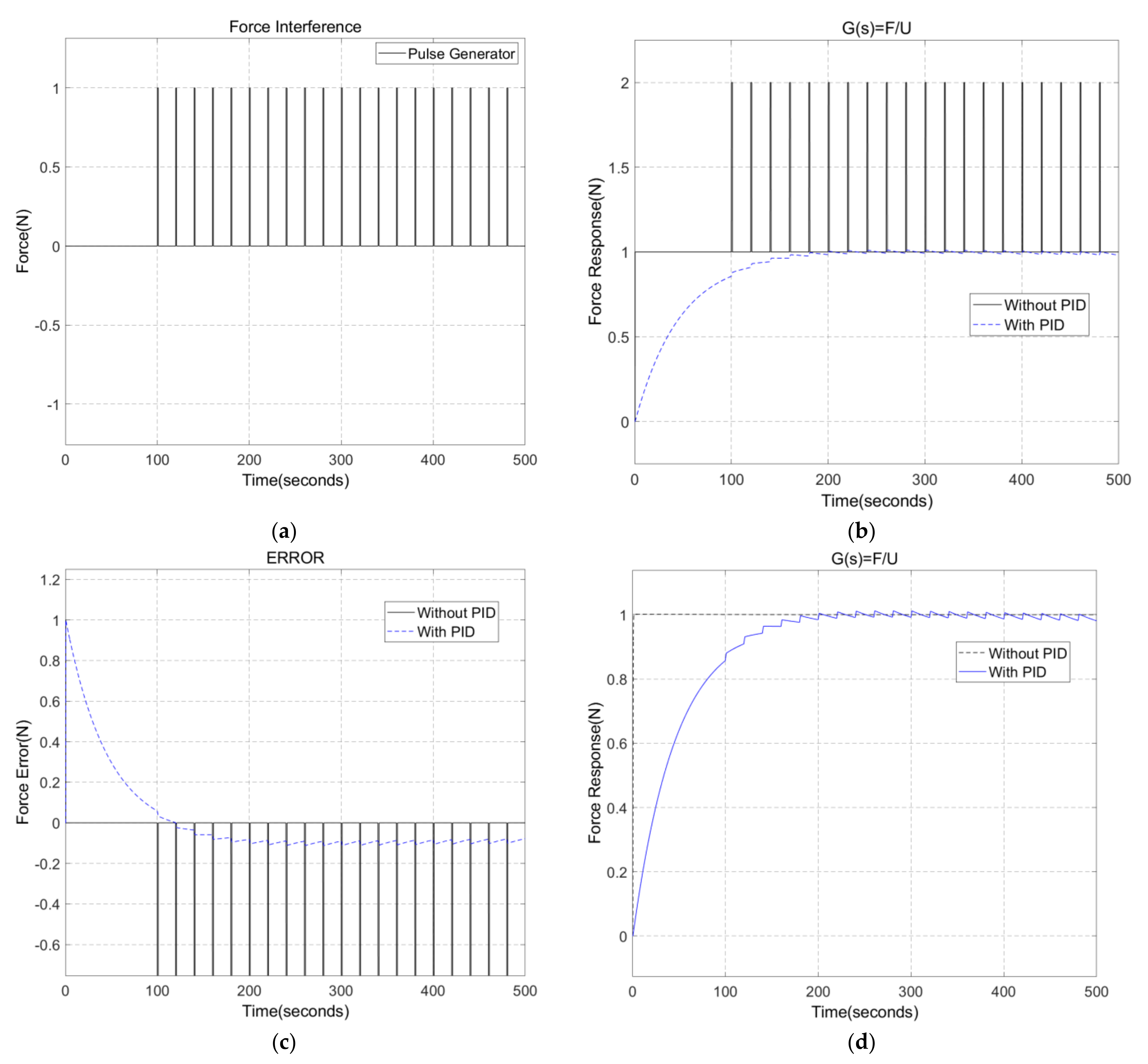
6.3. Grinding Force Control under Interference

In the practical application process, the system can be affected by various interference signals. In the grinding process, pulse interference signals are set to analyze the constant force characteristics of the pneumatic servo system. Take the cylinders with cylinder diameter D = 80 mm, piston rod diameter d = 25 mm, and stroke L = 100 mm as examples for analysis. Figure 19a shows the interference signal and the set pulse jamming signal parameters are amplitude = 1, period = 20 s, pulse width = 5% of period, and phase delay = 100 s. Figure 19b shows the force response curves with and without PID controller. It can be seen in Figure 19b that the influence of interference signals can be effectively suppressed by adopting PID control so that the system realizes constant force control. Figure 19c shows the error curve with or without PID control, and that the average steady-state error decreased from 5.95% to 0.785%. Figure 19d shows the force response curve with and without interference. It can be seen from the comparison that it takes longer to reach stability when there is interference. From 2.5 s to 200 s, PID can suppress the influence of interference well, but the time cost is higher, and there are still small sawtooth fluctuations. To further improve the constant force control performance, an intelligent control algorithm must be used for optimization.

7. Conclusions

In this paper, we studied the compliance of the grinding robot with the inner circle of the centrifugal pump shell. The macro–micro manipulator structure was adopted, the industrial manipulator realized the position control, and the pneumatic servo system was adopted for controlling the contact force in the grinding process with the end actuator. At the same time, the compressibility of gas was used to realize the compliance of the end effector. The relationship between the constant force control performance of the end effector and the structural parameters of the cylinder was analyzed in detail. The PID control algorithm was used to realize the fast response and stable control of the displacement and force output of the pneumatic servo system. The corresponding relationship between the PID gain and the structural parameters of the cylinder was obtained to carry out the simulation experiment. The simulation results show that the PID control improved the response speed and steady-state accuracy of the system, reduced the impact and oscillation of the system contact force, and effectively suppressed the influence of load interference, so that the average steady-state error decreased from 5.95% to 0.785%. The average steady-state error with load interference is 0.785% and the steady-state error without interference is 0.042% when the cylinder diameter D = 80 mm, the piston rod diameter d = 25 mm, and the stroke L = 100 mm with PID control. It realized the constant control of the contact force in the robot grinding process, so as to realize the stable, accurate, and fast response control of the grinding force. The uncertainty and complexity of force control in the grinding process of an industrial robot were resolved. The control strategy proposed in this paper is based on a simplified mathematical model of the pneumatic servo system. In the derivation process, it was assumed that the gas is ideal and the working pressure of the cylinder is constant. Therefore, the mathematical model established in this paper has certain limitations. Using intelligent control algorithms to study the constant force control of robots in the presence of interference, achieving the self-adaptive adjustment of control parameters, and verifying constant force control through experiments will be the focus of a future study.

References

1. Kalt, E.; Monfared, R.; Jackson, M. Towards an automated polishing system—Capturing manual polishing operations. Int. J. Res. Eng. Technol. 2016, 5, 182–192. [Google Scholar]
2. Huang, H.; Zhou, L.; Chen, X.; Gong, Z. Smart robotic system for 3d profile turbine vane airfoil repair. Int. J. Adv. Manuf. Technol. 2003, 21, 275–283. [Google Scholar] [CrossRef]
3. Mohammad, A.E.K.; Wang, D. A novel mechatronics design of an electrochemical mechanical end-effector for robotic-based surface polishing. In Proceedings of the 2015 IEEE/SICE International Symposium on System Integration (SII), Nagoya, Japan, 11–13 December 2015; pp. 127–133. [Google Scholar] [CrossRef]
4. Wang, T.; Miao, H.; Shi, S.; Chen, Z.; Zhang, H. A Method of Robot Grinding Force Control Based on Internal Model Control Principle. J. Phys. Conf. Ser. 2021, 1748, 1–5. [Google Scholar] [CrossRef]
5. Zhou, H.; Ma, S.; Wang, G.; Deng, Y.; Liu, Z. A Hybrid Control Strategy for Grinding and Polishing Robot Based on Adaptive Impedance Control. Adv. Mech. Eng. 2021, 13, 1–21. [Google Scholar] [CrossRef]
6. Jinno, M.; Ozaki, F.; Yoshimi, T.; Tatsuno, K.; Takahashi, M.; Kanda, M.; Tamada, Y.; Nagataki, S. Development of a Force Controlled Robot for Grinding, Chamfering and Polishi. In Proceedings of the 1995 IEEE International Conference on Robotics and Automation, Nagoya, Japan, 21–27 May 1995; pp. 1455–1460. [Google Scholar]
7. Tahvilian, A.M.; Hazel, B.; Rafieian, F.; Liu, Z.; Champliaud, H. Force Model for Impact Cutting Grinding with a Flexible Robotic Tool Holder. Int. J. Adv. Manuf. Technol. 2015, 85, 133–147. [Google Scholar] [CrossRef]
8. Wang, F.; Luo, Z.; Liu, H. Rapid Modelling and Grinding of Workpieces’ Inner-surface by Robot with Impedance Model Based Fuzzy Force Control Algorithm. MATEC Web Conf. 2017, 95, 05003. [Google Scholar] [CrossRef]
9. Attiya, A.J.; Wenyu, Y.; Shneen, S.W. Fuzzy-PID Controller of Robotic Grinding Force Servo System. TELKOMNIKA 2015, 15, 87–99. [Google Scholar] [CrossRef]
10. Xie, Y.; Yang, J.; Feng, M.; Huang, W.; Li, J. Path planning of grinding robot with force control based on B-spline curve. In Proceedings of the 2019 IEEE International Conference on Robotics and Biomimetics (ROBIO), Dali, China, 6–8 December 2019; pp. 2732–2736. [Google Scholar]
11. Zhang, T.; Xiao, M.; Zou, Y.; Xiao, J. Robotic Constant-force Grinding Control with a Press-and-release Model and Model-based Reinforcement Learning. Int. J. Adv. Manuf. Technol. 2019, 106, 589–602. [Google Scholar] [CrossRef]
12. Zhou, P.; Zhou, Y.; Xie, Q.; Zhao, H. Adaptive Force Control for Robotic Grinding of Complex Blades. In Proceedings of the 2019 5th International Conference on Mechanical Engineering and Automation Science (ICMEAS 2019), Wuhan, China, 10–12 October 2019; IOP Publishing: Bristol, UK, 2019; pp. 66–73. [Google Scholar]
13. Attiya, A.J.; Wenyu, Y.; Shneen, S.W. PSO_PI Controller of Robotic Grinding Force Servo System. TELKOMNIKA Indones. J. Electr. Eng. 2015, 15, 515–525. [Google Scholar] [CrossRef]
14. Zhang, T.; Yu, Y.; Yang, L.X.; Xiao, M.; Chen, S.Y. Robot Grinding System Trajectory Compensation Based on Co-kriging Method and constant-force Control Based on Adaptive Iterative Algorithm. Int. J. Precis. Eng. Manuf. 2020, 21, 1637–1651. [Google Scholar] [CrossRef]
15. Xiao, M.; Zhang, T.; Zou, Y.; Chen, S. Robotic constant force grinding control based on grinding model and model and model-based reinforcement learning. Ind. Robot. Int. J. Robot. Res. Appl. 2021, 48, 270–279. [Google Scholar] [CrossRef]
16. Sun, L. Research on Contact Force Control of Grinding Robot Based on Adaptive Impedance Control. In Proceedings of the 2021 IEEE 5th Information Technology, Networking, Electronic and Automation Control Conference (ITNEC), Xi’an, China, 15–17 October 2021; pp. 290–293. [Google Scholar]
17. Wang, Z.; Zou, L.; Luo, G.; Lv, C.; Huang, Y. A novel selected force controlling method for improving robotic grinding accuracy of complex curved blade. ISA Trans. 2022. [Google Scholar] [CrossRef]
18. Husmann, S.; Stemmler, S.; Hähnel, S.; Vogelgesang, S.; Abel, D.; Bergs, T. Model Predictive Force Control in Grinding Based on a Lightweight Robot. IFAC 2019, 52, 1779–1784. [Google Scholar] [CrossRef]
19. Zhu, D.; Feng, X.; Xu, X.; Yang, Z.; Li, W.; Yan, S.; Ding, H. Robotic Grinding of Complex Components a Step Towards Efficient and Intelligent Machining-Challenges, Solutions, and Applications. Robot. Comput. Integr. Manuf. 2020, 65, 10198. [Google Scholar] [CrossRef]
20. Wang, N.; Chen, C.; Di Nuovo, A. A Framework of Hybrid Force_Motion Skills Learning for Robots. IEEE Trans. Cogn. Dev. Syst. 2021, 13, 162–170. [Google Scholar] [CrossRef]
21. Wang, Q.; Wang, W.; Zheng, L.; Yun, C. Force control-based vibration suppression in robotic grinding of large thin-wall shells. Robot. Comput.-Integr. Manuf. 2021, 67, 102031. [Google Scholar] [CrossRef]
22. Ma, Z.; Huang, P. Adaptive Neural-Network Controller for an Uncertain Rigid Manipulator with Input Saturation and Full-Order State Constraint. IEEE Trans. Cybern. 2022, 52, 2907–2915. [Google Scholar] [CrossRef]
23. Xu, X.; Chen, W.; Zhu, D.; Yan, S.; Ding, H. Hybrid active_passive force control strategy for grinding marks suppression and profile accuracy enhancement in robotic belt grinding of turbine blade. Robot. Comput. -Integr. Manuf. 2021, 67, 102047. [Google Scholar] [CrossRef]
24. Xu, Z.; Li, S.; Zhou, X.; Zhou, S.; Cheng, T.; Guan, Y. Dynamic Neural Networks for Motion-Force Control of Redundant Manipulators_ An Optimization Perspective. IEEE Trans. Ind. Electron. 2021, 68, 1525–1536. [Google Scholar] [CrossRef]
25. Tian, F.; Lv, C.; Li, Z.; Liu, G. Modeling and control of robotic automatic polishing for curved. CIRP J. Manuf. Sci. Technol. 2016, 14, 55–64. [Google Scholar] [CrossRef]
26. Khoi, P.B.; Hai, H.T.; Sinh, H.V. Dynamic analysis of robot in machining. Int. J. Mech. Prod. Eng. Res. Dev. 2020, 10, 223–236. [Google Scholar]
27. Senoo, T.; Koike, M.; Murakami, K.; Ishikawa, M. Impedance Control Design Based on Plastic Deformation for a Robotic Arm. IEEE Robot. Autom. Lett. 2016, 2, 209–216. [Google Scholar] [CrossRef]
28. Chaudhary, H.; Panwar, V.; Prasad, R.; Sukavanam, N. Adaptive neuro fuzzy based hybrid force/position control for an industrial robot manipulator. J. Intell. Manuf. 2016, 27, 1299–1308. [Google Scholar] [CrossRef]
29. Cavenago, F.; Giordano, A.M.; Massari, M. Contact force observer for space robots. In Proceedings of the 2019 IEEE 58th Conference on Decision and Control (CDC), Nice, France, 11–13 December 2019; pp. 2528–2535. [Google Scholar]
30. Takeuchi, Y.; Ge, D.; Asakawa, N. Automated polishing process with a human-like dexterous robot. In Proceedings of the IEEE International Conference on Robotics & Automation, Atlanta, GA, USA, 2–6 May 1993. [Google Scholar]
31. Asada, H.; Goldfine, N. Optimal compliance design for grinding robot tool holders. In Proceedings of the IEEE International Conference on Robotics & Automation, St. Louis, MO, USA, 25–28 March 1985. [Google Scholar]
32. Takeuchi, Y.; Asakawa, N.; Ge, D. Automation of Polishing Work by an Industrial Robot: System of Polishing Robot. JSME Int. J. 1993, 36, 56–561. [Google Scholar] [CrossRef]
33. Chen, Z. Calculation and Application of Internal Grinding Force. Grinder Grind. 1991, 45–46, 81. [Google Scholar] [CrossRef]
34. Bai, Y. Pneumatic Servo System Analysis and Control; Metallurgical Industry Press: Beijing, China, 2014. [Google Scholar]
35. Sanville, F.E. A new method of specifying the flow capacity of pneumatic fluid valves. Hydraul. Pneum. Power 1971, 17, 120–125. [Google Scholar]
Figure 1. Force analysis diagram of internal grinding.
Applsci 12 09708 g001
Figure 2. Three-dimensional model of the grinding system. (a) Layout of grinding system, (b) Grinding device.
Applsci 12 09708 g002aApplsci 12 09708 g002b
Figure 3. Block diagram of the pneumatic control system of the robot grinding and polishing device.
Applsci 12 09708 g003
Figure 4. Schematic diagram of the pneumatic control based on the VER servo valve.
Applsci 12 09708 g004
Figure 5. Block diagram of the open-loop transfer function of the pneumatic servo system.
Applsci 12 09708 g005
Figure 6. Block diagram of the closed-loop system of the pneumatic servo system.
Applsci 12 09708 g006
Figure 7. Response curves of different stroke positions. (a) D = 80 mm, d = 25 mm; (b) D = 50 mm, d = 20 mm; (c) D = 32 mm, d = 12 mm; (d) D = 25 mm, d = 10 mm.
Applsci 12 09708 g007
Figure 8. Output response curves of cylinder positions with different cylinder diameters. (a) L = 100 mm; (b) L = 80 mm; (c) L = 50 mm; (d) L = 25 mm.
Applsci 12 09708 g008
Figure 9. Response curves of the output force at different strokes. (a) D = 80 mm, d = 25 mm; (b) D = 50 mm, d = 25 mm (partial enlarged view at the initial stage); (c) D = 50 mm, d = 20 mm; (d) D = 50 mm, d = 20 mm (partial enlarged view at the initial stage); (e) D = 32 mm, d = 12 mm; (f) D = 32 mm, d = 12 mm (partial enlarged view at the initial stage); (g) D = 25 mm, d = 10 mm; (h) D = 25 mm, d = 10 mm (partial enlarged view at the initial stage).
Applsci 12 09708 g009aApplsci 12 09708 g009b
Figure 10. Output force response curves of different cylinder diameters. (a) L = 100 mm; (b) L = 80 mm; (c) L = 50 mm; (d) L = 25 mm.
Applsci 12 09708 g010
Figure 11. Block diagram of the feedback control system.
Applsci 12 09708 g011
Figure 12. Block diagram of the displacement and acceleration feedback control.
Applsci 12 09708 g012
Figure 13. Response curves of different stroke positions. (a) Kp = 5, Ki = 1 × 10⁻⁹, Kd = 1 × 10⁶; (b) Kp = 3, Ki = 1 × 10⁻⁹, Kd = 1 × 10 6; (c) Kp = 0.9, Ki = 1 × 10⁻⁹, Kd = 1 × 10⁶; (d) Kp = 0.9, Ki = 1 × 10⁻⁹, Kd = 1 × 10⁶.
Applsci 12 09708 g013
Figure 14. Response curves of different cylinder bore positions. (a) L = 100 mm; (b) L = 80 mm; (c) L = 50 mm; (d) L = 25 mm.
Applsci 12 09708 g014aApplsci 12 09708 g014b
Figure 15. Diagram of a PID control system. (a) Block diagram of a PID control system; (b) Flow chart of a PID control system.
Applsci 12 09708 g015aApplsci 12 09708 g015b
Figure 16. Force response curves with the same cylinder diameter and different strokes. (a) D = 80 mm, Kp = 1 × 10⁻⁴, Ki = 1 × 10⁻⁶, Kd = 1 × 10⁻⁶; (b) D = 50 mm, Kp = 1 × 10⁻⁴, Ki = 1 × 10⁻⁶, Kd = 1 × 10⁻⁶; (c) D = 32 mm, Kp = 1 × 10⁻⁴, Ki = 1 × 10⁻⁶, Kd = 1 × 10⁻⁶; (d) D = 25 mm, Kp = 1 × 10⁻⁴, Ki = 1 × 10⁻⁶, Kd = 1 × 10⁻⁶.
Applsci 12 09708 g016
Figure 17. Force response curves with different cylinder diameters and the same stroke. (a) L = 100 mm; (b) L = 80 mm; (c) L = 50 mm; (d) L = 25 mm.
Applsci 12 09708 g017
Figure 18. Force error curves before and after PID correction. (a) D = 80 mm, d = 25 mm, L = 100 mm; (b) D = 25 mm, d = 10 mm, L = 25 mm.
Applsci 12 09708 g018
Figure 19. Force response curves with interference. (a) Interference signal; (b) Force response curves with interference; (c) Error curves with and without PID control; (d) Comparison of PID control response curves with and without interference.
Applsci 12 09708 g019