Measurement-Driven Synthesis of Female Digital Mannequin Using Convex Sub-Volumes

Abstract

In the context of computer-aided apparel-fitting simulation, the problem of generating (a) simulation-inexpensive and (b) tailor-measurement-driven digital mannequins is central. Three-dimensional scanning of human bodies produces high-fidelity datasets. However, this technique does not satisfy conditions (a) and (b) above. In addition, it requires extensive data cleaning and processing. Existing approaches to this problem broadly fall into these mainstreams: (i) biased scaling, interpolation, or morphing of template models; or (ii) bottom-up construction of anatomy (bone medial axis, kinematic joints, muscles, skin, and other layers). Both alternatives imply extensive scanning, application of heuristics, tuning, and storage, among other tasks. Both alternatives produce non-convex datasets that have to be processed further for cloth–body interaction simulation, as physics engines require some type of data convexity for realistic simulations. This manuscript presents a modeling methodology that partially overcomes these limitations by (1) coarsely approximating a template female body with sets of convex volumes (ellipsoids and cushions), (2) building a set of Reference Mannequins for a particular set of extreme and average tailor measurements, and (3) creating sets of functions that synthesize new individuals of digital mannequins as reunions of convex volumes that satisfy specified tailor measurements. These mannequins present a reasonable and realistic demeanor. At the same time, they are shown to be economical at the stage of simulation of garment fitting. Future work is encouraged to define kinematic chains for straightforward pose definition, modeling male bodies, and exploring the behavior of the synthesis functions with more parameters.

1. Introduction

1.1. Context

Parametric modeling of the human body (in the relevant literature [1,2]) is the process by which 3D digital representations of diverse body shapes and sizes can be synthesized from input measurements and example models. An advantage of parametric human body modeling is the possibility of economically and flexibly avoiding scanning or manual digital sculpting to obtain 3D models of different phenotypes [1]. Parametric modeling of humans is applied in virtual tailoring, garment fitting simulation, human motion modeling, avatar creation, character design, etc.

Digital mannequin realization and virtual garment trial directly implement physics and mathematical theories and tools (statistics, differential geometry and equations, signal processing, kinematics, multi-particle systems, thin-plate energy, strain modeling, etc.). Time optimization in these fields touches topics such as scalar and vector fields, hash functions, lattice geometry, topology, etc. Garment fitting [3,4] and mannequin modeling [1] rely heavily on computational geometry and topology tools.

Usual parametric modeling produces mappings between body surface point clouds and anthropometric (i.e., tailor) measurements. A goal is to produce new point clouds that obey extended sets of tailor measurements. Prescribing the position of massive amounts of points by using analytical forms or constraints easily produces unnatural, illegal, self-intersecting, or non-manifold meshes or point clouds. Additional tuning and processing are then required. In point-cloud-based modeling, execution time and storage expenses are very large.

1.2. Research Strategy and Scope

This manuscript applies to digital model synthesis, the well-known practice in the artistic drawing and sketching domain of approximating a human or animal body by a set of ellipsoids. This set of ellipsoidal primitives effectively captures the pose and demeanor of the (static) female model. It does not concern itself with the details. A bijective mapping tailor measurements vs. ellipsoid set is computed. This mapping allows the synthesis of a female mannequin that satisfies a set of tailor measurements. It also allows extraction of the tailor measurements of a given mannequin. We then use a derivative convex primitive, called cushion (the convex hull of two ellipsoids), to complement the approximation of the female human body. We do not seek to arrive at a mesh representation of the body. Therefore, our approach does not incur the expenses of mesh cleaning, repairing, convex decomposition, etc. The approximation of the female mannequin by using a set of convex primitives is accepted by some physics engines (e.g., [5]) to simulate garment–body interaction. Notice that we do not, in this manuscript, model garment–body interaction.

Our manuscript does not attempt the automated synthesis of digital mannequins from images, videos, or point clouds (neither static nor dynamic) through feature extractions and scalings, among other procedures. Our manuscript does not address mannequin kinetics or motion, nor recognition/classification of subject actions or activities. For readers interested in these topics, references [6,7] may provide useful insight. The interest of our effort is to use a convex primitive approximation of a digital mannequin and tailor measurements in order to create other digital individuals with diverse sizes. Our manuscript executes interpolation among sizes of ellipsoid-based mannequins by finding and using bijections between sets of tailor measurements and ellipsoid-based mannequins. Our manuscript addresses static (as opposed to motion) scenarios.

Our industrial sponsor has female mannequins and garments as its priority. This fact explains why this publication does not address male digital mannequins. Future efforts will do so.

The problem that this manuscript addresses is formulated as:

Given

• $Me$: A set of measurements $Me=[He,Sh,Br,Wa,Hi]$ that describe the shape of a female body. With $He$: Height, $Sh$: Shoulder width, $Br$: Breast perimeter, $Wa$: Waist perimeter, and $Hi$: Hip perimeter.

Goal

• B: 3D mannequin approximation of a female body that satisfies a particular set of tailor measurements $Me$. B is a set of convex volumes.

1.3. Manuscript Structure

This manuscript is structured as follows: Section 2 reviews the existing literature, drawing conclusions to justify the manuscript. Section 3 explains the methodology followed to model and synthesize the mannequins. Section 4 presents the results of our method and a particular application to demonstrate its usefulness. Section 5 concludes the manuscript and discusses relevant future endeavors.

2. Literature Review

The current literature for parametric modeling can be divided into two main categories: (i) non-convex example-based modeling through scalings and morphings, and (ii) bottom-up construction of anatomy-based models (bone medial axis, joints, muscles, and skin). This section seeks to give a taxonomy and summary of the current methods found in the literature, as well as to expand on the different approaches found for both categories.

2.1. Non-Convex Example-Based Modeling

The most common approach found in the literature for the parametric modeling of human bodies is non-convex example-based modeling. For this general approach, researchers mainly extract features (e.g., cross sections, anatomical landmarks, and patches) from 3D-scanned point-clouds, digital template models, or images. Afterwards, they determine the relation between measurements and features in order to either deform a template model or interpolate multiple examples.

In general, these approaches present the following limitations: (1) The synthesized model is a non-convex mesh or point-cloud. (2) The resulting model needs further processing to be used for simulations concerning collision detection. (3) They requires the use of expensive algorithms for feature extraction, deformation, ensuring surface continuity, and surface-fitting. (4) Re-computation/deformation of non-convex surfaces is needed in order to define new poses. (5) This method is dependent on hardware and/or a large database of examples. A summary of the different approaches found for this particular category is presented next, where each particular reference is discussed in further detail.

2.1.1. Deformation of a Single Template/Example Model

References [8,9,10,11,12,13,14,15,16] extract features from a single digital template model or 3D scan and apply deformation functions in order to synthesize variations that satisfy input measurements.

• Reference [8] imposes symmetric constraints to the ‘SCAPE’ parametric model. These symmetric constraints are defined as symmetry-related matrices and are applied during pose and shape deformation to provide a resulting symmetric model.
• Reference [9] proposes a tensor decomposition technique to model human bodies based on data (shape and pose) of multiple subjects. They use such data to train a deformation method that considers pose and shape parameters in conjunction rather than independently. This method is applied to a template model.
• Reference [10] proposes the segmentation of a template model (point-cloud) into regular intervals. These intervals are subsets of point-clouds to which shape control lines (SCL) are fitted. The SCLs are then modified by applying centroid-based and ratio-based scalings to produce variations of the template.
• Reference [11] extracts contour (features) from a scanned model. These contours are measured and translated vertically according to the template model’s height and the input height. The shape of the scanned model is then modified by applying linear anthropometric rules to produce an adaptive mannequin.
• Reference [12] extracts shape and measurement information from a template model. The authors identify key parameters that define the scaling for the global deformation (responsible for general shape) and feature factors for local deformation (of specific parts of the body). Nonlinear interpolation is used to deform the overall shape and critical parts of the template model based on the key parameters.
• Reference [13] extracts cross sections from a scanned dataset of a physical mannequin. The initial locations of the cross sections are obtained using statistical anthropometric data. These cross sections are deformed by resizing and relocating according to input anthropometric data (measurements) that describes the desired geometry.
• Reference [14] extracts cross sections and characteristic points (features) from a template model. Then, characteristic sizes are calculated (heights and circumferences) based on the features. Nineteen main control points are established and used to perform a three-dimensional lengthwise axial deformation. Radial deformation is used to perform girth-wise or area deformations.
• Reference [15] obtains parameter-to-geometry correlations by using radial-basis interpolation over a number of 3D scanned models. These correlations allow for the creation of deformation functions. A template model is then deformed through skeletal deformation, and geometric and energy-based processes are used to calculate vertex displacement.
• Reference [16] performs a manual segmentation of a template model and applies spline and radial-basis deformation functions and continuity filters to change the shape and size of the template model.

2.1.2. Synthesis through Multiple Example Models

References [2,17,18,19,20,21,22,23,24,25] extract features from sets of 3D scans of different individuals and correlate their variations in size and shape to each of their measurements. With such correlation, new individuals can be produced based on input measurements.

• Reference [2] proposes the creation of a database from scanned models. Correlations between the meshes (feature points and curves) and semantic parameters are created and computed as a linear system of equations. The system of equations has its complexity reduced through PCA. New models are produced by modifying input models or finding and modifying similar models (from databases) to satisfy input measurements.
• References [17,18] preprocess 250 (125 females and 125 males) scanned models from the SizeKorea database. The models are categorized, and the correlations between body shape variation and body sizes are extracted through statistical analysis (PCA). With such correlations, new models are obtained through shape parameter optimization techniques and radial-basis function (RBF) deformation of a template surface.
• Reference [19] obtains a set of thousands of scans, for which they extract and correct landmarks. Then, PCA is performed to extract the parameters that define shape variation, which are stored in a database. Moreover, a system in which users can have access to individual 3D scanned data and personalized body-shape modeling is presented.
• Reference [20] presents a unified model that describes pose, shape, and muscular deformation. A set of 550 full-body scans of 114 subjects is obtained, registered, and encoded. Rotation-invariant encoding allows for the creation of semantic regression functions (PCA-based technique). The regression functions are used to generate arbitrary models.
• Reference [21] constructs a database of 160 (80 male and 80 female) body scans. PCA is then performed to parameterize the data and characterize the tendency of shape variation and modeling parameters, and their correlation with anthropometric parameters. Through such correlations and a non-linear error-optimization-based shape modeling method, an arbitrary model can be obtained from user-specified measurements.
• Reference [22] extracts feature points from a set of scanned models. The feature points are used to create feature curves, which are then parameterized. Using a numerical optimization-based scheme, a new model can be synthesized by interpolating certain examples from the database. These examples are selected through an optimization algorithm.
• Reference [23] proposes a learning-based method to define the relationship between feature curves (wireframes) and anthropometric measurements. Such a relationship is built using a deep neural network (DNN) based on a test dataset and used to build new wireframes. New meshes can be created by interpolating the new wireframes into patches.
• Reference [24] proposes a modeling scheme called SMPL, which uses 2100 female models from the CAESAR project database to train a set of parameters. Such parameters are used in linear blending functions (i.e., shape, skinning, and pose) and a regressor to reconstruct a new mesh from the vertex of a template mesh.
• Reference [25] proposes the extraction of measurements from 1024 bodies using VR controllers (i.e., HTC Vive). These measurements are then related to the SIMPL [24] model shape parameters. With such relations, the author train four regressors that allow the creation of new meshes from body measurements obtained with the VR controllers.

2.1.3. Feature Extraction from Photographs

References [26,27,28,29,30,31,32] use photographs to extract silhouettes (features) and feature points that are used as references to deform and fit a template model, or to reconstruct a new model from the extracted features.

• Reference [26] captures orthogonal pictures of a person and extracts silhouettes. Feature points are obtained from the silhouettes and used to define a linear affine mapping of the correlation between the template model and the silhouettes. This mapping is then used to define and apply shape deformation to the 3D template model.
• Reference [27] manually defines feature points on three orthogonal pictures of a person. From the feature points, a silhouette is extracted and a skeleton is automatically fitted by applying affine transformations and Barycentric interpolation. A template model’s skin (surface) is then deformed through piecewise affine transformations and 2D-to-3D mapping with the skeleton and silhouette information.
• Reference [28] applies a segmentation method on two orthogonal photographs of a subject to extract contours (silhouettes). The silhouettes are correlated to silhouettes of a template model, and feature points are extracted using morphology rules and template-based feature extraction algorithms. The authors use the model and silhouette photographs to perform view-dependent deformation of the template model.
• Reference [29] presents a modeling scheme in which the authors deform a template model to best fit the user’s shape. The first step consists of fitting the template to a user-generated point-cloud via 3D scans and feature-point extraction. The second uses low-resolution 2D images to estimate the shape and pose of the human body, assisted by boundary constraints.
• Reference [30] presents a method for rebuilding 3D models based on a set of seven template models and orthographic images of a subject. The method consists of extracting contours from the images and scaling contours from the template models according to the extracted contours.
• Reference [31] estimates the 3D shape and pose of a subject from a single image. This process consists of regressing the 3D positions of the vertices of a SMPL-template mesh via graph convolutional networks, avoiding the use of anthropometric parameters.
• Reference [32] propose the reconstruction of 3D meshes from a single image. A graph convolutional network (GCN) is used to directly predict the 3D locations of mesh vertices from the input image. Anthropometric parameters are integrated into the GCN to improve the reconstruction accuracy.

2.2. Anatomy-Based Modeling

A particular family of approaches found in the literature consists of bottom-up manual modeling of individuals. These approaches focus on the influence of the pose over muscle deformation and its influence on the shape of the model (skin). They propose building a kinematic skeleton to which muscles and tissues are modeled and attached. Then, the shape of the muscles and tissues is parameterized as a function of the state of the kinematic joints. Finally, a surface-fitting procedure is performed to reproduce skin over the deformed muscles. These approaches present the following principal disadvantages: (1) A non-convex model is produced; (2) High computation expenses due to deformation algorithms and surface fitting with each change of state in the kinematic joints; (3) Modeling of multiple internal elements to reproduce external surfaces; (4) No possibility to synthesize different phenotypes from input measurements.

Reference [33] utilizes isotonic contraction and tension parameters to formulate muscle deformation. No skin approximation is presented. Reference [34] presents a scheme to approximate muscles as deformed cylinders that are parameterized to change size and shape with changes in joints. Skin is presented as an elastic surface that is deformed with changes in size and shape of the underlying components (tissue and muscle).

2.3. Conclusions of Literature Review

The main conclusions of the literature review are presented in this section with a summary exhibited in

Table 1. Comparison of previous approaches found in the literature plus our contribution.

Approach	Refs.	Advantages	Disadvantages
Non-Convex Example-Based Synthesis Approach	[2,8,9,10,11,12,13,14,15,16,18,19,20,21,22,23,24,25,26,27,28,29,30,31,32,35,36]	(1) Models with intricate details can be reproduced. (2) Continuity of mesh surface is achieved. (3) Anatomic fidelity of the model.	(1) A non-convex model is produced. (2) Needs further processing steps to generate a ready-to-simulate model. (3) Expensive algorithms for deformation and surface-fitting. (4) Pose limitation or need to recompute/deform surfaces for pose changes. (5) Dependent on hardware and/or a large database of examples.
Non-Convex Anatomy Based Approach: Bone, Muscle, Tissue Construction	[33,34]	(1) Anatomic fidelity of the model. (2) High kinematic fidelity can be achieved.	(1) A non-convex model is produced. (2) High computation expenses. (3) Construction of unnecessary internal elements to reproduce external surfaces. (4) Phenotype limitation.
Synthesis Based on Convex Volumes	Our approach	(1) Low computational costs. (2) No intermediate steps for the preparation of the model for physics simulation. (3) Simple and straightforward parameterization with minimal tuning. (4) Reduced storage of data. (5) No need of re-computations of surfaces to change poses.	(1) Low model resolution, leaving out intricate details of the body. (2) Model surface does not have $C^1$ surface continuity.

. This table exhibits a comparison between the advantages/disadvantages of previous schemes and of the approach presented in this manuscript. Such a comparison seeks to support the contributions made by the proposed approach.

In the current literature, the human body is modeled as non-convex meshes, with exceptions found in some components of the models produced by anatomy-based methods. These non-convex meshes are computationally expensive to process for pose variation and collision detection simulations (e.g., garment-fitting), among other implementations. In addition, example-based approaches present particular disadvantages in (1) requiring expensive hardware, (2) storage of large amounts of data, (3) usage of smoothing and surface-fitting algorithms, and (4) expensive extraction of features and identification of feature–parameter relations. It is also noted that anatomy-based approaches do not parameterize the general shape and size of the model. In contrast, they requires manual intervention for modeling a particular phenotype.

To overcome these limitations, this manuscript proposes a parametric modeling scheme based on convex volumes. The scheme synthesizes sets of convex volumes (mannequins) from sets of tailor measurements and a small set of manually created Reference Mannequins ($RM$). Furthermore, the synthesized models satisfy the input measurements. This approach presents the following contributions: (a) avoids the need for hardware and the storage of large amounts of data, (b) enables pose variation through kinematic chains without re-computing surfaces, (c) simple and straightforward parameterization with minimal tuning, and (d) the synthesized mannequins are ready-to-simulate and do not need further processing. In conclusion, to the best of our knowledge, no other approach based on convex volumes is found in the literature. Hence, our approach proves novel.

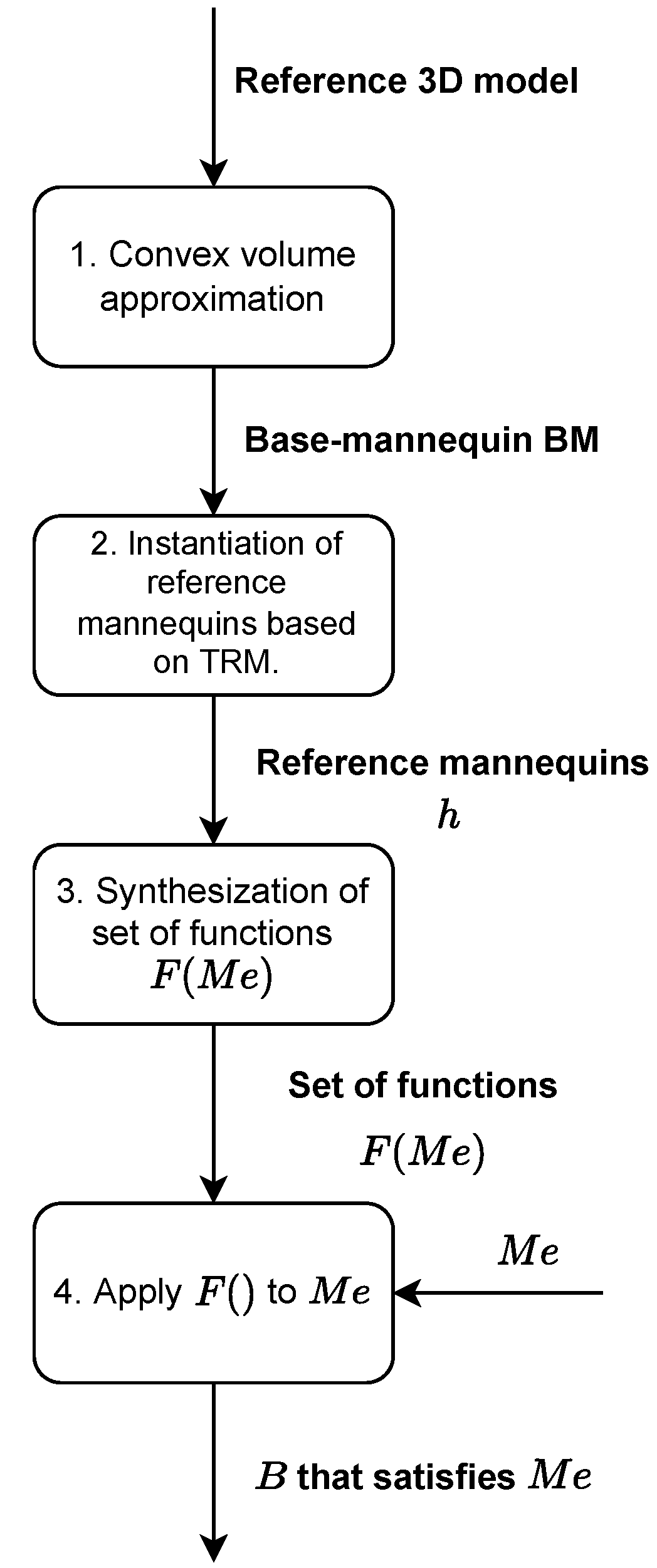
3. Materials and Methods

The proposed methodology consists of approximating a 3D model with convex volumes (ellipsoids and cushions), which we call a 3D mannequin. This mannequin is parameterized (synthesized as a function of tailor measurements) in order to obtain measurement-driven 3D mannequins. Such mannequins satisfy the desired measurements with a minimum margin of error. The main steps performed to produce the measurement-driven mannequins are as follows (see also Figure 1):

• A reference 3D model is manually approximated/traced with ellipsoids to produce a Base Mannequin ($BM$). Furthermore, an ellipsoid-to-cushion post-process is presented to improve the convex volume approximation after it has been parameterized. See Section 3.2.
• The $BM$ (set of ellipsoids) is then used to instance a set of Reference Mannequins ($RM$). Each one of these Reference Mannequins ($R{M}_i$) satisfies a particular set of five tailor measurements. See Section 3.3.
• Based on the known data of $RM$ (geometry and measurements), a set of functions $F\left(Me\right)$ is created. This set of functions synthesizes the geometry of a measurement-driven mannequin that in return satisfies the given measurements in $Me$. See Section 3.6.
• Finally, the measurement-driven mannequin can be synthesized by computing $F\left(Me\right)$.

Problem Specification

These steps are explained in more detail in the following subsections (see Section 3.2, Section 3.3 and Section 3.6). The problem of finding the parameterization for the 3D mannequins can be specified per the following given and goal:

Given:

• A: A set of points in ${\mathbb{R}}^q$. Each component j of a point x ($x\in A$), with $j=1,2,\cdots ,q$, represents a measurement of the human body in $Me$ (e.g., height, shoulder width, etc.). The following conditions must be considered:

  (a)

  $x_j>0,\forall j=1,2,\cdots ,q$.

  (b)

  L: A set of q ordered pairs corresponding to the lower and upper limits of the components j of x. $L:\left\{l\right|l_{1,2}>0,l_1<l_2\}$

• H: A set of sets of ellipsoids in ${\mathbb{R}}^3$. Each set of ellipsoids B, with $B\in H$, approximates the shape and size of a human body described by a point $x\in A$.

  (a)

  Each B has the same number m of ellipsoids and the same topology.

  (b)

  Each B satisfies the measurements of a specific point $x\in A$.

  (c)

  Each ellipsoid of B is defined by a homogeneous SO(3) coordinate system S and a triad D describing the dimensions of its semi-axes.

Goal:

• $m_T$: Function $m_T:H⟶A$; $m_T$ obtains the tailor measurements $Me$ of any model $B\in H$.
• F: A set of functions $F:A⟶H$, $F=m_T^{-1}$. More specifically, $F:x⟶B$, such that $m_T$ applied to $B=F\left(x\right)$ produces the measurements in x. F is a set of functions that, given a set of measurements x, synthesizes a model (geometry) B that satisfies x.

From Figure 1 it must be taken into consideration that Steps 1 through 3 are performed only once so as to produce F. The set of functions F is then computed each time a new mannequin is synthesized from defined measurements $Me$. It is also worth noting that the subject approximated by convex volumes in this manuscript is the female body. The same process could be applied to approximate the male body.

3.1. Rationale for the Mathematical Model

In order to obtain a parametric mannequin, a set of pre-processing and processing steps are carried out. The procedural enumerations and descriptions of these steps are addressed in Section 3.2–Section 3.4 for pre-processing and Section 3.5 and Section 3.6 for processing. The current subsection intends to highlight the main mathematical and scientific reasoning that provide support for such steps.

Geometrical and Topological Pre-Processing

Pre-processing seeks to facilitate the bijective mapping ellipsoid set ↔ tailor measurements by reducing (a) mathematical complexity and (b) numerical unstability. Pre-processing (1) manually constructs an ellipsoid set ($BM$) that approximates a mesh-based model, (2) reduces the degrees of freedom of the ellipsoid set, and (3) lowers the noise level within the ellipsoid set. Pre-processing consists of:

• Selection of ellipsoids due to their low geometrical complexity, low data-storage, and the benefits of convex volumes present in physics engines;
• Manual approximation of the 3D reference model by fitting a set of ellipsoids;
• Symmetrical location of ellipsoids with respect to the sagittal plane;
• Construction of a set of Reference Mannequins through rigid transformations of the set of ellipsoids;
• Compliance of Reference Mannequins to sets of tailor measurements;
• Data processing is performed over the set of Reference Mannequins in order to achieve:

  (a)

  Enforcement of symmetry with respect to the sagittal plane;

  (b)

  Enforcement of right-handedness in the ellipsoid coordinate systems;

  (c)

  Congruence of the coordinate system (definition of World Coordinate System);

  (d)

  Re-labeling of SO(3) coordinate systems (i.e., ellipsoid axes) to ensure minimal variation of the interpolation functions in set F.

By definition, our approach seeks large-scale (ellipsoid approximation) geometrical information of the mannequin. This scope filters out small details and noise. In this particular manuscript, such filtering was manually executed by fitting the ellipsoid set to the Base Mannequin. For this process to be executed in a semi-automated or automated manner, we suggest these topics: (a) alpha shape fitting [37] and (b) signal denoising [38].

Processing; Bijective Mapping; Tailor Measurements ↔ Ellipsoid Sets

Many possible sets of ellipsoids could satisfy the measurements of a particular $x\in A$, generating infinite $m_{T_i}^{-1}$. Therefore, a particular $F\subset m_T^{-1}$ has been selected, such that each $B=F\left(x\right)$ satisfies the measurements of an arbitrary x. F is then considered as the set of parametric functions that synthesizes a particular mannequin B given a desired set of measurements x and a set of known tuples of $RM$ (set of Reference Mannequins) containing geometry and measurements.

In addition to the previous precision made about the mapping from $x⟶B$, a set of reasonings is presented for the processing steps (interpolation method). These reasonings seek to avoid instability (erroneous sizing and unnatural demeanor) of the synthesized mannequins (see Section 3.6).

• Selection of a multivariate weighted average (interpolation) method for the definition of F;
• Selection of inverse distance weighting (IDW) as the interpolation method due to its minimal tuning and boundary condition characteristics;
• Limitation of the dimension of the measurement space to reduce the complexity of the interpolation scheme;
• Segmentation of the interpolation functions dictated by mannequin neighborhoods;
• Synthesis of neighborhoods by a subset of functions $f_i\in F$ given a subset of measurements (e.g., shoulder width and height);
• Definition of neighborhoods based on a measurement dependency rationale.

3.2. Creation of the Convex Volume Approximation

The basis for all measurement-driven mannequins is composition by a number of ellipsoids that are selectively placed, scaled, and oriented over a reference 3D model. This basis is called the Base Mannequin ($BM$) and coarsely approximates the shape of a female body given by a reference 3D model. Each other mannequin in this manuscript preserves the same topology of $BM$, but differs in geometry (i.e., dimensions, position, and orientation of ellipsoids). It should be noted that $BM$ is conformed both by topological and geometrical information, with the latter being the complement of the former and defined as follows:

• Topology: Set of ellipsoids and rules that define the composition of the 3D mannequin;

  (a)

  The mannequin is conformed by a collection of convex volumes (ellipsoids), without boolean union among them;

  (b)

  The collection has a finite number of ellipsoids;

  (c)

  Each ellipsoid (singleton or pairs) approximates a particular part or area of the body;

  (d)

  Pairs of ellipsoids correspond to parts of the body with reflection (symmetry) along the sagittal plane (i.e., left and right);

  (e)

  Singleton ellipsoids are symmetric with respect to the sagittal plane.

• Geometry: Set of geometric properties S (position and orientation) and D (dimensions) that define each ellipsoid.

Approximation of the 3D Model with Ellipsoids

The process of creating the Base Mannequin starts by defining planar data points (see Figure 2) over the 3D model (see

Table 2. Characteristics of the input data of the reference 3D model.

Name	Origin	Number of Faces	Number of Vertex	Borders	Manifold
Reference 3D Model	[39]	4984	4986	0	True

for characteristics of the model). These data points serve as guidelines for the creation of ellipsoids and as future references on which some tailor measurements are performed (see Section 3.5).

Following the definition of the planar data, a specific region of the body (mainly a principal muscle or area) is selected and traced by creating (placing, orienting, and scaling) one or two ellipsoids as needed (see Figure 3b). The intention is to fill up as much space as possible while making sure the ellipsoid(s) is (are) inscribed in the reference 3D model surface (see Figure 3). If two ellipsoids are used to approximate a part of the body (see Figure 3b), both will serve as the basis of a cushion in a post-processing step.

The process exhibited in Figure 3 is replicated for other parts of the body, excluding the right arm, breast, and leg (see Figure 4a). The missing parts on the right hemisphere are obtained by mirroring the analogous ellipsoids of the left hemisphere through the sagittal plane (see Figure 4). This preserves proportions and body symmetry. The mirroring process is performed in such way that the SO(3) RHCCS property of each ellipsoid is maintained. It should be noted that symmetry is only obtained in this step of the research. Once kinematics are introduced to the model in future research, symmetry is lost. Take into consideration also that for this step, the shape alone is considered and the measurements of the Base Mannequin are irrelevant.

Creation of Cushions

As stated previously, some parts of the 3D model are approximated by pairs of ellipsoids (see Figure 5). Hence, some regions of the $BM$, and thus the 3D mannequins, may present gaps or voids between the ellipsoids. Therefore, the pairs of ellipsoids are converted to cushions following an ellipsoid-to-cushion map (see Figure 5) in order to obtain a more organic mannequin.

It is worth noting that the instancing of Reference Mannequins (Section 3.3) and the parameterization scheme (Section 4.1) is performed over mannequins composed only of ellipsoids. The ellipsoids are the basis of convex volume approximation due to their simplicity. The cushion-based mannequins are a result of post-processing applied to the ellipsoid-based mannequins to partially improve surface continuity and reduce the number of elements. The resulting cushion-based mannequins are intended to be used in different applications (see Section 4.3 for an example).

It must be highlighted from Figure 5 that pairs of ellipsoids from the same half-space of the sagittal plane and with the same prefix number form a cushion (e.g., 1.a Frontal Muscles and 1.b Face Muscles). Take into account also that the names given to ellipsoids and cushions serve only as a naming convention. There is no absolute anatomical fidelity and our approach does not hold any similarity to the anatomy-based approach mentioned in Section 2. The naming convention follows a simple rule: each cushion and ellipsoid is named after the main part of the body that it approximates.

Cushion $C_{E_1{E}_2}$ is formally defined as a data type with the following characteristics:

• $\{E_1,E_2\}$: Point-clouds of ellipsoids in ${\mathbb{R}}^3$;
• $So$: SO(3) coordinate system of cushion $C_{E_1{E}_2}$, coincides with $S_{E_1}$, the coordinate system of ellipsoid $E_1$;
• $C_{E_1{E}_2}$ is defined as $C_{E_1{E}_2}=ConvexHull(E_1\cup E_2)$.

A graphical example of a cushion between two ellipsoids $E_1$ and $E_2$ is presented in Figure 6, and a model approximated with cushions can be seen in Figure 7.

3.3. Construction of Reference Mannequins Based on the Base Mannequin

In order to obtain parameterization, a set $RM$ of five Reference Mannequins with known geometry and measurements is created. Each one of the mannequins in $RM$ are instances of the $BM$ that preserve topology but differ in geometry. The geometry and measurements of each mannequin in $RM$ are the parameters of the set of functions F (see Equation (1)) that synthesizes the measurement-driven (parameterized) mannequins. Each $R{M}_i$ satisfies a different set of five tailor measurements $x\in A$ presented in

Table 3. Tailor measurements $Me$ in cm for the Reference Mannequins $RM$, $M{e}_i\in RM$.

Measurement/Model	Small Slim	Tall Slim	Small Chubby	Tall Chubby	Average
Height ($He$)	148	171	148	171	159
Shoulder Width ($Sh$)	31	30	45	53	43
Breast Perimeter ($Br$)	85	84	147	153	117
Waist Perimeter ($Wa$)	63	63	142	142	104
Hip Perimeter ($Hi$)	83	84	152	150	117

. The measurements that define each of the models are intended to provide both extreme and average reference geometries and measurements for the interpolation process.

Creation of the Reference Mannequin Geometries

The process for creating the geometry of each Reference Mannequin $R{M}_i\in RM$ consists of instancing $BM$ and modifying its geometry. The position, orientation, and size (principal semi-axes dimensions) of each ellipsoid in $R{M}_i$ is modified such thatthe measurements in Table 3. The step-by-step process performed for every mannequin is presented next (see also Figure 8), and the mannequins resulting from this process can be seen in Figure 9.

• The Base Mannequin (see Figure 4b) is scaled in the vertical direction to comply with the specific height $He\in x_i$ (see Table 3).
• Each ellipsoid is then manually modified (scaled, rotated, and translated) to obtain a mannequin that visually approximates the tailor measurements $x_i\in A$.
• Function $m_T\left(h_i\right)$ is applied to obtain the current measurements ($x_t$) of the mannequin. See Section 3.5.
• If some cross section does not satisfy the desired measurement $x_i$, the ellipsoids that influence it are manually modified (scaled, translated, and rotated) again.
• Steps 3 and 4 are repeated until the the measurements in Table 3 are satisfied.

3.4. Cleaning of Reference Mannequin Geometries

Since the Reference Mannequins $RM$ constructed in Section 3.3 are manually built, the reference coordinate system on which each model is created may be different. In addition, the models may not be symmetric with respect to sagittal plane, and the orientations (local coordinate system) of corresponding ellipsoids may posses high morphing. Consider “corresponding ellipsoids” as the ellipsoids that are the same topological entity (e.g., 13.a Rectus Abdominalis) and belong to different mannequins from $RM$. All of the mentioned factors, if not corrected, will lead to an erroneous creation of F and, as a consequence, to the incorrect synthesis of mannequins. Hence, the geometric data of all mannequins in $RM$ are sequentially processed and corrected to ensure consistency in the set. The process for correcting the geometric data is as follow:

• A common SO(3) coordinate system (WCS) is defined;
• The position of each model is corrected according to WCS to ensure common placement;
• The orientations of the sets of corresponding ellipsoids are corrected to ensure minimum variation between analogous axes;
• The ellipsoids in the right hemisphere are omitted and replaced by reflections (with respect to the sagittal plane) of the ellipsoids in the left hemisphere to obtain symmetry;
• Central ellipsoids are corrected in order to posses symmetry with respect to themselves along the sagittal plane.

Correction of Mannequins Position

A registration process is performed to define a common placement for the Reference Mannequins. This process consists of defining a set of landmarks and a common coordinate system (WCS), and placing the Reference Mannequins in the same position with respect to the WCS. These landmarks are based on anatomical planes(see Figure 10) that are widely used in medical fields. Such anatomical planes represent an infinite set of planes perpendicular to the axis in which they are defined:

• Coronal plane: Perpendicular to the ground. Separates front from back.
• Transverse plane: Parallel to the ground. Separates head from feet.
• Sagittal plane: Perpendicular to the ground. Separates left from right.

Now that the directions of the axes $\overrightarrow{X},\overrightarrow{Y},\overrightarrow{Z}$ of WCS are given by the normals of the coronal, sagittal, and transverse planes, respectively, the origin (position) of WCS is defined. Such an origin is defined for each Reference Mannequin as follows [40] (see Figure 11):

• In the $\overrightarrow{Z}$ direction, the origin is set in the lowest coordinate of the feet;
• In the $\overrightarrow{X}$ direction, the origin is set in the centroid of the shoulder ellipsoids (10.a Trapezius) from the lateral view;
• In the $\overrightarrow{Y}$ direction, the origin is set in the middle point between shoulders (viewed from the front).

Processing of Ellipsoid Orientation

Now that a common global coordinate system is defined for all mannequins, sets of corresponding ellipsoids should also have a similar coordinate system orientation. Knowing that corresponding ellipsoids differ in geometry (dimensions, position, and orientation), the goal is to obtain smooth morphing or minimal variation (see Figure 12) rather than equal orientation. Take, for instance, the example in Figure 12a; it shows that analogous axes (e.g., $X_1$’s) of corresponding ellipsoids may posses large variation in their orientations. Averaging orientations (applying F) with such morphing (variation) will lead to erroneous results.

In order to make up for the large variation between analogous axes, two processes are performed. Such processes intend to minimize said variation by maximizing the projection between analogous axes by: (1) relabeling the orientation axes (e.g., making $\mathbf{u}=\mathbf{v}$ and $\mathbf{v}=\mathbf{u}$), and (2) inverting the directions of the newly labeled axes when needed. For the correction of each set of corresponding ellipsoids, one ellipsoid is selected as the reference, and the processes are executed over all the other four corresponding ellipsoids in the set. Note that the dimensions D associated with each axis are considered and also re-labeled accordingly. The orientation axes of each ellipsoid are obtained by performing principal component analysis (PCA) of the point-cloud. The resulting eigenvalues have a ± sign, which does not allow the definition of a concrete tendency of direction for the eigenvectors (orientation axes). Hence, when re-labeling is performed, the resulting axes may posses the maximum projections but with inverted direction (See Figure 12b).

Symmetry Correction

For the symmetry correction, both the central and lateral ellipsoids (ellipsoids with right or left distinction) are considered but approached differently. For instance, the central ellipsoids present asymmetry with respect to themselves through the sagittal plane. In comparison, lateral ellipsoids posses asymmetry in terms of the analogous ellipsoid in the right hemisphere of the sagittal plane possessing a deviation in the orientation, position, and/or dimensions. As a consequence, the following steps are performed in order to fix the asymmetry of the models:

• For lateral ellipsoids, the right ellipsoids are omitted, and the analogous left ellipsoids are mirrored with respect to the sagittal plane.
• Due to the mirroring effect, the resulting coordinate systems are left-handed. Hence, the Z-axes have their direction inverted to preserve the SO(3) property. See Figure 13.
• For central ellipsoids, the X-axes are defined orthogonal to the sagittal plane.
• The Y-axes are projected to the sagittal plane, and the Z-axes are computed as $\overrightarrow{Z}=\overrightarrow{X}\times \overrightarrow{Y}$. See Figure 14.

Note that for Figure 12, Figure 13 and Figure 14 some parts of the ellipsoids are rendered in front of others despite really being occluded. Consider this as simply a rendering order issue with transparent objects in the rendering engine.

3.5. Extraction of Tailor Measurements from Models

It is necessary to ensure that all mannequins satisfy the specific set of measurements for which they are created. Thus, a function $m_T\left(B\right)$ is defined to simulate tailor measuring over a particular mannequin B; $m_T\left(B\right)$ is used to extract tailor measurements when instancing the Reference Mannequins (see Figure 8), as well as to calculate the relative error of the real measurements $x_t$ vs. the input measurements of the measurement-driven models synthesized with F; $m_T\left(B\right)$ is defined as the following set of steps:

• Cross sections are obtained at specific heights (see Figure 15a) of mannequin B.
• A 2D (${\mathbb{R}}^2$) convex hull is computed for cross sections corresponding to $Br$, $Wa$, and $Hi$ (see Figure 15b).
• The length of the perimeter of each convex hull in ${\mathbb{R}}^2$ is calculated.
• Shoulder width $Sh$ is calculated as the distance between the two outermost points in the Y direction.

The result of applying $m_T\left(B\right)$ is a set of measurements $x_t$ that represent the real measurements of B. Please note that Steps 1–3 are performed for $Br$, $Wa$, and $Hi$. For the shoulder width $Sh$, only Steps 1 and 4 are executed.

It must be clarified that for the purpose of this article, the heights at which the main parts of the body (e.g., belly and breast) are located (see Figure 15a) are not considered as a degree of freedom or a variable. These heights are fixed proportions of $He$. It is known that for each human being, these proportional heights ($\frac{a}{b}He$) might be different. The purpose of this simplification is to reduce the number of degrees of freedom of the model.

3.6. Synthesis of Mannequins from Tailor Measurements

Now that a set of Reference Mannequins has been manually (see Section 3.3) created and made consistent (see Section 3.4), the synthesis of a 3D mannequin $B_f$ (set of convex volumes) from input tailor measurements $M{e}_f$ can be achieved. Such synthesis is accomplished by computing a set of functions $F\left(M{e}_f\right)$. The synthesized mannequin ($B_f$) is called a measurement-driven mannequin, and the construction of F corresponds to the parameterization of the convex volume approximation of the mannequins. The synthesized mannequins are displayed in gray in order to differentiate them from $RM$ and $BM$.

Parameterization Scheme—Creation of the Set F.

The parameterization scheme consists of building the set of functions $F\left(Me\right)$ that synthesizes the geometry (position, orientation, and dimensions of each ellipsoid) of model $B_f$ from input tailor measurements $M{e}_f$, such that $B_f$ satisfies $M{e}_f$. Each function $f_i\in F\left(Me\right)$ synthesizes a geometrical property (S or D) of a particular ellipsoid $E_i$ of $B_f$. As a consequence, there are $2k$ functions in F, with k the number of ellipsoids in $BM$. Take into account that each $f_i\in F\left(Me\right)$ is an interpolating function (weighted average) with the known tuples (geometry and measurements) of $RM$ as parameters and the input measurements ($M{e}_f$) as the variable.

Note that each ellipsoid $E_i\in B_f$ is synthesized by interpolating only the geometrical information (S and D) of its corresponding ellipsoids in $RM$ (see Section 3.4 for a definition of corresponding ellipsoids). To understand the definition of the interpolation method, take into consideration the following definitions:

• $RM$: set of n Reference Mannequins as a set of tuples $RM=\{(M{e}_1,B_1),(M{e}_2,B_2),\cdots ,$$(M{e}_n,B_n)\}$.
• $M{e}_j$: point in ${\mathbb{R}}^5$ containing the measurements of the jth Reference Mannequin $B_j$, $M{e}_j=[H{e}_j,S{h}_j,B{r}_j,W{a}_j,H{i}_j]$.
• $B_j$: Set of ellipsoids $B_j=\{E_1,E_2,\cdots ,E_k\}$. $B_j\in RM$, with

  (a)

  k: the number of ellipsoids defined in the $BM$;

  (b)

  $E_i=[D_i,S_i]:$ ethe llipsoid defined by dimension and coordinate system (position and orientation), respectively.

• $M{e}_f=[He,Sh,Br,Wa,Hi]:$ measurements of target model $B_f$ describing the shape of the desired female body.
• $B_f$: Target model as a set of ellipsoids $B_f=F(M{e}_f,h)$.

Measurement Dependency.

Considering that each ellipsoid approximates a particular part of the body, it is rational to think that not every ellipsoid in $B_f$ will influence every single measurement in $M{e}_f$ and vice versa. Thereby, each ellipsoid should not be synthesized as $f\left(M{e}_f\right)$ but as a function of a subset of measurements $m{e}_f\subset M{e}_f$ that influences it. In other words, each neighborhood of the model (associated subset of ellipsoids) has a unique subset of interpolating functions given by the measurements that influence the specific neighborhood (see Figure 16). For example, the measurement $Sh$ has no influence on ellipsoids E from the waist neighborhood (e.g., 11.a_Abdominals). As a consequence, $Sh$ is not an input nor a parameter for the interpolation function f of the waist ellipsoids, but $Wa$ and $He$ are. The construction of specific interpolating functions that depend on subsets of measurements ($me$) rather than full sets ($Me$) is called the segmented interpolation scheme.

Interpolation Method

As stated previously, the set of functions F consists of interpolating functions (f). The functions f perform a weighted average of the known geometric data of $RM$ to produce the geometry of a new mannequin $B_f$. The weights are calculated as a function of the distance between points in space representing the measurements $M{e}_j$ of each mannequin in $RM$ and the input measurements $M{e}_f$.

In order to build each $f_i\in F$, radial basis functions and inverse distance weighting (IDW) were tested. The resulting nature of the synthesized mannequins using the former method was unstable due to the need for tuning inherent parameters. The latter rendered the best results with a polynomial degree of 2 (p). Consequently, the IDW method that defines each $f_i\in F$ is expressed in Equation (1). Equation (1) is presented for a particular ellipsoid $E_i$ and a particular geometrical property (e.g., D or S), following the segmented interpolation scheme. The same process is repeated for other ellipsoids and each geometrical property. Furthermore, consider the following inputs and output for Equation (1).

Inputs (variables):

• $m{e}_f$: point in ${\mathbb{R}}^l$ that describes the l measurements of $M{e}_f$ that influence $E_i\in B_f$, with $B_f$ the synthesized model; $m{e}_f\subset M{e}_f$.

Inputs (parameters):

• $m{e}_j$: point in ${\mathbb{R}}^l$ that describes the l measurements of $M{e}_j$ that influence $E_i\in B_j$, with $B_j\in RM$; $m{e}_j\subset M{e}_j$.
• $Q_j$: known geometric property (i.e., $D_j$ or $S_j$) of $E_i\in B_j$ with $B_j\in RM$
• $d_j=\left|\right|m{e}_j-m{e}_f\left|\right|$: euclidean distance between $m{e}_f$ and $m{e}_j$.
• p: degree of the interpolation polynomial; $p=2$.

Output:

• $Q_f$: interpolated property (i.e., $D_k$ or $S_k$) of $E_i\in B_f$; $Q_f=f(m{e}_j,m{e}_f,Q_j)$ with $j=1,2,\cdots ,5$.

$$Q_f=f\left(me\right)=\frac{{\sum }_{j=1}^n\left(\frac{Q_j}{d_j^p}\right)}{{\sum }_{j=1}^n\left(\frac{1}{d_j^p}\right)}$$

(1)

Example of Neighborhood Synthesis

An example of the synthesis of the lower body neighborhood (subset of ellipsoids) is presented in Figure 17. This example exhibits the changes of geometric properties (shape) as a function of the dependent measurements (see Figure 16a) by following the segmented interpolation scheme.

The synthesized neighborhood is only dependent on measurements $He$ and $Hi$ given that none of the other tailor measurements in $Me$ influence its geometry. Furthermore, note that from Figure 17, the geometry of the synthesized neighborhoods (transparent) partially resembles that of the closest Reference Mannequins ($R{M}_i$). The mentioned proximity corresponds to the distance in the bidimensional space defined by $He$ and $Hi$ between the points that represents the measurements of the particular synthesized model and of each $R{M}_i$. Take into account that the average mannequin in $RM$ is omitted only in this particular example for the sake of simplicity.

4. Results

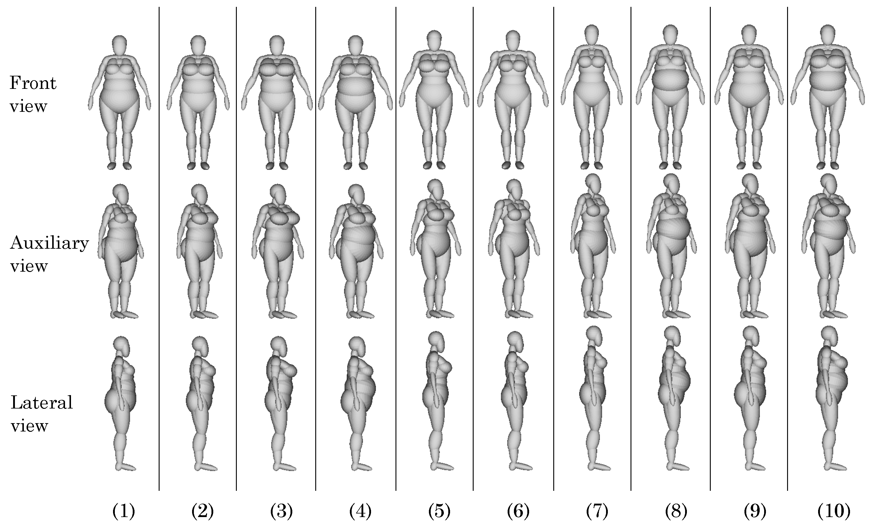
4.1. Measurement-Driven Models Generated via Interpolation

We synthesize a set of 243 measurement-driven mannequins from different sets of input measurements ($M{e}_f$). The sets of input measurements are generated by assigning three different values to each of the five tailor measurements that conform $M{e}_f$ and obtaining all possible combinations ($3^5=243$). These values correspond to the three intermediate quarters of the ranges of measurements defined by L.

The synthesis is performed via the segmented interpolation scheme presented in Section 3.6. Each synthesized mannequin is then measured with $m_T$ (see Section 3.5) in order to extract the resulting tailor measurements $x_t$ that produce its resulting geometry. Table 4 presents the relative error $ϵ=|\frac{x_t-M{e}_f}{M{e}_f}|\times 100$ between the resulting ($x_t$) and input ($M{e}_f$) measurements. This error is intended to display the accuracy with which the measurement-driven mannequins satisfy their input measurements. Figure 18 presents a sample of 10 randomly selected mannequins (see Table 5) from the 243 measurement-driven mannequins in order to visualize variations of synthesized models.

Table 4. Relative error between input and real measurements in set of synthesized mannequins. Measurements performed with $m_T$.

	Height ($\mathit{H}\mathit{e}$)	Shoulder Width ($\mathit{S}\mathit{h}$)	Breast Perimeter ($\mathit{B}\mathit{r}$)	Waist Perimeter ($\mathit{W}\mathit{a}$)	Hip Perimeter ($\mathit{H}\mathit{i}$)
Average Error (%)	0.2	2.6	2.4	0.8	0.9
Maximum Error (%)	0.4	6.6	7.0	1.5	2.2
Minimum Error (%)	0.0	0.1	0.0	0.0	0.1

Table 4. Relative error between input and real measurements in set of synthesized mannequins. Measurements performed with $m_T$.

	Height ($\mathit{H}\mathit{e}$)	Shoulder Width ($\mathit{S}\mathit{h}$)	Breast Perimeter ($\mathit{B}\mathit{r}$)	Waist Perimeter ($\mathit{W}\mathit{a}$)	Hip Perimeter ($\mathit{H}\mathit{i}$)
Average Error (%)	0.2	2.6	2.4	0.8	0.9
Maximum Error (%)	0.4	6.6	7.0	1.5	2.2
Minimum Error (%)	0.0	0.1	0.0	0.0	0.1

Table 5. Tailor measurements of mannequins shown in Figure 18 and Figure 19. Measurements in cm.

Mannequin	Height ($\mathit{H}\mathit{e}$)	Shoulder Width ($\mathit{S}\mathit{h}$)	Breast Perimeter ($\mathit{B}\mathit{r}$)	Waist Perimeter ($\mathit{W}\mathit{a}$)	Hip Perimeter ($\mathit{H}\mathit{i}$)
(1)	153.75	35.75	101.25	102.5	134.75
(2)	153.75	35.75	118.5	102.5	117.5
(3)	153.75	41.5	135.75	102.5	117.5
(4)	153.75	47.25	118.5	122.25	134.75
(5)	159.5	41.5	118.5	82.75	117.5
(6)	159.5	47.25	101.25	82.75	117.5
(7)	165.25	35.75	101.25	82.75	117.5
(8)	165.25	41.5	101.25	122.25	117.5
(9)	165.25	41.5	118.5	102.5	134.75
(10)	165.25	47.25	135.75	122.25	117.5

Table 5. Tailor measurements of mannequins shown in Figure 18 and Figure 19. Measurements in cm.

Mannequin	Height ($\mathit{H}\mathit{e}$)	Shoulder Width ($\mathit{S}\mathit{h}$)	Breast Perimeter ($\mathit{B}\mathit{r}$)	Waist Perimeter ($\mathit{W}\mathit{a}$)	Hip Perimeter ($\mathit{H}\mathit{i}$)
(1)	153.75	35.75	101.25	102.5	134.75
(2)	153.75	35.75	118.5	102.5	117.5
(3)	153.75	41.5	135.75	102.5	117.5
(4)	153.75	47.25	118.5	122.25	134.75
(5)	159.5	41.5	118.5	82.75	117.5
(6)	159.5	47.25	101.25	82.75	117.5
(7)	165.25	35.75	101.25	82.75	117.5
(8)	165.25	41.5	101.25	122.25	117.5
(9)	165.25	41.5	118.5	102.5	134.75
(10)	165.25	47.25	135.75	122.25	117.5

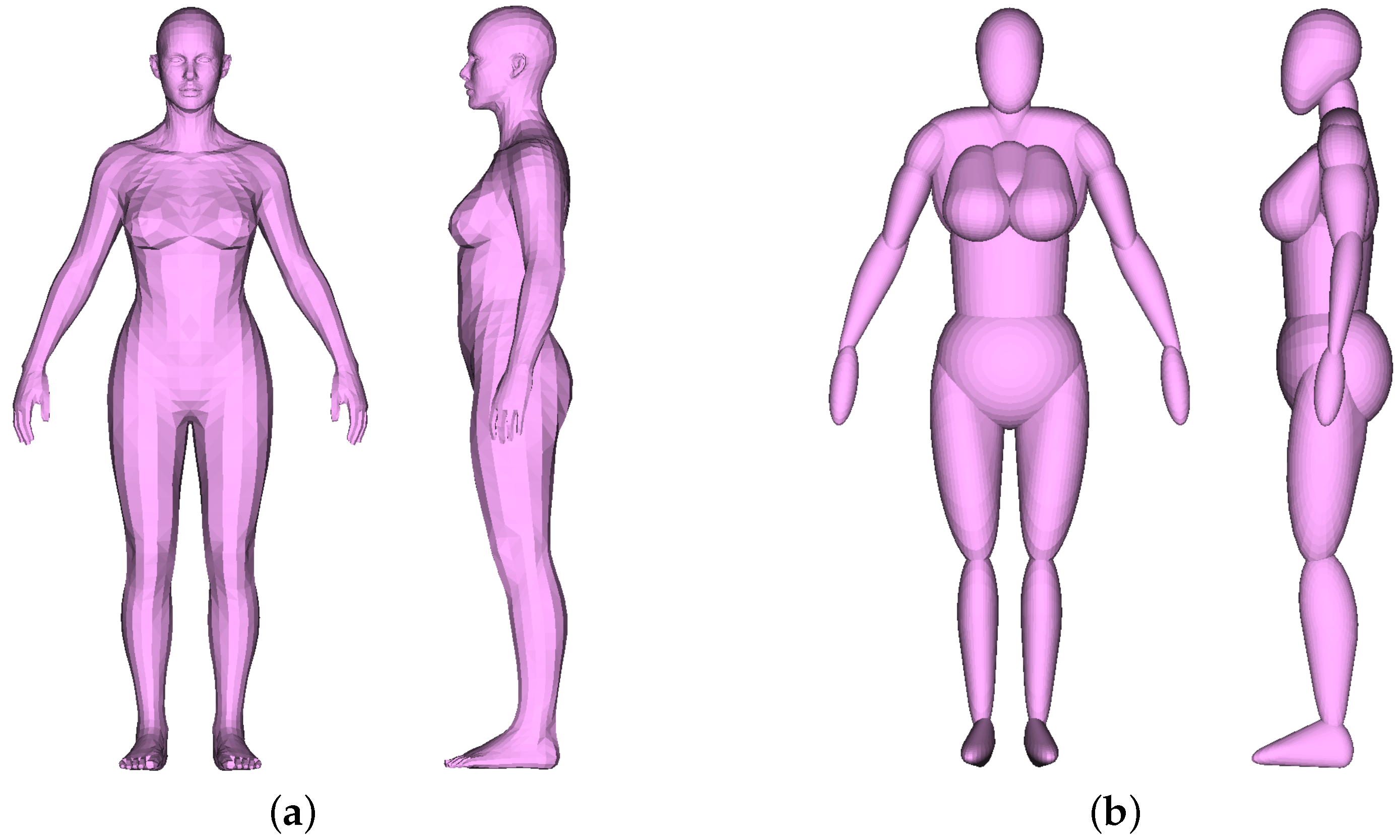
4.2. Quantitative Comparison: Cushion-Based Mannequin vs. Mesh-Based Model

We extracted the tailor measurements from a mesh-based primogenial model (see Table 2). These measurements served as the input and goal for the synthesis of an ellipsoid- or cushion-based mannequin. Tailor measurements were extracted from both and are compared in

Table 6. Relative error between Mesh-based Model and Cushion-based Mannequin measurements (cm). Measurements performed with $m_T$.

	Height (He)	Shoulder Width (Sh)	Breast Perimeter (Br)	Waist Perimeter (Wa)	Hip Perimeter (Hi)
Mesh-based Model	170	42.8	99.8	72.5	99.7
Cushion-based Mannequin	170.4	43.3	104.2	67.2	97.2
Error (%)	0.2	1.2	4.4	7.3	2.5

. A visual comparison can be seen in Figure 20.

4.3. Interaction Simulation between Convex Volume Model and Garment

We performed two soft-body (garment) vs. rigid-body (measurement-driven mannequin) interaction simulations using a physics engine (Ammo.js [5]). These simulations were executed in real-time and are intended to exhibit the usefulness of the convex-volume-based measurement-driven mannequins in garment-fitting simulation. The two simulations can be seen in Figure 21 and Figure 22, in which it is visible that the garments fit the shape of the mannequins.

Since the mannequins are already sets of convex volumes, no convex decomposition is required for collision detection, avoiding additional processing steps. Specific details of the configuration of the physics engine, the soft-body, and the rigid-body are not provided since they are not relevant to the focal point of this manuscript. This manuscript’s purpose is to present the modeling scheme for the measurement-driven mannequins, not to design garments nor to specify their interaction with the mannequins. Further research will focus on applications using the mannequins, such as garment-fitting simulation and its details.

5. Conclusions and Future Work

This manuscript presents a parametric modeling scheme for digital mannequins that represents the female human body as a set of convex volumes. Such a scheme allows synthesis of mannequins that satisfy the specified (input) tailor measurements with an average deviation of $1.5\%$, as presented in Table 4. The aforementioned hold a reasonable and realistic demeanor. The scheme also allows a wide variety of phenotypes across different ethnic groups to be approximated without any athletic idealization (see Figure 18).

The proposed modeling scheme contrasts with those found in the literature due to our mannequins being created with convex volumes as opposed to non-convex meshes (see Section 2). This results in our method holding the following advantages: (1) reduced computational costs and data storage; (2) reduced tuning for parameterization due to the small number of parameters used; (3) since the ellipsoids have attached coordinate systems (as robotic limbs), our formulation opens opportunities for straightforward motion modeling; and (4) no need for recomputing surface (skin) for pose definition. In addition, the mannequins are shown to be economical for garment-fitting simulation. This is due to the fact that the processing steps needed for preparing non-convex models for garment-fitting simulation (collision detection) [42,43,44,45,46,47,48] are avoided by already having a set of convex volumes.

Notice that our approach produces a gross approximation of pose and demeanor of the digital mannequin by using a set of convex primitives (whose boolean union is obviously non-convex). On the other hand, the existing literature uses detailed triangular meshes to express the mannequin. This difference in intention (coarse vs. detailed shapes) prevents a fair numerical comparison between our method and existing methods.

Future work is encouraged to define motion modeling (pose definition). Moreover, it is encouraged to extend the convex volume modeling scheme to model male human bodies and to expand the set of measurements (e.g., including crotch length) that define parameterization. It is important to keep in mind that this manuscript already achieves a wide variety of mannequins with a reduced number of parameters. Adding more measurement parameters will allow for the creation of more-intricate mannequins but will require more tuning.

Our convex (ellipsoid or cushion) volume approximation of a 3D female humanoid avoids explicit computation of the humanoid skin. When the humanoid changes pose, the convex components can be repositioned via their attached SO(3) coordinate frame. If needed, the skin of the humanoid may be computed via alpha-shape approaches for the current humanoid instead of modifying a hypothetical skin of the previous humanoid. Figure 23 displays a hint for skin computation (using Blender™) for our convexly decomposed humanoid. We point out that this initiative is not the aim of the present manuscript, rather for future ones.

References

1. Cheng, Z.Q.; Chen, Y.; Martin, R.R.; Wu, T.; Song, Z. Parametric modeling of 3D human body shape—A survey. Comput. Graph. 2018, 71, 88–100. [Google Scholar] [CrossRef]
2. Chu, C.H.; Tsai, Y.T.; Wang, C.C.; Kwok, T.H. Exemplar-based statistical model for semantic parametric design of human body. Comput. Ind. 2010, 61, 541–549. [Google Scholar] [CrossRef]
3. Liu, K.; Zeng, X.; Bruniaux, P.; Wang, J.; Kamalha, E.; Tao, X. Fit evaluation of virtual garment try-on by learning from digital pressure data. Knowl.-Based Syst. 2017, 133, 174–182. [Google Scholar] [CrossRef]
4. Wu, N.; Deng, Z.; Huang, Y.; Liu, C.; Zhang, D.; Jin, X. A fast garment fitting algorithm using skeleton-based error metric. Comput. Animat. Virtual Worlds 2018, 29, e1811. [Google Scholar] [CrossRef]
5. AMMO.JS—JavaScript Physics Engine. Port from Bullet. Available online: https://github.com/kripken/ammo.js/ (accessed on 10 December 2020).
6. Dang, L.M.; Min, K.; Wang, H.; Piran, M.J.; Lee, C.H.; Moon, H. Sensor-based and vision-based human activity recognition: A comprehensive survey. Pattern Recognit. 2020, 108, 107561. [Google Scholar] [CrossRef]
7. Lara, O.D.; Labrador, M.A. A survey on human activity recognition using wearable sensors. IEEE Commun. Surv. Tutor. 2012, 15, 1192–1209. [Google Scholar] [CrossRef]
8. Chen, Y.; Song, Z.; Xu, W.; Martin, R.R.; Cheng, Z.Q. Parametric 3D modeling of a symmetric human body. Comput. Graph. 2019, 81, 52–60. [Google Scholar] [CrossRef]
9. Chen, Y.; Liu, Z.; Zhang, Z. Tensor-based human body modeling. In Proceedings of the IEEE Conference on Computer Vision and Pattern Recognition, Portland, OR, USA, 23–28 June 2013; pp. 105–112. [Google Scholar]
10. Cho, Y.; Okada, N.; Park, H.; Takatera, M.; Inui, S.; Shimizu, Y. An interactive body model for individual pattern making. Int. J. Cloth. Sci. Technol. 2005, 17, 91–99. [Google Scholar] [CrossRef]
11. Cichocka, A.; Bruniaux, P.; Frydrych, I. 3D Garment Modelling-Creation of a Virtual Mannequin of the Human Body; Instytut Biopolimerów i Włókien Chemicznych (IBWCh): Łódź, Polska, 2014. [Google Scholar]
12. Huang, L.; Gao, C. Nonuniform Parametric Human Body Based on Model Reuse. In Proceedings of the 2014 5th International Conference on Digital Home, Guangzhou, China, 28–30 November 2014; pp. 406–411. [Google Scholar]
13. Kim, S.; Park, C.K. Parametric body model generation for garment drape simulation. Fibers Polym. 2004, 5, 12–18. [Google Scholar] [CrossRef]
14. Peng, J.; Jiang, G.; Cong, H. Rapid parametric human modeling in 3D garment simulation. Autex Res. J. 2019, 19, 60–67. [Google Scholar] [CrossRef] [Green Version]
15. Seo, H.; Magnenat-Thalmann, N. An automatic modeling of human bodies from sizing parameters. In Proceedings of the 2003 Symposium on Interactive 3D Graphics, Monterey, CA, USA, 27–30 April 2003; pp. 19–26. [Google Scholar]
16. Kasap, M.; Magnenat-Thalmann, N. Parameterized human body model for real-time applications. In Proceedings of the 2007 International Conference on Cyberworlds (CW’07), Hannover, Germany, 24–26 October 2007; pp. 160–167. [Google Scholar]
17. Baek, S.Y.; Lee, K. Parametric human body shape modeling framework for human-centered product design. Comput.-Aided Des. 2012, 44, 56–67. [Google Scholar] [CrossRef]
18. Baek, S.Y.; Lee, K. Parametric human body modelling system for virtual garment fitting. Int. J. Comput. Aided Eng. Technol. 8 2013, 5, 242–261. [Google Scholar] [CrossRef]
19. Goncharenko, I.; Takashiba, K.; Mochimaru, M.; Kouchi, M.; Usui, S.; Odahara, M. Low-parametric control of human body shape modelling via the web using 3D scan data. Int. J. Hum. Factors Model. Simul. 1 2012, 3, 187–203. [Google Scholar] [CrossRef]
20. Hasler, N.; Stoll, C.; Sunkel, M.; Rosenhahn, B.; Seidel, H.P. A statistical model of human pose and body shape. In Computer Graphics Forum; Blackwell Publishing Ltd.: Oxford, UK, 2009; Volume 28, pp. 337–346. [Google Scholar]
21. Koo, B.Y.; Park, E.J.; Choi, D.K.; Kim, J.J.; Choi, M.H. Example-based statistical framework for parametric modeling of human body shapes. Comput. Ind. 2015, 73, 23–38. [Google Scholar] [CrossRef]
22. Wang, C.C. Parameterization and parametric design of mannequins. Comput.-Aided Des. 2005, 37, 83–98. [Google Scholar] [CrossRef]
23. Huang, J.; Kwok, T.H.; Zhou, C. Parametric design for human body modeling by wireframe-assisted deep learning. Comput.-Aided Des. 2019, 108, 19–29. [Google Scholar] [CrossRef]
24. Loper, M.; Mahmood, N.; Romero, J.; Pons-Moll, G.; Black, M.J. SMPL: A skinned multi-person linear model. ACM Trans. Graph. (TOG) 2015, 34, 1–16. [Google Scholar] [CrossRef]
25. Pujades, S.; Mohler, B.; Thaler, A.; Tesch, J.; Mahmood, N.; Hesse, N.; Bülthoff, H.H.; Black, M.J. The virtual caliper: Rapid creation of metrically accurate avatars from 3D measurements. IEEE Trans. Vis. Comput. Graph. 2019, 25, 1887–1897. [Google Scholar] [CrossRef]
26. Hilton, A.; Beresford, D.; Gentils, T.; Smith, R.; Sun, W.; Illingworth, J. Whole-body modelling of people from multiview images to populate virtual worlds. Vis. Comput. 2000, 16, 411–436. [Google Scholar] [CrossRef]
27. Lee, W.; Gu, J.; Magnenat-Thalmann, N. Generating animatable 3D virtual humans from photographs. In Computer Graphics Forum; Blackwell Publishers Ltd.: Oxford, UK; Boston, MA, USA, 2000; Volume 19, pp. 1–10. [Google Scholar]
28. Wang, C.C.; Wang, Y.; Chang, T.K.; Yuen, M.M. Virtual human modeling from photographs for garment industry. Comput.-Aided Des. 2003, 35, 577–589. [Google Scholar] [CrossRef]
29. Xu, Z.; Chang, W.; Zhu, Y.; Dong, L.; Zhou, H.; Zhang, Q. Building high-fidelity human body models from user-generated data. IEEE Trans. Multimed. 2020, 23, 1542–1556. [Google Scholar] [CrossRef]
30. Gu, L.; Istook, C.; Ruan, Y.; Gert, G.; Liu, X. Customized 3D digital human model rebuilding by orthographic images-based modelling method through open-source software. J. Text. Inst. 2019, 110, 740–755. [Google Scholar] [CrossRef]
31. Kolotouros, N.; Pavlakos, G.; Daniilidis, K. Convolutional mesh regression for single-image human shape reconstruction. In Proceedings of the IEEE/CVF Conference on Computer Vision and Pattern Recognition, Long Beach, CA, USA, 15–20 June 2019; pp. 4501–4510. [Google Scholar]
32. Xie, H.; Zhong, Y.; Yu, Z.; Hussain, A. Non-parametric anthropometric graph convolutional network for virtual mannequin reconstruction. IEEE Access 2019, 8, 3539–3550. [Google Scholar] [CrossRef]
33. Scheepers, F.; Parent, R.E.; Carlson, W.E.; May, S.F. Anatomy-based modeling of the human musculature. In Proceedings of the 24th Annual Conference on Computer Graphics and Interactive Techniques, Los Angeles, CA, USA, 3–8 August 1997; pp. 163–172. [Google Scholar]
34. Wilhelms, J.; Van Gelder, A. Anatomically based modeling. In Proceedings of the 24th Annual Conference on Computer Graphics and Interactive Techniques, Los Angeles, CA, USA, 3–8 August 1997; pp. 173–180. [Google Scholar]
35. Qin, K.; Zhuang, Y.; Wu, F. Parameterizing 3D Human Model in Garment CAD. J. Comput. Aided Des. Comput. Graph. 2004, 16, 5. [Google Scholar]
36. Seo, H.; Magnenat-Thalmann, N. An example-based approach to human body manipulation. Graph. Model. 2004, 66, 1–23. [Google Scholar] [CrossRef]
37. Edelsbrunner, H.; Mücke, E.P. Three-dimensional alpha shapes. ACM Trans. Graph. (TOG) 1994, 13, 43–72. [Google Scholar] [CrossRef]
38. Ouahabi, A. Signal and Image Multiresolution Analysis; John Wiley & Sons: Hoboken, NJ, USA, 2012. [Google Scholar]
39. Kaneflame3d. Realistic White Male and Female Low Poly: 3D Model. Available online: https://www.cgtrader.com/free-3d-models/character/anatomy/realistic-white-male-and-female-low-poly (accessed on 12 August 2021).
40. Coyte, J.L.; Stirling, D.; Du, H.; Ros, M. Seated whole-body vibration analysis, technologies, and modeling: A survey. IEEE Trans. Syst. Man Cybern. Syst. 2015, 46, 725–739. [Google Scholar] [CrossRef]
41. THREE.JS—JavaScript 3D Library. Available online: https://threejs.org/ (accessed on 10 December 2020).
42. Backenhof, A. Automatic Generation of Collision Hulls for Polygonal Objects; Linkoping University Electronic Press: Linkoping, Sweden, 2011. [Google Scholar]
43. Bäcklund, H.; Neijman, N. Automatic Mesh Decomposition for Real-Time Collision Detection; Linköping University: Linköping, Sweden, 2014. [Google Scholar]
44. Chowriappa, A.; Wirz, R.; Ashammagari, A.R.; Kesavadas, T. A convex decomposition methodology for collision detection. In Proceedings of the 2013 IEEE Virtual Reality (VR), Lake Buena Vista, FL, USA, 18–20 March 2013; pp. 57–58. [Google Scholar]
45. Ghosh, M.; Amato, N.M.; Lu, Y.; Lien, J.M. Fast approximate convex decomposition using relative concavity. Comput.-Aided Des. 2013, 45, 494–504. [Google Scholar] [CrossRef]
46. Liu, H.; Liu, W.; Latecki, L.J. Convex shape decomposition. In Proceedings of the 2010 IEEE Computer Society Conference on Computer Vision and Pattern Recognition, San Francisco, CA, USA, 13–18 June 2010; pp. 97–104. [Google Scholar]
47. Mamou, K.; Ghorbel, F. A simple and efficient approach for 3D mesh approximate convex decomposition. In Proceedings of the 2009 16th IEEE international conference on image processing (ICIP), Cairo, Egypt, 7–10 November 2009; pp. 3501–3504. [Google Scholar]
48. Müller, M.; Heidelberger, B.; Hennix, M.; Ratcliff, J. Position based dynamics. J. Vis. Commun. Image Represent. 2007, 18, 109–118. [Google Scholar] [CrossRef] [Green Version]
Figure 1. Flow diagram of the convex-volume-based measurement-driven approximation. Input: Reference 3D model. Output: Measurement-driven mannequin B. Steps 1 and 2 pre-processing. Steps 3 and 4 are processing.
Applsci 12 09742 g001
Figure 2. Reference 3D model to be approximated by convex volumes. Planar data (red lines).
Applsci 12 09742 g002
Figure 3. Approximation of the left thigh and hip with ellipsoids, front and lateral views. Red dotted line: surface boundary to approximate. (a) Approximation with one ellipsoid. (b) Improvement of the approximation with a second ellipsoid.
Applsci 12 09742 g003
Figure 4. Approximation of the reference 3D model with ellipsoids with resulting Base Mannequin ( B M ) and ellipsoid mannequin and no cushions computed. (a) Half of the body approximated. (b) The full body approximated and mirroring executed.
Applsci 12 09742 g004
Figure 5. Map used to convert ellipsoids into cushions, topology map and ellipsoid model. Pairs of ellipsoids with same color form a cushion.
Applsci 12 09742 g005
Figure 6. Example of cushion C E 1 E 2 , arbitrarily oriented and positioned ellipsoids ( E 1 and E 2 ) in space with convex hull operation between E 1 and E 2 . (a) Ellipsoids E 1 and E 2 . (b) Cushion C E 1 E 2 between ellipsoids E 1 and E 2 .
Applsci 12 09742 g006
Figure 7. Mannequin approximated with cushions and ellipsoids. Ellipsoid mannequin (a) for comparison. Cushions computed according to Figure 5. Small chubby mannequin (see Section 3.3) as (a) Ellipsoid-based Mannequin and (b) Cushion-based Mannequin.
Applsci 12 09742 g007
Figure 8. Flow diagram for the construction of R M based on B M . Process for a single R M i R M .
Applsci 12 09742 g008
Figure 9. Set R M of Reference Mannequins as ellipsoid mannequins (no cushions) of extreme and average models. From left to right: Small Chubby, Small Slim, Average, Tall Slim, and Tall Chubby.
Applsci 12 09742 g009
Figure 10. Anatomical planes defined for the Reference Mannequins.
Applsci 12 09742 g010
Figure 11. World Coordinate System definition, registration process, and definition of pivot point (origin) of WCS. (a) Orthogonal views. (b) Isometric view.
Applsci 12 09742 g011
Figure 12. Minimization of the variation between orientations of corresponding ellipsoids with re-labeling and direction inversion. Yellow ellipsoids, 13.a Rectus Abdominalis from Tall Chubby (reference [ u c , v c , w c ] ) and Tall Slim (modified orientation [ u , v , w ] ). (a) Incorrect status for axes u , v , w . (b) Re-labeled axes u , v , w in (a). Correct labeling, incorrect direction for axes u , v , w . (c) Direction inversion of axes u , v , w in (b). Correct status for axes u , v , w .
Applsci 12 09742 g012
Figure 13. Correction of lateral ellipsoid symmetry of ellipsoids from Tall Chubby with only legs displayed for the example. (a) Asymmetric model. (b) Symmetric model.
Applsci 12 09742 g013
Figure 14. Correction of central ellipsoid symmetry of ellipsoids from Tall Chubby. (a) Asymmetric model. (b) Symmetric model.
Applsci 12 09742 g014
Figure 15. Tailor measuring of ellipsoid mannequins with heights at which m T ( ) is applied and example of cross sections obtained and measured with m T ( ) of breast and hips of Small Slim ellipsoid model. (a) Heights at which 2D convex hulls are computed. (b) Examples of 2D convex hulls.
Applsci 12 09742 g015
Figure 16. Body subsets of ellipsoids for segmented interpolation scheme. Each subset is interpolated with different subsets of the input measurements M e . (a) Measurement dependency for body neighborhoods (subsets of ellipsoids). (b) Example of subsets of ellipsoids influenced by different measurements.
Applsci 12 09742 g016
Figure 17. Example of synthesized lower body neighborhoods using segmented interpolation scheme. Synthesized mannequins are transparent. Reference Mannequins (RM) are marked with R M i . R M 1 : Small Chubby. R M 2 : Tall Chubby. R M 3 : Small Slim. R M 4 : Tall Slim.
Applsci 12 09742 g017
Figure 18. Examples of synthesized ellipsoid-based mannequins using segmented interpolation approach.
Applsci 12 09742 g018
Figure 19. Cushion-based mannequins. These mannequins correspond to the same mannequins in Figure 18 with ellipsoids converted to cushions.
Applsci 12 09742 g019
Figure 20. Visual comparison of Mesh-based Model vs. Cushion-based Mannequin synthesized using the measurements from the Mesh-based Model. (a) Mesh-based Model. (b) Cushion-based Mannequin.
Applsci 12 09742 g020
Figure 21. Interaction simulation of Slim Tall model and garment using cushion model and showing rigid-body vs. soft-body interaction. Visualization: Constructed by us in Three.js [41]. Simulation: Constructed by us in Ammo.js [5]. (a) Solid-color garment. (b) Wireframe garment.
Applsci 12 09742 g021
Figure 22. Interaction simulation of Chubby Small model and scaled garment using cushion model and showing rigid-body vs. soft-body interaction. Visualization: Constructed by us in Three.js [41]. Simulation: Constructed by us in Ammo.js [5]. (a) Scaled garment. (b) Wireframe scaled garment.
Applsci 12 09742 g022
Figure 23. Smooth representations of the Cushion-based Mannequins. These representations are not the aim of the present manuscript, rather for future ones.
Applsci 12 09742 g023