Study on Reinforcement Mechanism and Reinforcement Effect of Saturated Soil with a Weak Layer by DC

Abstract

This paper presents a numerical investigation on the improvement mechanism of dynamic compaction (DC) in saturated soil of a weak layer with high levels of groundwater, using an improved fluid–solid coupling method with a Drucker–Prager–Cap soil model. The numerical model is verified by comparing with published test data at first, which show that the dual-phase coupling method can approximately reflect the development law of excess pore water pressure and the improvement effect of layered saturated soil foundation under DC. Then, based on the numerical model, the influences of the thickness and depth of the weak layer as well as tamping energy on the development and dissipation of excess pore water pressure, effective stress, and the relative degree of reinforcement during DC were investigated. The results showed that the embedment depth and thickness of the weak interlayer may greatly affect the effective reinforcement depth of DC. Meanwhile, the tamping energy and the groundwater table also play a great role in the improvement of the layered saturated soil under DC. The groundwater table should be lowered by dewatering or adding a drainage layer to achieve a better compaction effect during DC.

1. Introduction

1.1. Background

Grounds with unsuitable conditions, such as liquefiable soils and a weak foundation, directly influence the safety of construction, and at the same time it will also affect the work quality and construction schedule in civil engineering construction, and in appropriate disposal of a foundation, treatment can cause severe problems of construction quality. In order to improve the bearing capacity of soft foundation, enhance its resistance to vibration liquefaction, eliminate post-construction differential settlement, and save project costs, these poor engineering geological sites should be treated [1,2,3,4,5].

1.2. Dynamic Compaction

Dynamic compaction (DC) is a fast, simple, and widely used foundation treatment method, which can improve the bearing capacity [6,7] and reduce the liquefaction-inducted damage [8,9] of various foundations. Compared to many other ground improvement techniques, DC has the advantages in improvement depth, cost-effectiveness, convenience, and adaptability to a broad range of soils [10,11,12,13].

Table 1. Summary of previous research on DC through field tests, numerical simulation, and experimental models [14,15,16,17,18,19,20,21,22,23].

Reference	Ground Stratum	Research Questions	Main Conclusion	Investigation Method
Lee, F. H., & Gu, Q. [14]	Uniform	A two-dimensional finite element method based on the cap model is used to study the influence of different construction parameters and soil properties on the reinforcement effect by DC.	This paper proposes a chart method for predicting the reinforcement effect of sandy soil foundation.	Numerical method
Wang et al. [15]	Uniform	Ls-dyna was used to investigate influence of different parameters of DC and soil properties’ conditions.	This paper presents a estimation method for ground deformation of granular soils caused by DC.	Numerical method
Dou et al. [16]	Uniform	A three-dimensional finite element analysis is conducted to investigate the influence of soil properties, different parameters of DC on the soil improvement between adjacent tamping locations by multi-point tamping.	This paper proposes a method for estimating the degree of final soil improvement between adjacent tamping locations.	Numerical method
Zhou et al. [17]	Uniform	This paper developed a the fluid–solid coupled method incorporating the cap model to analyze the improvement on saturated foundation by DC.	This paper focuses on the two key elements, which influenced improvement of saturated foundation: groundwatertable and sitecondition.	Numerical method
Zhou et al. [18]	Uniform	A three-dimensional (3D) finite element (FE) model based on cap modelis established to deal with the problem of the factors affecting the sandy soil improvement effect.	A formula considering the various factors of DC is put forward to predict the reinforcement effect by DC	Numerical method
Perucho, A., & Olalla, C. [19]	a plastic clayey fill in a port area	Dynamic consolidation was used to reinforce a plastic clay in the infill port area.	Dynamic consolidation proved to be an effective form of soft foundation treatment for plastic clayey fill in a port area.	Field test
Feng et al. [20]	soft soils	The dynamic consolidation (heavy tamping) is performed in a site with loosely deposited soft soils in the Yangtze River Delta of China.	The allowable bearing capacity and the depth of improvement after DC meet the design requirements.	Field test
Feng et al. [21]	Uniform	A novel method of modeling preloading consolidation and DC in centrifuge are developed in this study.	The results of test are comprehensively analyzed and discussed to have a better understanding of preloading consolidation and DC.	Centrifuge test
Jia et al. [22]	Uniform	Model tests of DC on sand with different groundwater tables are performed to investigate the effect of groundwater depth in DC.	Through the comparison of dynamic responses of soils, dewatering is used for the treatment of saturated soil with groundwater.	Model tests
Abdizadeh et al. [23]	Uniform	ABACUS 6.14 software is used to simulate three-dimensional model of lateral DC in the slope.	Impact velocity is the major factor that influences soil improvement for three different slope.	Numerical method

[14,15,16,17,18,19,20,21,22,23] summarizes the studies in which the improvement mechanism and effects of DC through field tests, numerical simulation, and experimental models have been investigated. In many of these studies, the ground stratum was idealized as uniform for simplicity. However, in reality, the ground conditions are often much more complex, which may include layered soils with varying groundwater level. The changes of ground conditions may greatly influence the compaction efficiency (e.g., fall down of the tamper due to local temporary liquefaction) and improvement effects of DC. Moreover, two factors must be considered in the design parameters and construction methods of DC, such as the soil type and groundwater level.

In the alluvial plain of the lower Yellow River, China, the ground is typically layered (e.g., layers of silty clay, silt, silty sand, and soft clay sometimes) along with long-term alluviation and sedimentation, and the strength, deformation, and permeability properties may vary significantly in layers. Meanwhile, the groundwater level is normally high. DC is one of the most commonly used ground improvement methods in this area [24,25]. Some pioneering studies [26,27,28] have attempted to investigate the performance of DC in this typical layered silty ground, and they have shown that the existence of soft soil interlayer obviously hinders the reinforcement effect and restrains further development of the effective reinforcement depth. However, the influences of the position and the thickness of weak interlayers on the compaction mechanism and improvement effects have rarely been studied. Furthermore, unlike the uniform saturated soil improvement, the pore pressure of the soil with a weak interlayer dissipates slowly, and there is a cushioning effect, which has a damping action on the transfer of impact energy.

1.3. Main Research Contents

This paper presents an improved fluid–solid coupling method with a Drucker–Prager–Cap model for saturated soil to investigate the improvement mechanism of DC for layered grounds with a weak interlayer. The numerical model based on finite element method (FEM) is introduced briefly at first and then validated by comparing with published test data. Using the FEM model, influences of the thickness and location of the soft interlayer under DC and tamping energy on the development of excess pore water pressure and improvement effects are studied. Finally, some engineering solutions are suggested to effectively improve the soil foundation with an embedded weak layer.

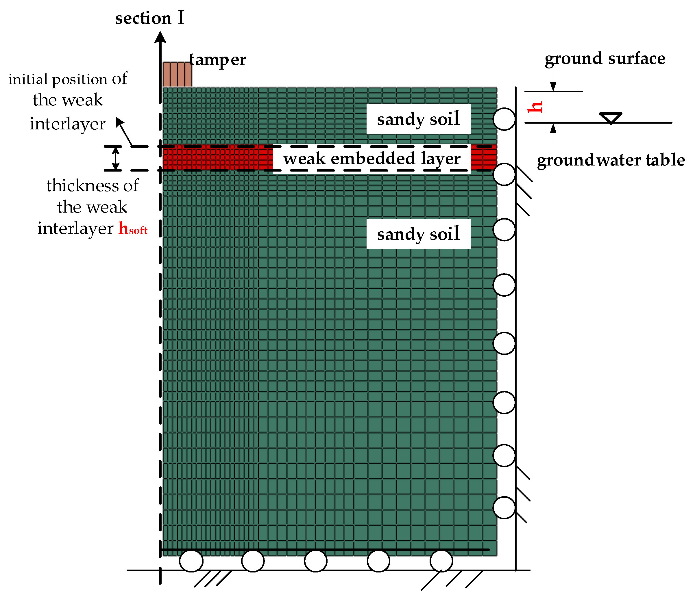
2. The Fluid–Solid Coupling Model and FEM Implementation

2.1. u-U-p Formulation

Based on the ABAQUS/explicit platform of Ye et al. [29,30], Zhou et al. [17,31] developed a fluid–solid coupling method with a Drucker–Prager–Cap model for the FEM analysis of DC. The u-U-p formulation is briefly introduced as follows.

The u-U-p formulation is given by:

$${\mathrm{L}}^{\mathrm{T}}\mathsf{\sigma }\text{'}+\left(\mathsf{\alpha }-\mathrm{n}\right)\nabla \mathrm{p}+\mathrm{c}\left(\dot{\mathrm{U}}-\dot{\mathrm{u}}\right)-\left(1-\mathrm{n}\right){\mathsf{\rho }}_{\mathrm{s}}\ddot{\mathrm{u}}+\left(1-\mathrm{n}\right){\mathsf{\rho }}_{\mathrm{s}}{\mathrm{b}}_{\mathrm{s}}=0$$

(1)

$$\mathrm{n}\nabla \mathrm{p}-\mathrm{c}\left(\dot{\mathrm{U}}-\dot{\mathrm{u}}\right)-\mathrm{n}{\mathsf{\rho }}_{\mathrm{f}}\ddot{\mathrm{U}}+\mathrm{n}{\mathsf{\rho }}_{\mathrm{f}}{\mathrm{b}}_{\mathrm{f}}=0$$

(2)

where u is solid displacement; U is pore fluid displacement; p is pore pressure; ρ_s and ρ_f are the densities of the soil grains and pore fluid, respectively; b_s and b_f are the body force vectors on the soil grains and pore fluid, respectively.

$$\mathrm{p}={\mathrm{K}}_{\mathrm{f}}\frac{\left(1-\mathrm{n}-\frac{\mathrm{K}\text{'}}{{\mathrm{K}}_{\mathrm{s}}}\right){\mathrm{m}}^{\mathrm{T}}\mathsf{\epsilon }+\mathrm{n}{\nabla }^{\mathrm{T}}\mathrm{U}}{\mathrm{n}+\left(1-\mathrm{n}\right)\frac{{\mathrm{K}}_{\mathrm{f}}}{{\mathrm{K}}_{\mathrm{s}}}-\frac{\mathrm{K}\text{'}{\mathrm{K}}_{\mathrm{f}}}{{\mathrm{K}}_{\mathrm{s}}^2}}$$

(3)

where m^T = [1 1 1 0 0 0] and ε is the strain vector of the soil skeleton (or solid domain), respectively; m^Tε = ε_v = volumetric strain; K’, K_f, and K_s are the bulk moduli of the soil skeleton, pore fluid, and soil grain, respectively; n = porosity.

$$\mathsf{\alpha }=1-\frac{\mathrm{K}\text{'}}{{\mathrm{K}}_{\mathrm{s}}}$$

(4)

$$\mathrm{c}=\frac{{\mathsf{\gamma }}_{\mathrm{f}}{\mathrm{n}}^2}{\mathrm{k}}$$

(5)

where γ_f and k are the unit weight and coefficient of permeability of the pore fluid, respectively.

$${\mathrm{L}}^{\mathrm{T}}=\left[\begin{array}{cccccc}\frac{\partial }{\partial \mathrm{x}}& 0& 0& \frac{\partial }{\partial \mathrm{y}}& 0& \frac{\partial }{\partial \mathrm{z}}\\ 0& \frac{\partial }{\partial \mathrm{y}}& 0& \frac{\partial }{\partial \mathrm{x}}& \frac{\partial }{\partial \mathrm{z}}& 0\\ 0& 0& \frac{\partial }{\partial \mathrm{z}}& 0& \frac{\partial }{\partial \mathrm{y}}& \frac{\partial }{\partial \mathrm{x}}\end{array}\right]$$

(6)

Both Equations (1) and (2) respectively comprise three separate equations, which relate to solid and fluid dynamic equilibrium in the x, y, and z directions. For the fluid–solid coupling soil assembles, pore fluid is supposed to be incompressible during DC.

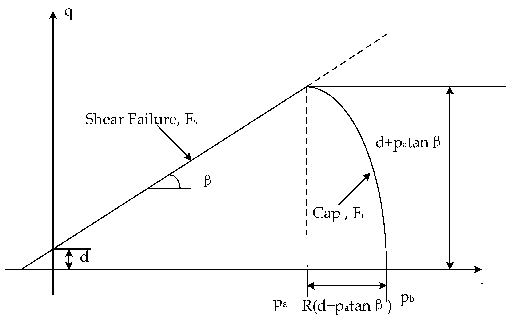
2.2. Constitutive Model for Soil in DC

The constitutive soil model used by Zhou et al. [17,31] is a cap plasticity hardening model with a non-hardening Drucker–Prager shearing surface, and it has been widely adopted for modeling the soil improvement effect of the foundation under DC [14,17,18,31,32]. As Figure 1 shows, a failure surface is applied herein put forward by Helwany [33].

$${\mathrm{F}}_{\mathrm{s}}=\mathrm{q}-\mathrm{p}\mathrm{t}\mathrm{a}\mathrm{n}\mathsf{\beta }-\mathrm{d}=0$$

(7)

An elliptical hardening cap surface is given by:

$${\mathrm{F}}_{\mathrm{c}}=\sqrt{{\left(\mathrm{p}-{\mathrm{p}}_{\mathrm{a}}\right)}^2+{\left(\mathrm{R}\mathrm{q}\right)}^2}-\mathrm{R}\left(\mathrm{d}+{\mathrm{p}}_{\mathrm{a}}\mathrm{t}\mathrm{a}\mathrm{n}\mathsf{\beta }\right)=0$$

(8)

where p and q are the mean stress and deviatoric stress, respectively; R is the curvature of the shape of the hardening cap, β is the soil’s angle of friction, and d is its cohesion in the p–q plane, as shown in Figure 1. The hardening parameter p_a is related to the hardening–softening behavior, which is defined as

$${\mathrm{p}}_{\mathrm{a}}=\frac{{\mathrm{p}}_{\mathrm{b}}-\mathrm{R}\mathrm{d}}{\left(1+{\mathrm{R}}^{\prime }\mathrm{t}\mathrm{a}\mathrm{n}\mathsf{\beta }\right)}$$

(9)

where p_b is the intersection of the cap surface with the p axis and is connected with the plastic volumetric change ${\mathsf{\epsilon }}_{\mathrm{v}}^{\mathrm{p}}$ by

$${\mathrm{p}}_{\mathrm{b}}=\frac{1}{3}\left[-\frac{1}{\mathrm{D}}\mathrm{l}\mathrm{n}\left(1-\frac{{\mathsf{\epsilon }}_{\mathrm{v}}^{\mathrm{p}}}{\mathrm{W}}\right)\right]+{\mathrm{p}}_0$$

(10)

where D and W are the material parameters, and p₀ is the in situ of mean ground stress.

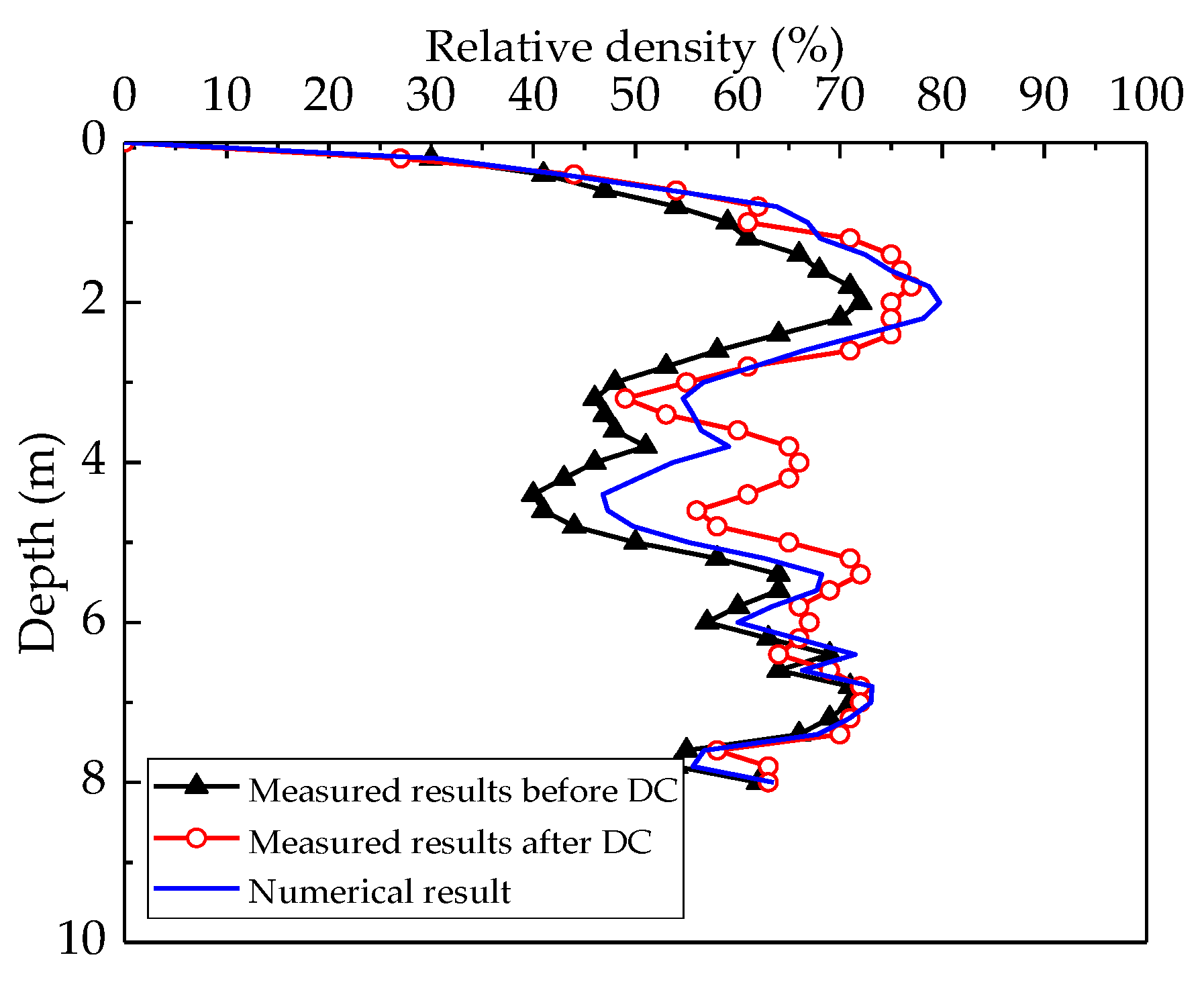
3. Validation of the Numerical Method

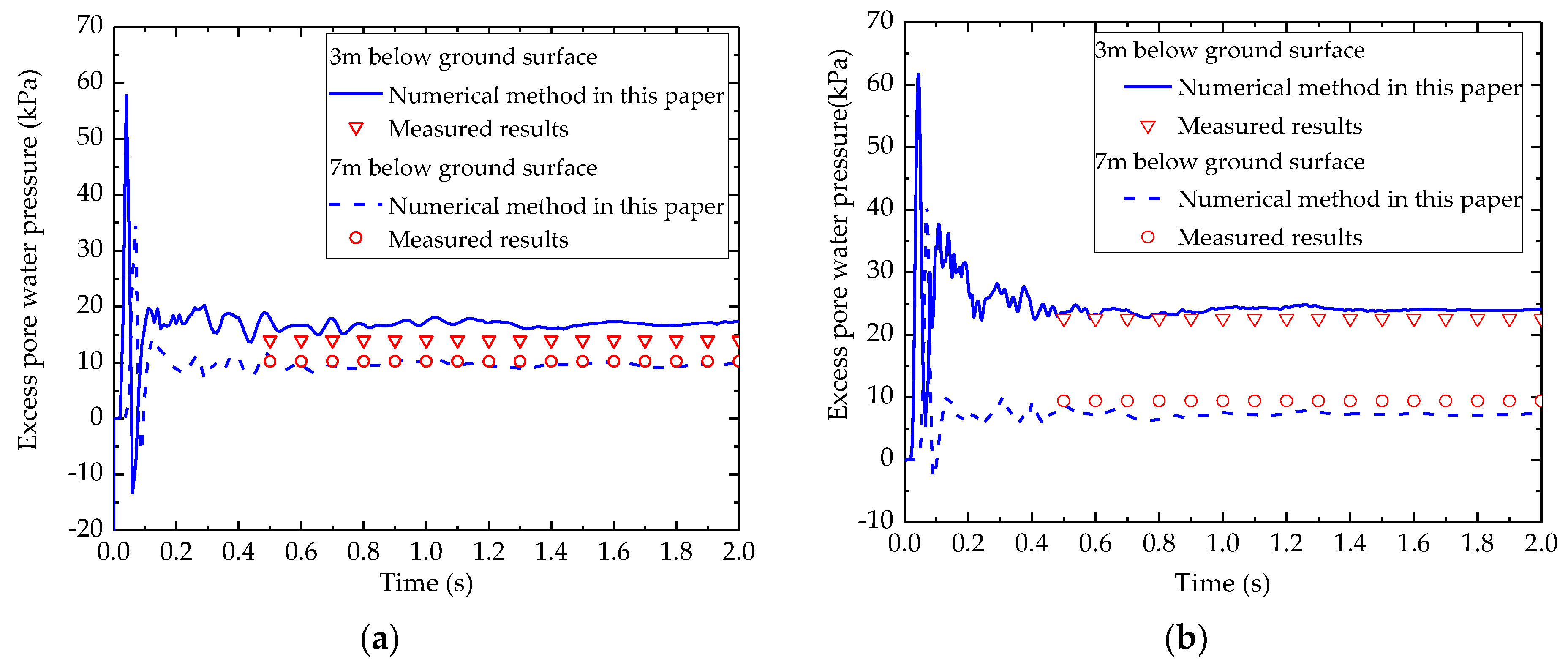
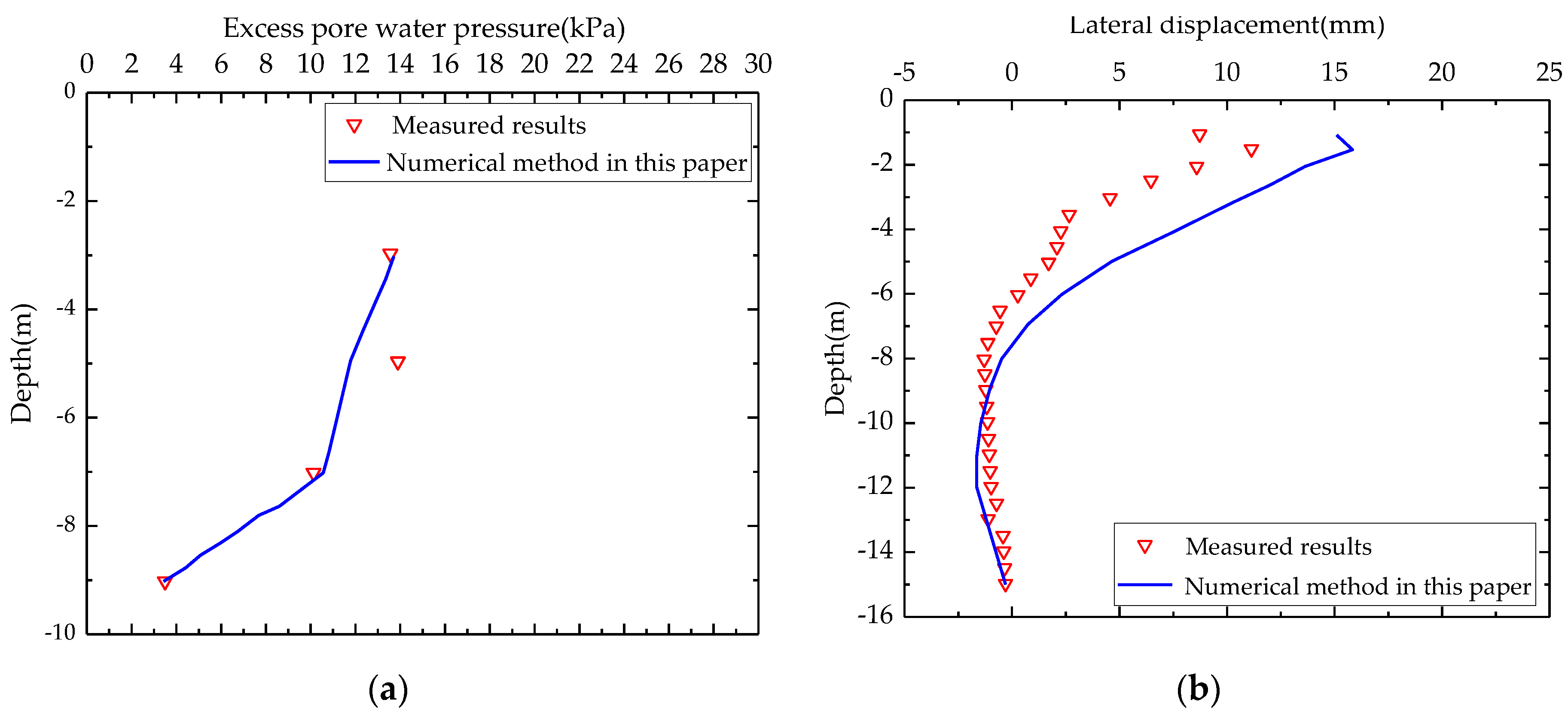
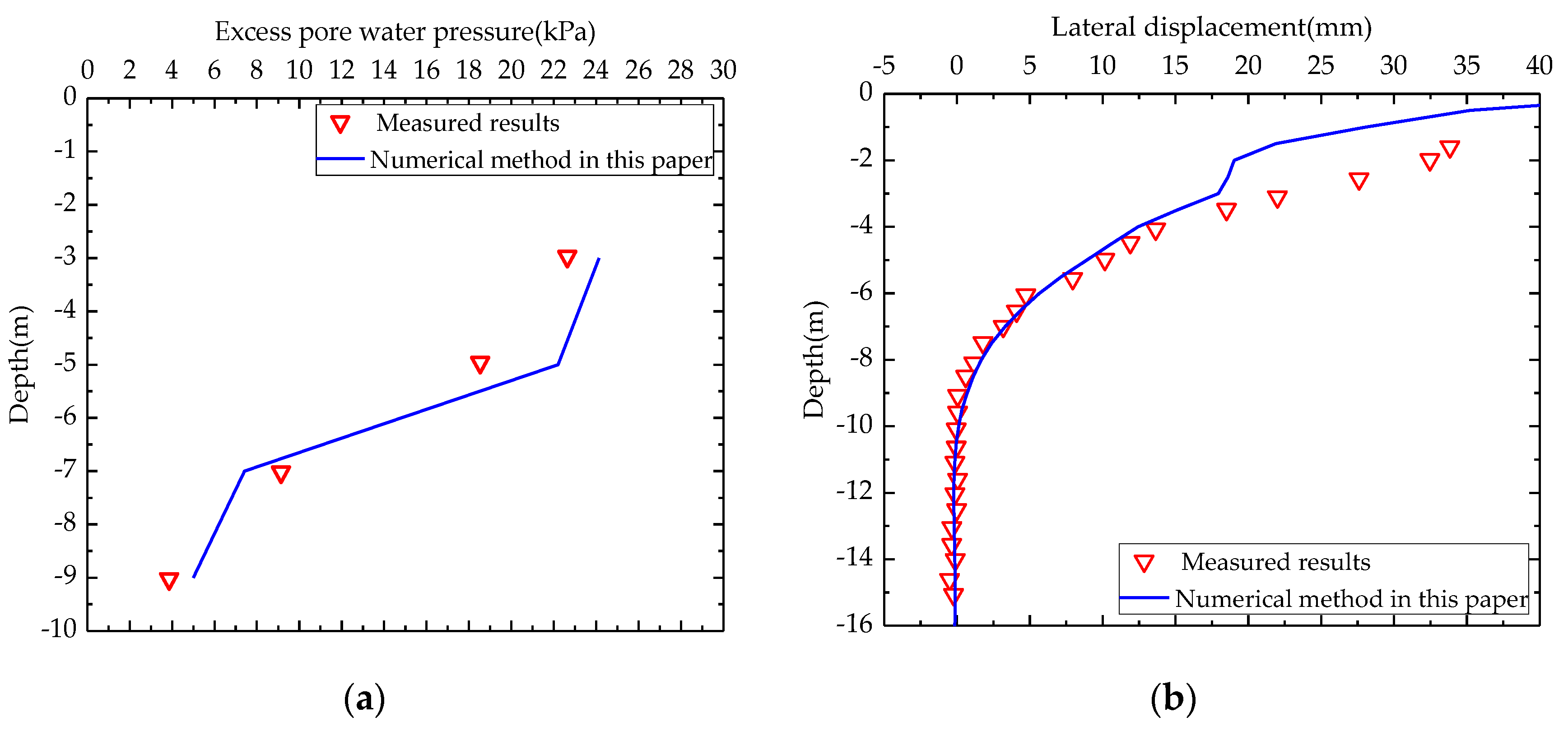
3.1. Pore Water Pressure and Lateral Displacement

The proposed Abaqus Dual-Phase Coupling Method with the cap hardening soil model was validated by Zhou et al. [17,31] using some field measurement data (pore pressure and soil displacement) [34]. It is not repeated here for brevity, but interested readers can refer to Zhou et al. [17,31]. The section mainly presents important data. Figure 2 shows the numerical computation of excess pore water pressure at 3 m and 7 m below ground surface during the first DC blow. The comparison results of lateral movement and excess pore water pressure at different depths for 1500 kN·m and 2500 kN·m were measured after the first blow, as presented in Figure 3 and Figure 4. Although there are some differences between numerical model and measuring result are observed, the changing laws of the numerical result coincide basically with those of measurements. In general, it is pretty reliable to use the Dual-Phase Coupling Method to predict the responses of saturated soils (stress, displacement, and pore pressure) during DC.

3.2. Reinforcement Effect

The reinforcement effect is not mentioned in the aforementioned verification. Therefore, the reliability of this method is further examined by comparing with field monitoring data of layered ground by DC reported by Chen et al. [26]. The foundation stratums, from the top down, were sandy soil, embedded weak silt clay layer, and sandy soil, as shown in Figure 5. In this study, the cap parameters of sandy soil used are the same as those of Zhou et al. [18,32]. The relevant parameter of the in-between weak layer was used and selected from those of Zhou et al. [17,31]. The coefficient of permeability of sandy soil and embedded weak layer soil and the bulk modulus of pore water are assumed to be 1 × 10⁻² m/s, 1 × 10⁻⁷ m/s, and 1 × 10⁴ kPa, respectively, based on Zhou et al.’s numerical analysis [17,31]. To sum up, the soil parameters used in the numerical simulation are shown in

Table 2. Soil parameters for DC analysis.

Soil Layer	ρ (kg/m3)	E (Mpa)	v	φ	c (kPa)	R	W	D (kPa−1)
Sand	1500	25.0	0.30	30°	10	4.33	0.4	0.00018
Weak layer	1500	10.0	0.30	0°	10	4.33	0.5	0.0003
Sand	1500	25.0	0.30	30°	10	4.33	0.4	0.00018

and

Table 3. Pore fluid parameters for DC analysis.

Soil Layer	ρf (kg/m3)	k (m/s)	v	Ks (kPa)	Kf (kPa)	n
Sand	1000	10−2	0.30	1 × 104	2.0 × 1011	0.4382
Weak layer	1000	10−7	0.30	1 × 104	2.0 × 1011	0.4382
Sand	1000	10−2	0.30	1 × 104	2.0 × 1011	0.4382

.

The FEM model contained 2000 solid meshes and 2000 fluid meshes, respectively. The whole model was 20 m in width and 30 m in height and divided into three layers. The FEM analysis was performed using a four-node axisymmetric quadrilateral element with reduced integration. The groundwater level was set on ground surface as reported [26]. The vertical boundaries were fixed in the horizontal displacement, horizontal and vertical constraints were fixed at the bottom, the drainage boundary was free on the foundation surface, and the undrained boundary conditions were set at the bottom and side boundaries. Following the field tests, the tamper radius (R) and drop height (H) were kept as 1.2 m and 20 m, respectively. The tamping energy of 3000 kN·m was simulated, and the blows were 10 at each impact point. A stable time step of 10⁻⁶ s was used in the explicit analysis.

In Figure 6, the simulated results and the measured data of DC tests in layered soils are compared, plotting the relative density of the soil against the ground depth. It is shown that the simulated and measured results are in a good agreement, which indicates that the fluid–solid coupling FEM method with the improved cap model is reliable for the analysis of the DC problem in layered soils.

4. Numerical Analysis

Using the verified FEM model, the ground improvement mechanism and related key parameters are investigated in this subsection. It is assumed that the groundwater table is 0.5 m below the ground surface and the influence of immersion of tamper during DC is ignored in the following simulations.

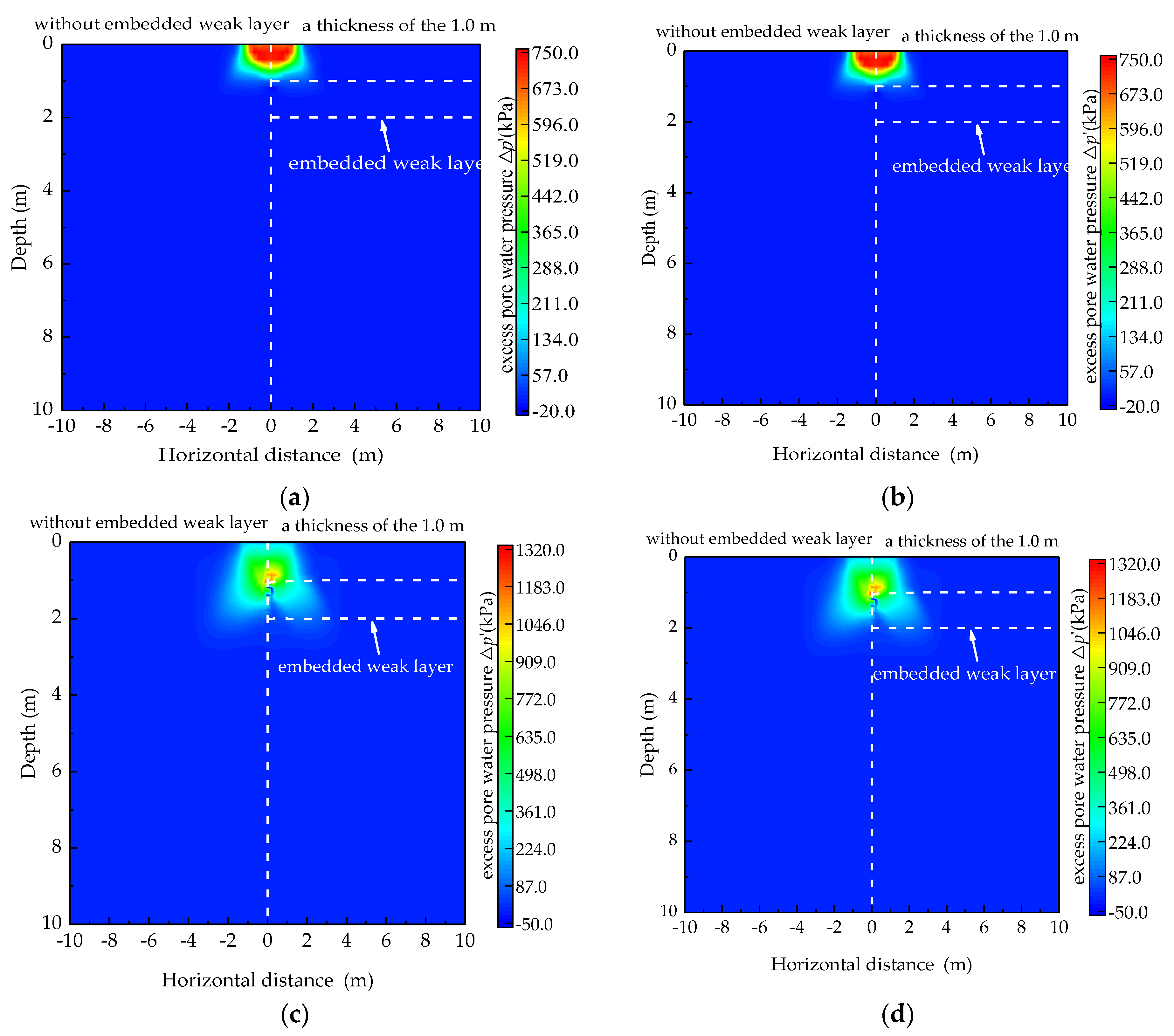
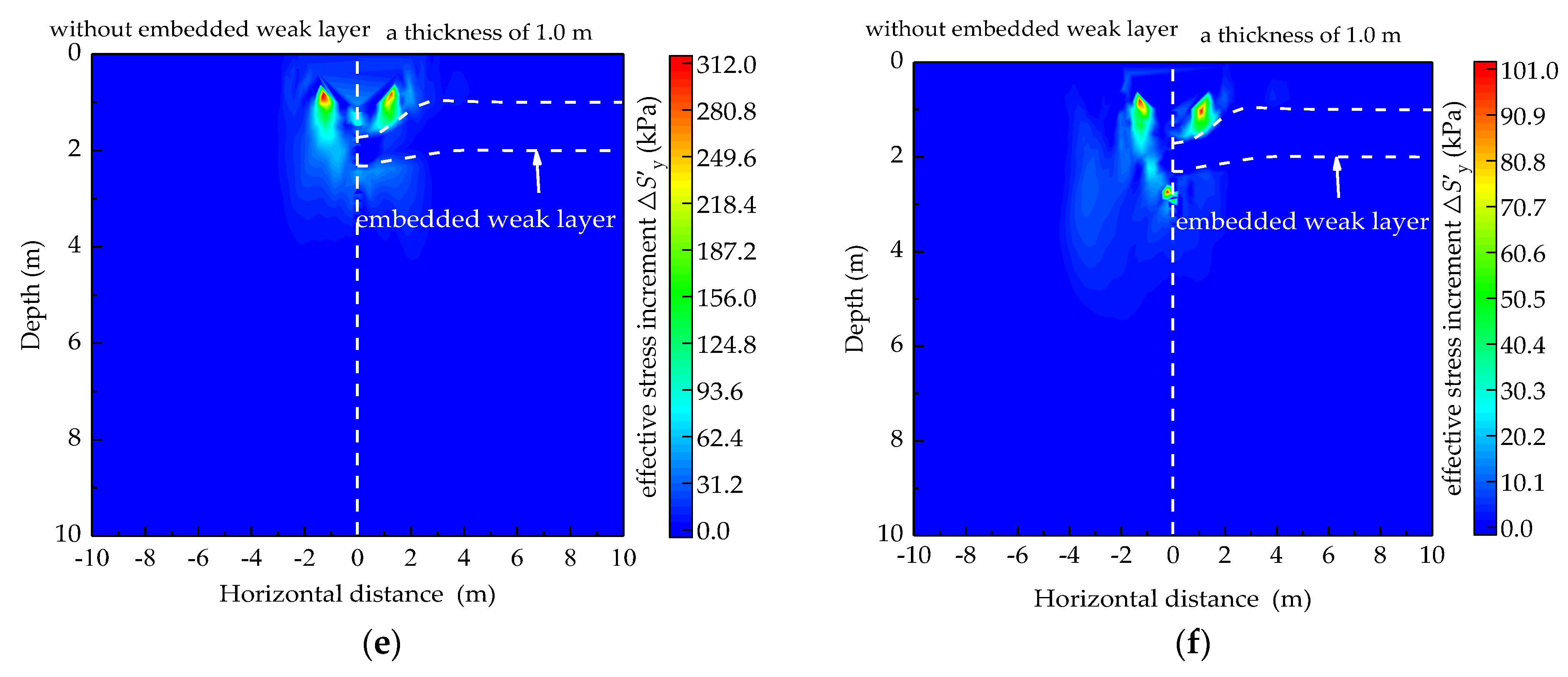
4.1. Improvement Mechanism of Nonhomogeneous Saturated Soil Foundation under DC

To quantify the improvement effect of DC to layered saturated soil foundation, three parameters—effective stress increment ΔS_y’, excess pore water pressure Δp, and the relative degree of reinforcement I_r—proposed by Lee and Gu [14] are used.

$${\mathrm{I}}_{\mathrm{r}}=\frac{{\mathrm{D}}_{\mathrm{r}}-{\mathrm{D}}_{\mathrm{r}0}}{100-{\mathrm{D}}_{\mathrm{r}0}}\times 100\%$$

(11)

where D_r0 and D_r are the relative density of soil before and after DC, respectively. The relative degree of reinforcement I_r is used as it can eliminate the influence of different soil types on the effect of soil improvement [14].

The index of excess pore water pressure ratio Δ${\mathrm{r}}_{\mathrm{u}}$ is defined to quantify the liquefaction potential, which is characterized as:

$$\Delta {\mathrm{r}}_{\mathrm{u}}=\frac{\Delta \mathrm{u}}{{\mathsf{\sigma }}_{\mathrm{s}}^{\text{'}}}$$

(12)

where $\Delta \mathrm{u}$ is the excess pore water pressure generated during DC, and ${\mathsf{\sigma }}_{\mathrm{s}}^{\text{'}}$ is the initial effective stress before implying the dynamic load. Soil liquefaction is supposed to happen as Δr_u reaches 1.0.

In Figure 7, Figure 8 and Figure 9, the evolutions of ΔS_y’, I_r, and Δp in a foundation without weak layers are plotted in the left half of each figure, while those in a foundation with an embedded weak layer with a thickness of 1.0 m are plotted in the right half of each figure. Other parameters in these foundations were set as identical. It is shown that at the first stage of loading (t = 0.01 s), the excess pore water pressure of these two conditions had a similar distribution law. As a continuation of wave propagation (Figure 7b,c), it can be observed that the maximum value of pore pressure bulb occurred nearby the embedded weak layer. For the foundation without a weak layer and with a weak layer, the excess pore water pressure reached the same values of 750 kPa at 0.01 s, which increased to 1500 kPa for the soil with an embedded weak layer and attenuated to 425 kPa for soil without an embedded weak layer at 0.04 s. The dissipation of the excess pore water pressure in the foundation with an embedded weak layer took a long time due to the lower permeability of the weak layer. In contrast, the excess pore water pressure dissipates rapidly in the ground without an weak layer due to the relatively high permeability of soil. It is easy to conclude that the presence of an embedded weak layer has a significant influence on the distribution of the excess pore pressure.

The dynamic reinforcement effect greatly depends on transformation efficiency of the impact load (i.e., effective stress increment), which is finally transferred to the soil skeleton, compacting the soil into a denser state. As shown in Figure 8, at the initial stage of DC, increments of the effective stresses in the foundation with a weak layer were transmitted into the upper soil of weak interlayer, whose distribution is basically in consistent with that of the soil without a weak interlayer. In contrast, the pore water pressure at the same time propagated into the embedded weak layer. It is indicated that the wave characteristic of excess pore pressure and effective stress belong to fast wave and slow compressional wave, respectively [35]. Then, the effective stress wave penetrated into the embedded weak soil layer. However, the increase in effective stress became zero in the embedded weak layer, which was around 215 kPa for soil without an embedded weak layer at the same position. This is because the continuous DC induced the development of pore water pressure in the embedded weak layer of silty clay and the excess pore pressure slowly dissipated, leading the majority of the impact load to be transformed into the excess pore water pressure. Only a small part of the impact load went through the embedded weak interlayer and entered the lower soil. These results indicated that sufficient tamping energy can penetrate into the embedded weak layer, leading the effective stress in the soil below the weak layer increase. At the unloading stage of DC (see Figure 8e,f), the effective stress increment declined and the most of the weak interlayer approached liquefaction.

Figure 9 illustrates the distributions of the relative degree of reinforcement I_r for the grounds with or without a weak layer under DC, varying with time. It can be observed that at the initial stages, there were similar distribution of I_r for the grounds with or without an embedded weak layer. In the continuing process of DC (from t = 0.04 s to t = 1.0 s), the relative degree of reinforcement was about 50% in the range of 0.2 m horizontally and 0.3 m vertically below the weak interlayer. The relative degree of reinforcement I_r in the embedded weak layer was only close to 5%, while the relative degree of reinforcement at the same position without an embedded weak layer was about 50%. There was a 45% difference in the relative reinforcement between these two cases, indicating that larger tamping energy can penetrate through the weak layer to strengthen the lower soil, but has little influence on the improvement effect on the ground with an embedded weak layer.

4.2. Parametric Analysis

A parametric study was performed to analyze the influences of the thickness of the weak interlayer, depth of soft interlayer, tamping energy, and groundwater table on the degree of improvement of soil for single-point tamping. The operational parameters in all cases are shown in

Table 4. Summary of influence factor for foundation with or without an embedded weak layer.

Case	Groundwater Table (m)	Depth of Soft Interlayer (m)	Thickness of Soft Interlayer (m)	Tamping Energy (kN·m)
1	2.0	3.0	0.4	3000
2	2.0	3.0	1.0	3000
3	2.0	3.0	1.6	3000
4	2.0	3.0	2.0	3000
5	2.0	0.4	0.4	3000
6	2.0	1.0	0.4	3000
7	2.0	2.0	0.4	3000
8	2.0	3.0	0.4	3000
9	2.0	3.0	1.0	1000
10	2.0	3.0	1.0	2000
11	2.0	3.0	1.0	3000
12	2.0	3.0	1.0	4000
13	3.0	3.0	1.0	3000
14	4.0	3.0	1.0	3000
15	5.0	3.0	1.0	3000

.

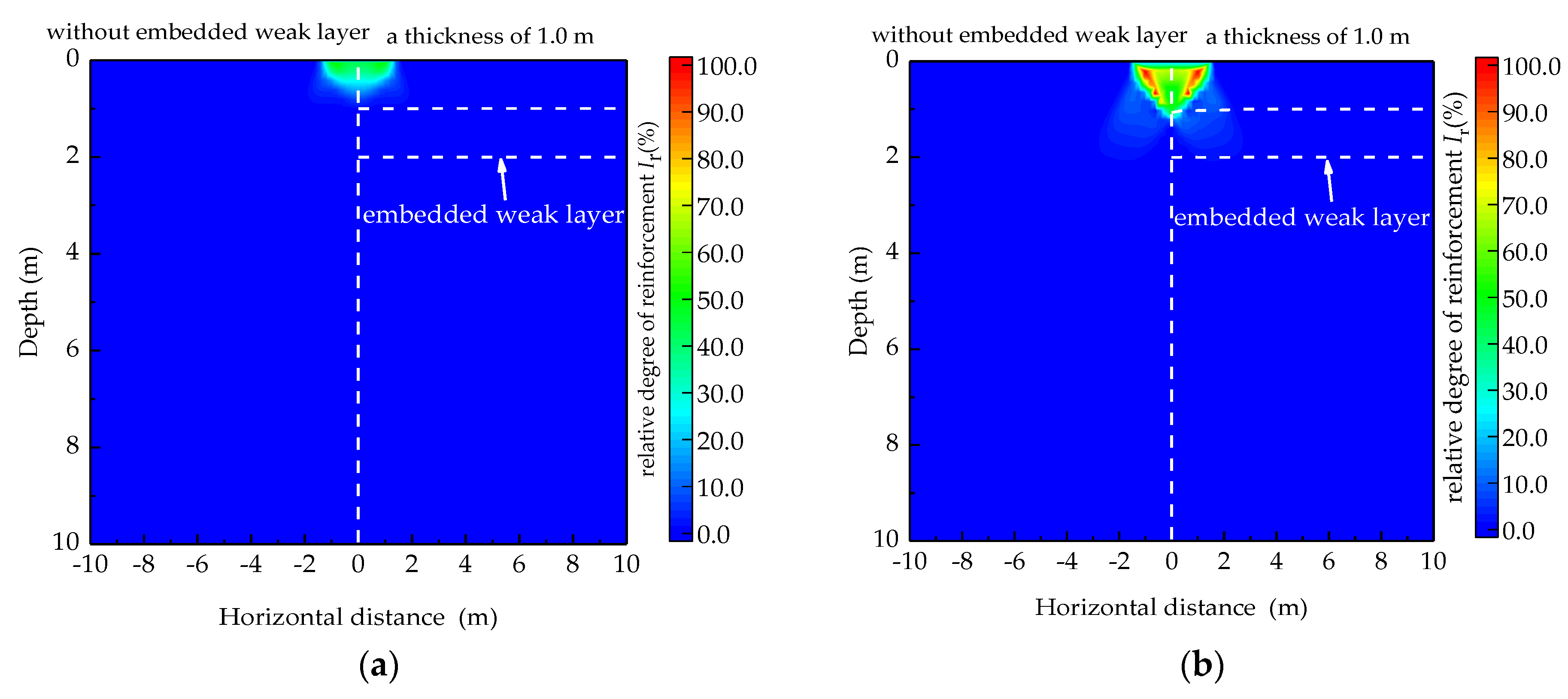
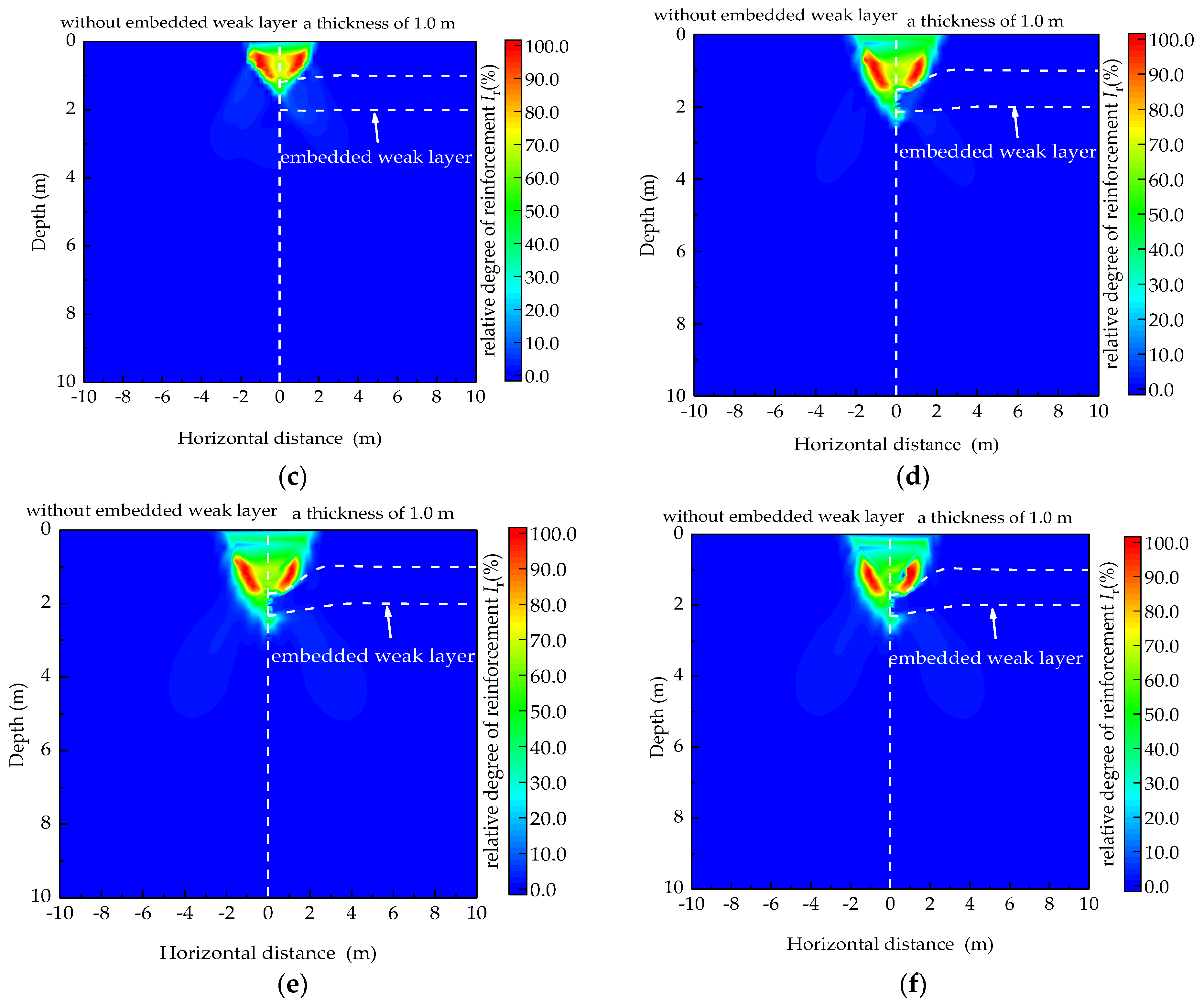
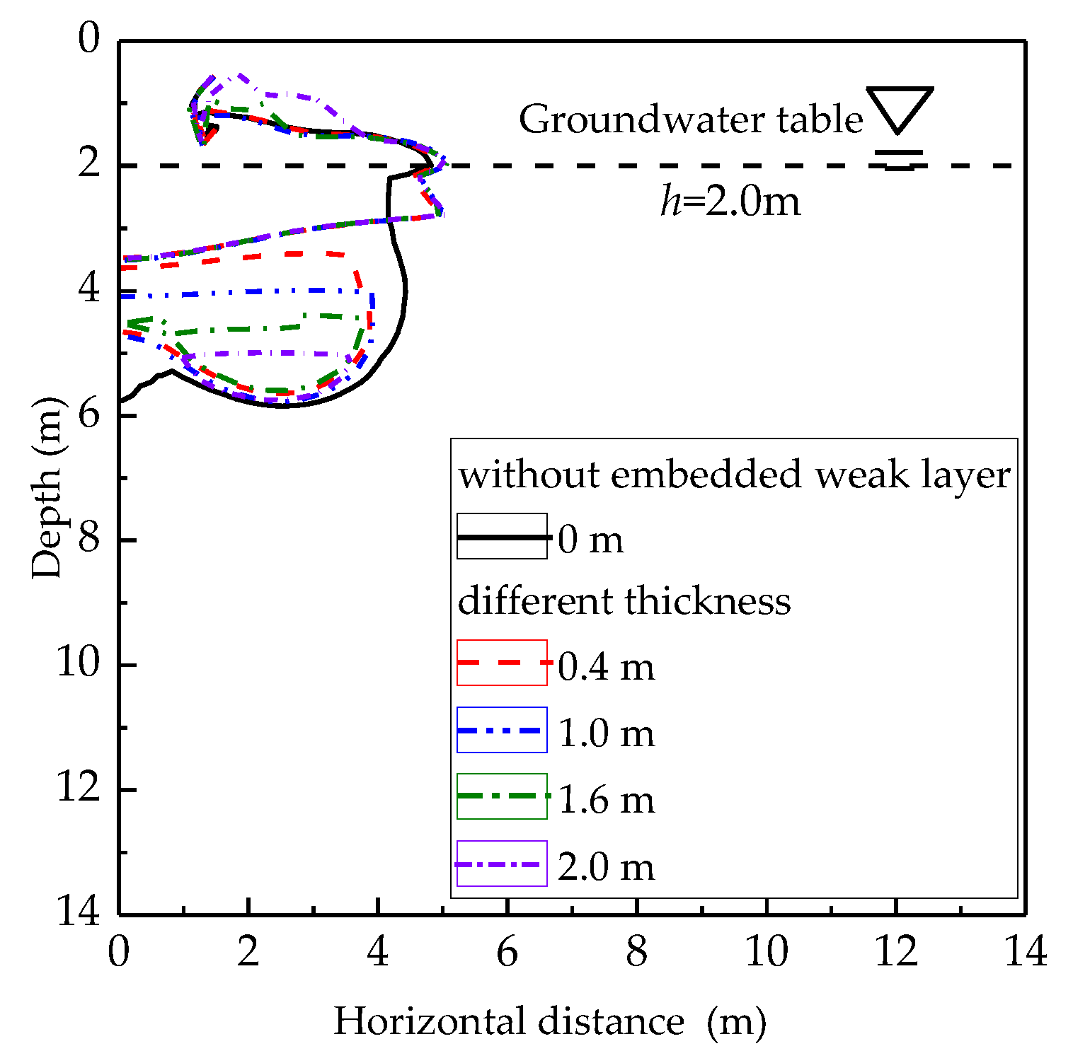
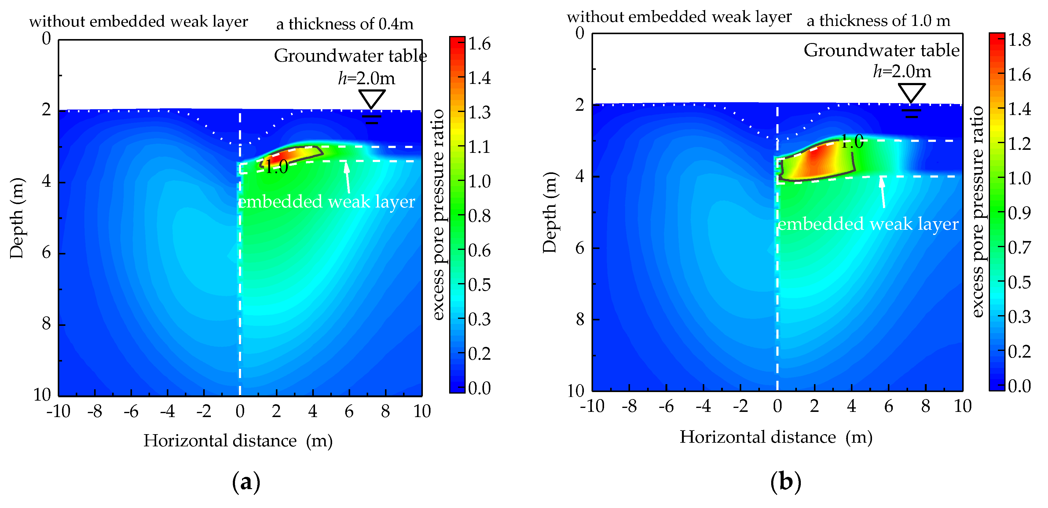
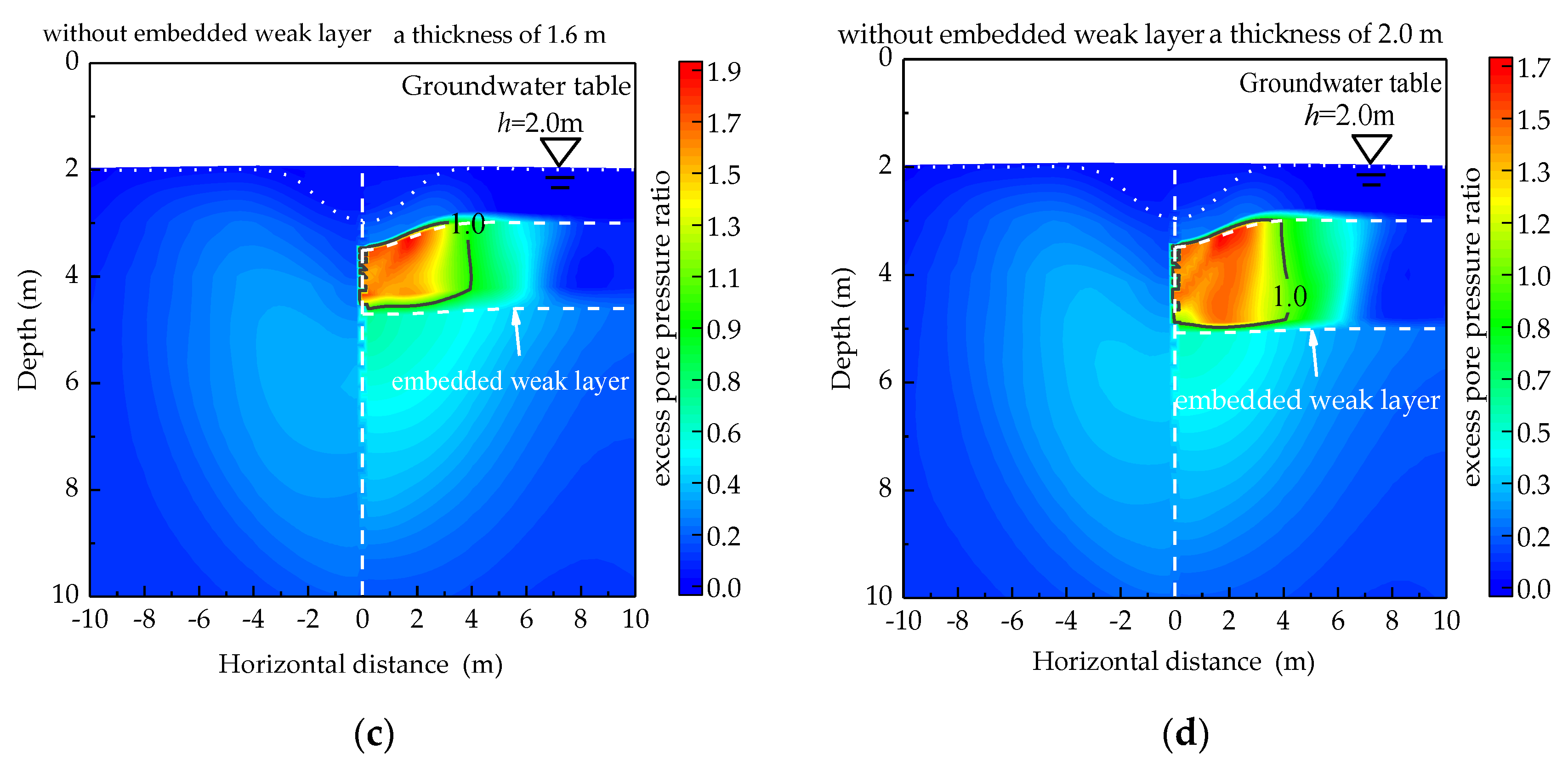
4.2.1. Influences of Thickness of the Embedded Weak Layer

The numerical simulation of DC was performed with the thickness of soft interlayer ranging from 0.4 to 2.0 m to investigate the effect of the thickness of the weak interlayer on the reinforcement effect of soft soil stratum and the rising of pore water pressure in embedded weak layer. The left half of each figure presents the foundation without an embedded weak layer, while the right half represents the foundation with an embedded weak layer (see cases 1 to 4 in Table 4).

Figure 10 shows the distribution of I_r in grounds with a weak layer of different thicknesses. The white curve represents the zone of I_r = 7.7%. Figure 11 describes cloud lines of I_r = 7.7% for different thickness of embedded weak layer. It can be found that the zone of I_r = 7.7% of the soil above the weak layer basically did not change with the thickness of the interlayer, whereas the reinforcement range of the soil below the weak layer decreased with the increase of the thickness of the interlayer. In ground with a thin interlayer (Figure 10a,b), the tamping energy can penetrate through the embedded weak layer into the underlying soil. However, as the embedded weak layer became thicker, the improvement effect to the lower soil became weakened, indicating that the embedded weak layer prevented the transmission of tamping energy.

Figure 12 shows the distribution of the excess pore water pressure ratio in grounds with embedded weak layer of different thickness. It can be seen that the liquefied zone (Δr_u < 1.0) was mainly in the embedded weak layer, and the range of liquefied zone increased with the increase of the thickness of the embedded weak layer. The results indicate that the excess pore pressure in the ground with an embedded weak layer accumulated as DC continued, resulting in failure of effective reinforcement to the embedded weak layer. Moreover, the maximum excess pore pressure ratio of the upper soil without a weak interlayer was generally less than 0.2, indicating that the pore pressure dissipated quickly, and a better reinforcement effect was obtained. The excess pore water pressure ratio Δr_u within the soil below the embedded weak layer was greater than that in the ground without an embedded weak layer at the same depth. It can be concluded that the presence of an embedded weak layer makes the pore water cannot be drained in time, resulting in a continuous accumulation of pore water pressure.

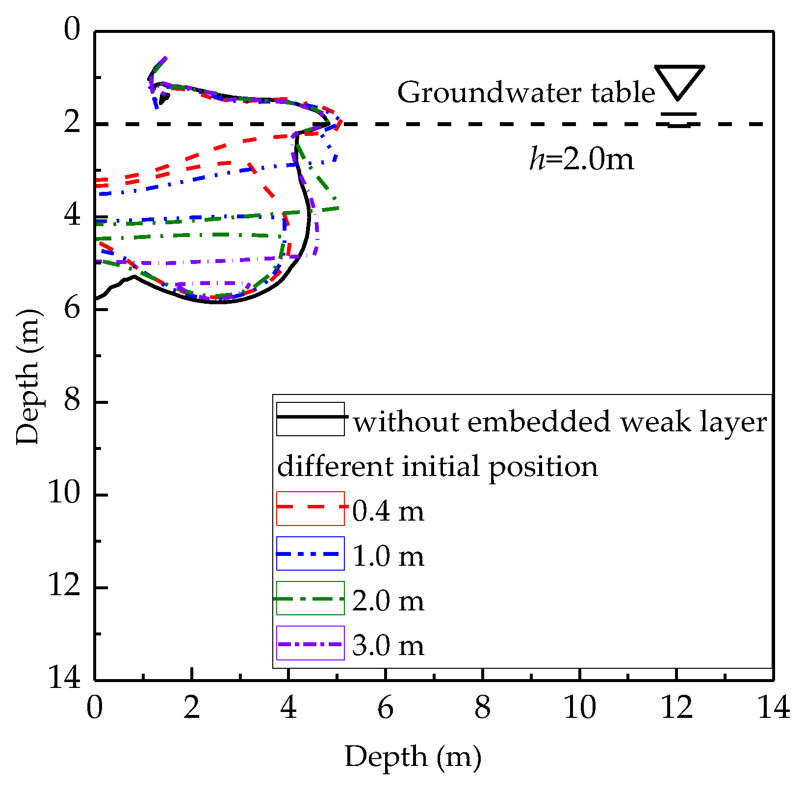
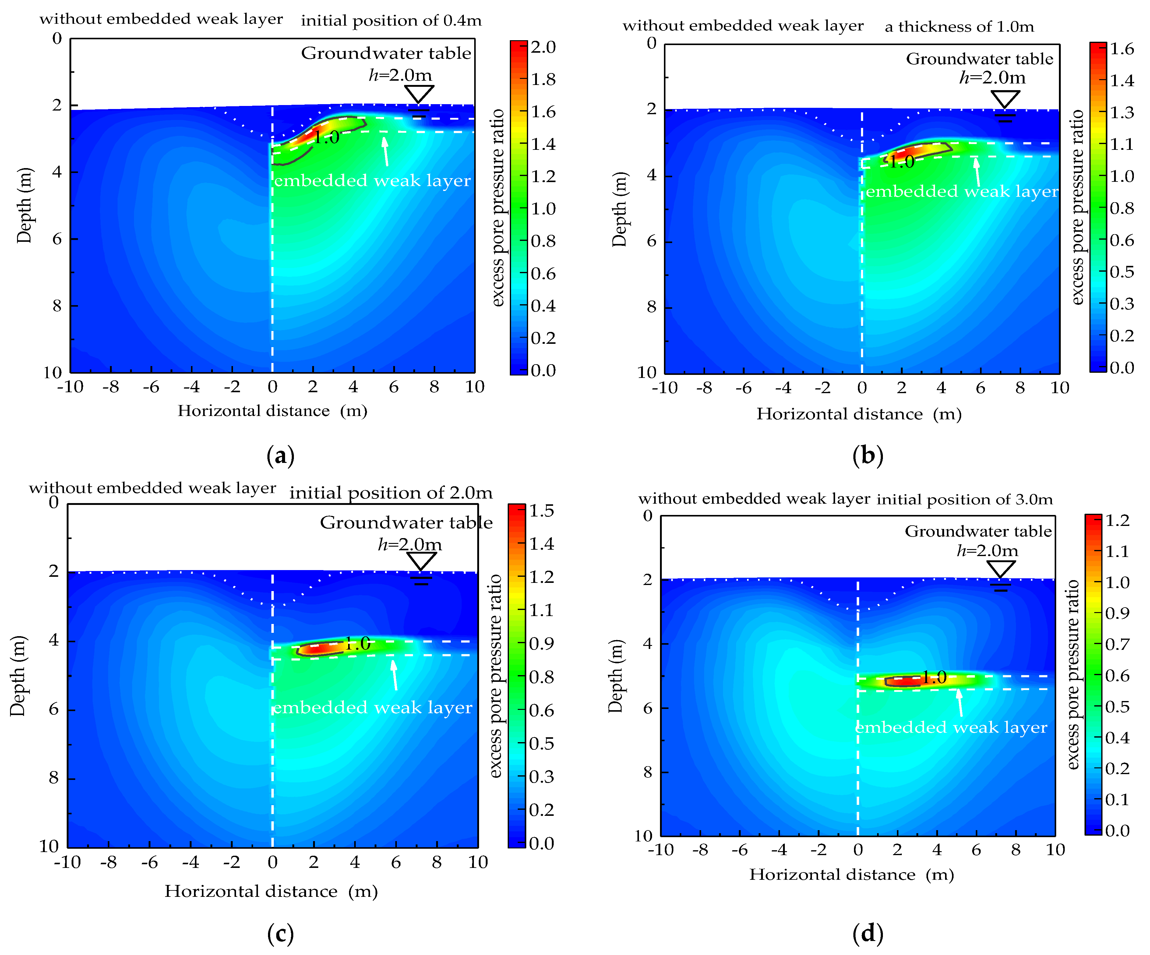
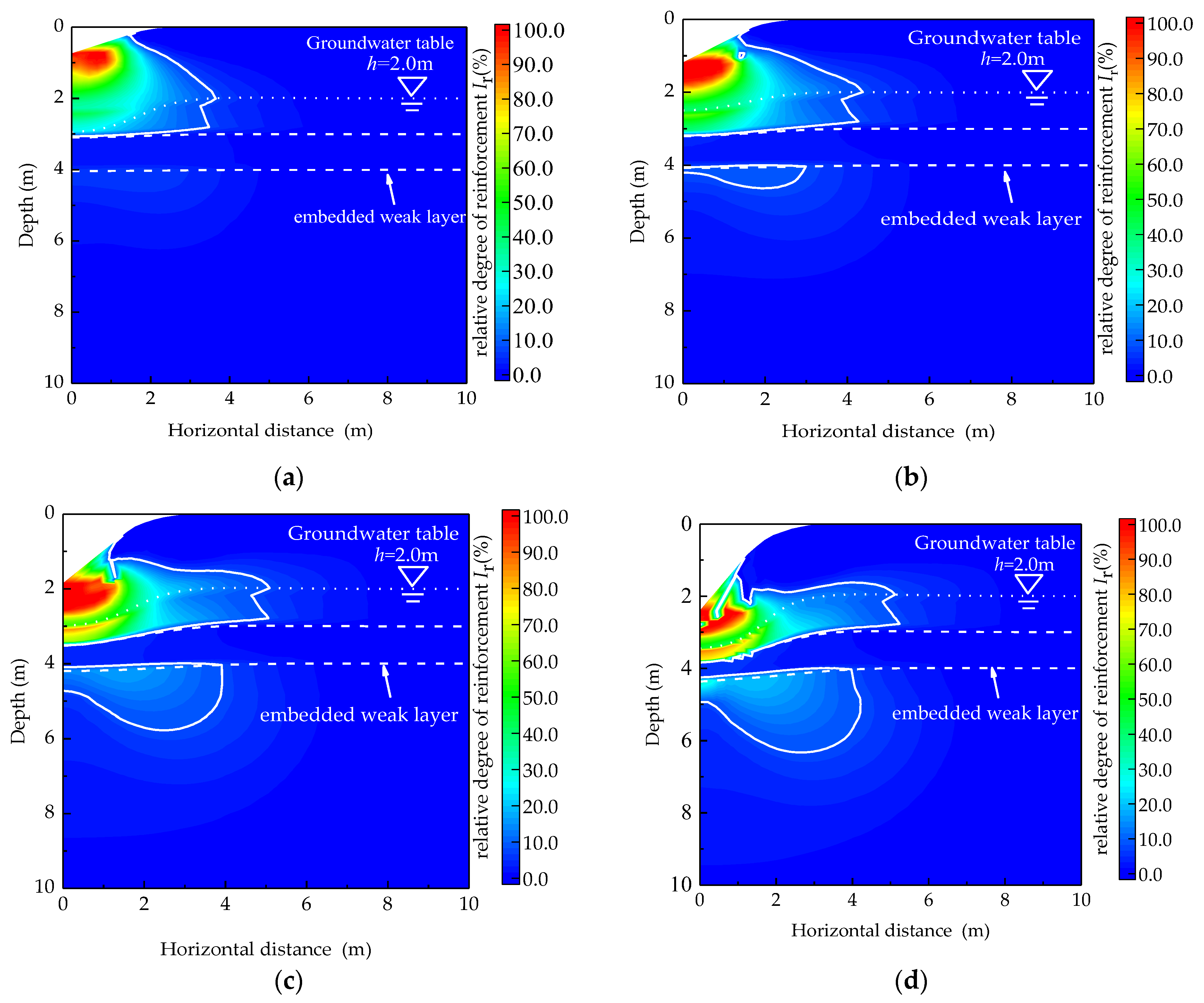
4.2.2. Influences of Depth of the Embedded Weak Layer

In the numerical simulations, the depth of the embedded weak layer ranged from 0.4 to 3.0 m to investigate its influences on the improvement effect of DC to the saturated ground. The left half of each figure presents the ground without a weak layer, while the right half represents the ground with an embedded weak layer (see cases 5 to 8 in Table 4).

The distributions of I_r in grounds with an embedded weak layer at different initial depths are shown in Figure 13. The white curve represents the zone of I_r = 7.7%. Figure 14 shows cloud lines of I_r = 7.7% for different initial depths of soft interlayers. It can be found that the relative reinforcement degree to the embedded weak layer in the ground was around 0. It was also noted that as the depth of the embedded weak layer went down, the zone of compacted soil above the weak layer increased. However, the reinforcement effect to the soil below the weak interlayer decreased as the initial depth of the soft interlayer moved deeper. This is because that as the weak interlayer located deeper, the zone of the upper soil became thicker so that the tamping energy that was transferred into the weak interlayer decreased; thus, the underlying soil was less compacted.

Figure 15 shows that the zone with high excess pore pressure was mainly concentrated in the embedded weak layer and the excess pore pressure dissipated slowly in this layer, which directly affected the reinforcement effect. Specifically, by analyzing the pore pressure distribution, the excess pore pressure ratio in soil above the weak layer was the lowest and did not change with the depth of the embedded weak layer, while that in the embedded weak layer was the highest. The excess pore pressure cannot dissipate in time in the weak layer, in which the maximum value of the excess pore pressure ratio decreased gradually as the embedded weak layer became deeper. Due to the influence of the embedded weak layer, the pore water in the soil below the weak interlayer could not be discharged in time, leading to a higher excess pore pressure ratio (or less compaction) than that in the ground without an embedded weak layer at the same depth.

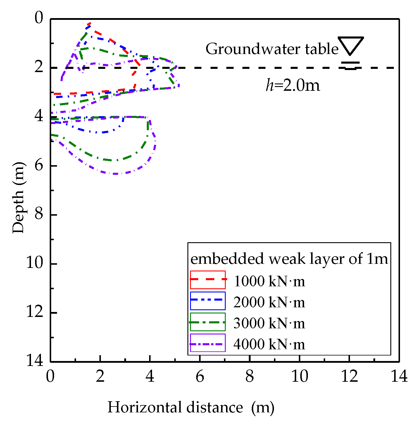
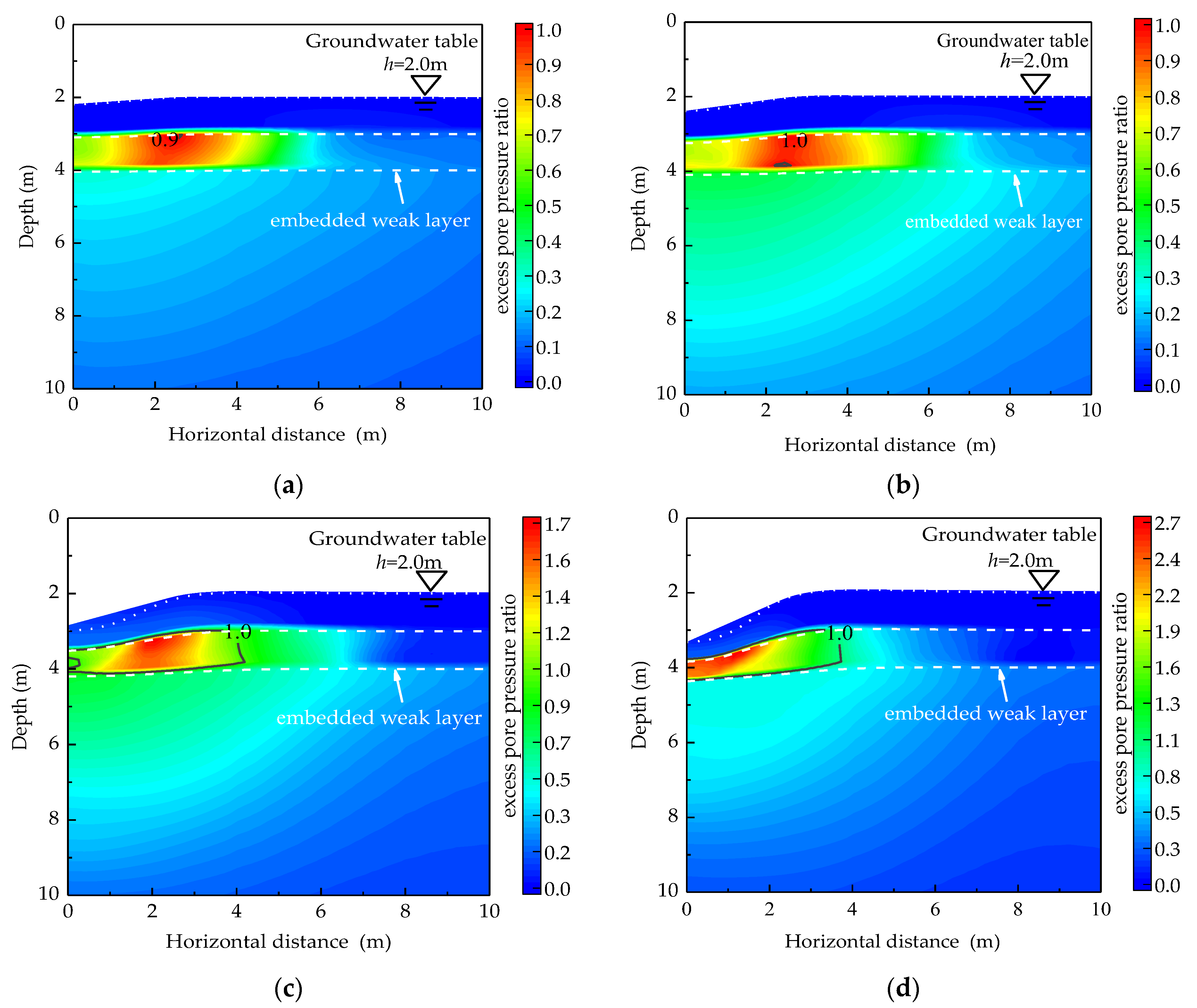
4.2.3. Effect of Tamping Energy

In order to investigate how the tamping energy influences the dynamic compaction effects to saturated ground with a weak interlayer, the tamping energy of DC ranged from 1000 kN·m to 4000 kN·m t in the numerical simulations. The left half of each figure presents the foundation without an embedded weak layer, while the right half represents the foundation with an embedded weak layer (see cases 9 to 12 in Table 4).

Figure 16 and Figure 17 show that as the tamping energy increased, the zone of I_r = 7.7% below the embedded weak layer increased significantly. The soil above the embedded weak layer experienced the largest compaction. The relative degree of reinforcement in the embedded weak layer was close to 0. It is proved that a further increase in the tamping energy has little effect on reinforcement effect in the embedded weak layer. It should be noted that I_r below the embedded weak layer was only marginally affected by tamping energy while it is 1000 kN·m, which suggests that there was not a significant change of reinforcement effect in the embedded weak layer by small tamping energy. However, the reinforcement effect below the embedded weak layer was improved obviously when the tamping energy increased to 4000 kN·m. The reinforcement effect could be improved obviously by properly increasing tamping energy.

Figure 18 shows that the excess pore pressure ratio in the upper soil of the weak layer was close to 0 after 10 blows due to its high permeability, the soil in which the layer was effectively reinforced. For the embedded weak layer, the dissipation of pore pressure was not obvious, and the excess pore pressure ratio reached its maximum values, increasing significantly with increases of the tamping energy. If the tamping energy was too large, the dissipation of excess pore pressure of soil would be incomplete, especially in the soft interlayer foundation with high mud content. In other words, the tamping energy should not be too large, so as to avoid the complete destruction of soil structure or the formation of “rubber soil”. For the soil below the weak layer, the residual excess pore water pressure still remained at a high level, which required a certain time to dissipate due to the existence of the embedded weak layer. This prevented the further development of the reinforcement effect at depths below the weak layer.

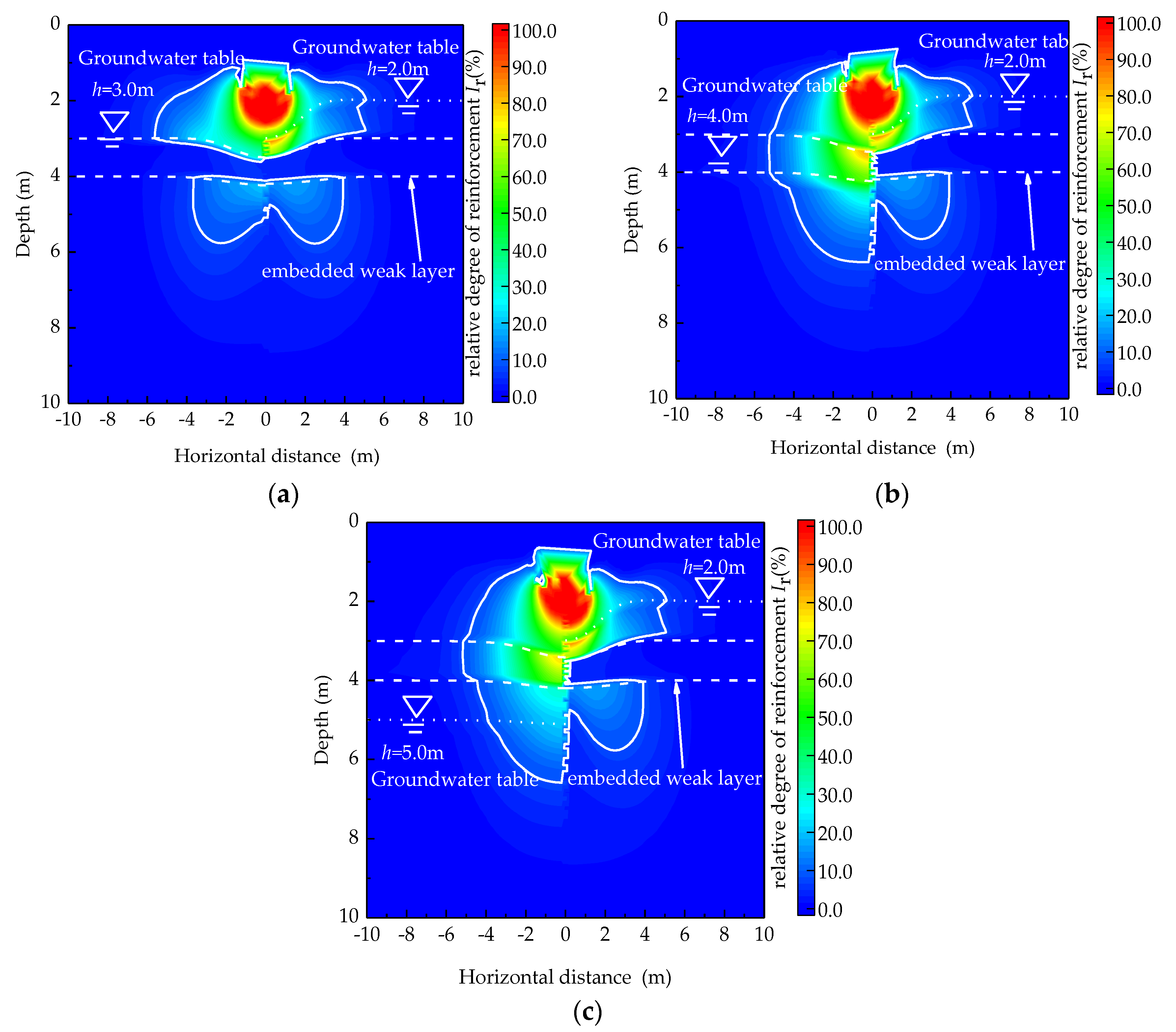
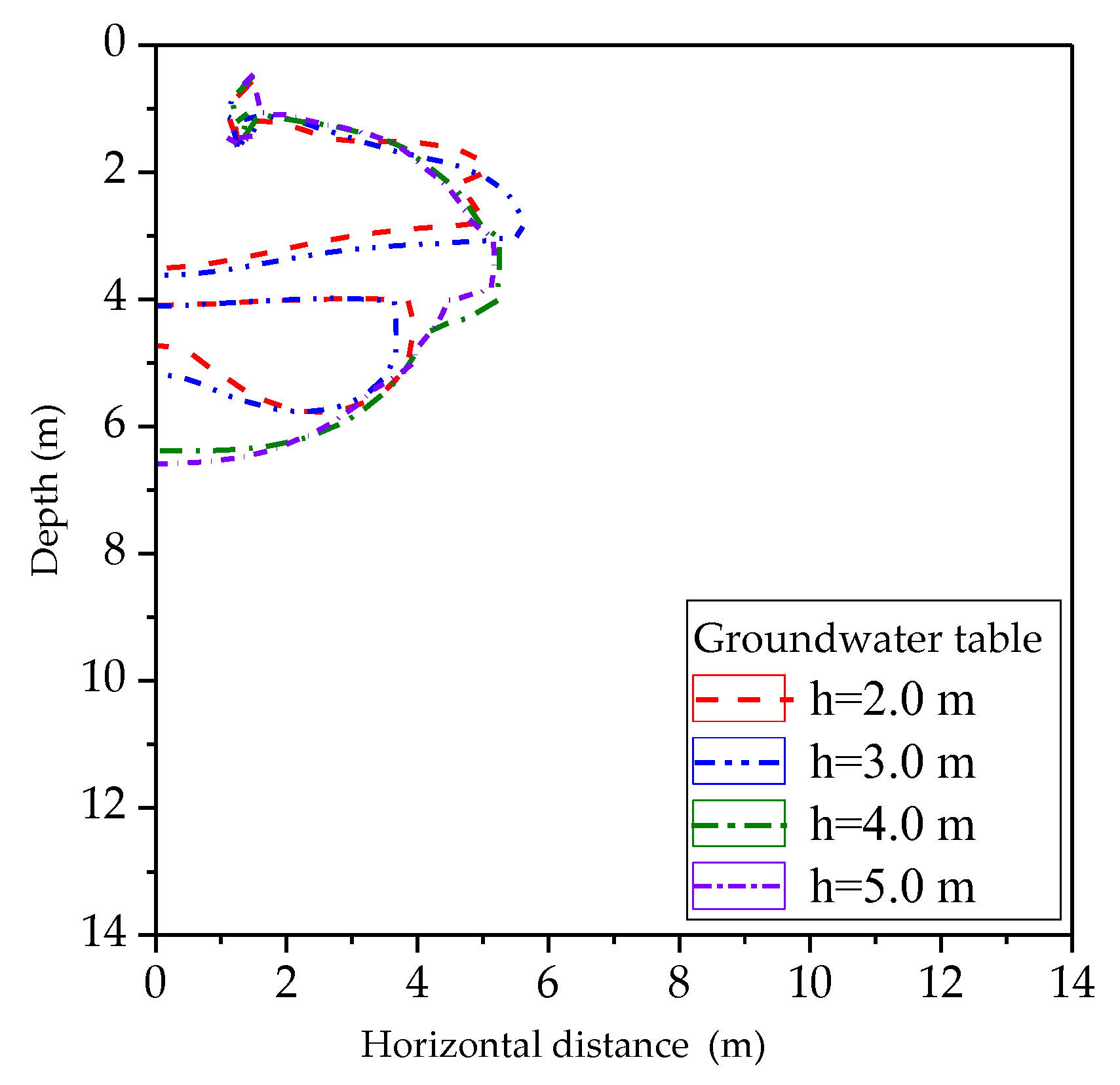
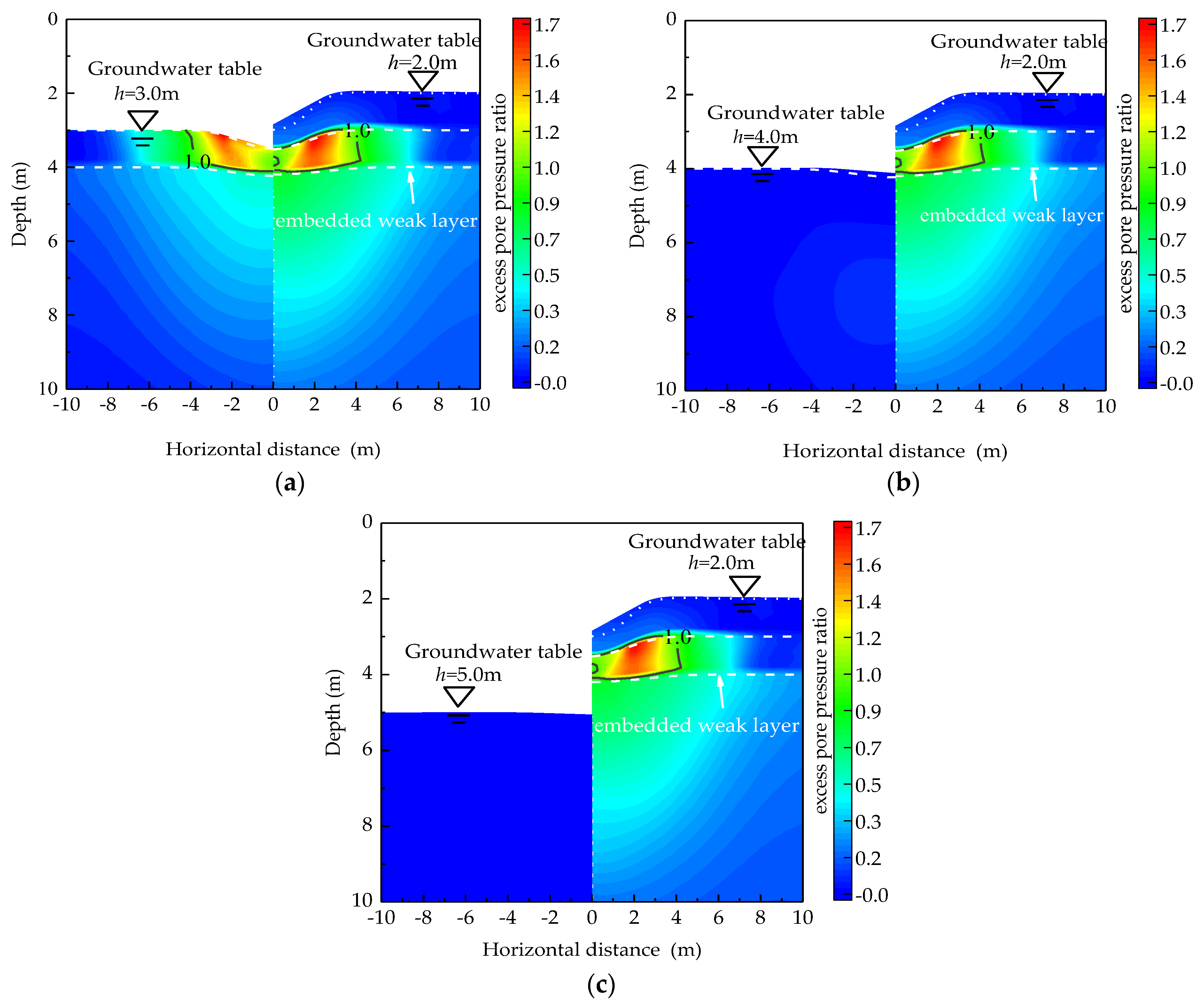
4.2.4. Effect of Groundwater Table

Influences of the groundwater table on the compaction effect of DC to the grounds were investigated by performing numerical simulations with groundwater table ranging from 2 to 5 m. The right half of each figure presents the foundation with groundwater table of 2 m, while the left half represents the foundation for different groundwater table (cases 11 and 13–15 in Table 3).

It can be seen from Figure 19 and Figure 20 that, with decreases of the groundwater table, the effective reinforcement range of the embedded weak layer and soil beneath it expanded significantly, and the maximum relative reinforcement degree was mainly concentrated in the upper soil of the weak layer. When the groundwater table dropped to the depth of the embedded weak layer, the reinforcement effect of the embedded weak layer and the soil beneath it did not vary any more.

Figure 21 shows comparisons of excess pore pressure ratios in the embedded weak layer in grounds with different levels of groundwater after DC. It is found that when the level of groundwater was above the weak layer, the excess pore pressure in the embedded weak layer increased significantly, and this influence decreased as the groundwater table decreased from h = 2.0 m to h = 3.0 m. While the groundwater table was below the bottom of the weak layer (e.g., h = 4.0 m and h = 5.0 m), the excess pore pressure ratio in the weak layer was 0. The results indicate that lowering of the groundwater table can significantly improve the reinforcement effect of DC to the embedded weak layer and the soil beneath it. It should be mentioned that DC is better carried out until the groundwater is lowered below the designed depth, especially in grounds with shallow weak layers.

5. Conclusions

In this paper, the improvement mechanism of DC in layered saturated soil ground was investigated by performing fluid–solid coupling simulations. Major conclusions are drawn as follows:

1. The Dual-Phase Coupling Method in Abaqus can well reflect the development law of excess pore water pressure and the reinforcement effects of DC in saturated grounds with a weak soil layer.

2. The embedment depth and thickness of the weak layer are important factors affecting the effective reinforcement depth. For grounds with a weak layer of a thin thickness and at shallow depths, sufficient tamping energy can penetrate through the soft interlayer, thus reinforcing the lower part of the soft interlayer as long as the transverse range of the liquefied zone is not large. While the weak soil layer is thick and buried deep, the effective reinforcement depth of DC is hard to exceed the embedded weak layer.

3. Improving the tamping energy may enlarge the range of liquefied zone (ΔR_u > 1.0) in the soft interlayer. However, excessive tamping energy can lead to great excessive excess pore water pressure in the weak embedded layer, which may lead to the formation of “rubber soil”.

4. To achieve a better compaction effect during DC, the groundwater table should be lowered by dewatering or adding a drainage layer (e.g., a layer of coarse-grained material) to shorten the drainage distance between the ground surface and the groundwater.

References

1. Hasheminezhad, A.; Bahadori, H. Seismic response of shallow foundations over liquefiable soils improved by deep soil mixing columns. Comput. Geotech. 2019, 110, 251–273. [Google Scholar] [CrossRef]
2. Bahadori, H.; Farzalizadeh, R.; Barghi, A.; Hasheminezhad, A. A comparative study between gravel and rubber drainage columns for mitigation of liquefaction hazards. J. Rock Mech. Geotech. Eng. 2018, 10, 924–934. [Google Scholar] [CrossRef]
3. Bahadori, H.; Motamedi, H.; Hasheminezhad, A.; Motamed, R. Shaking table tests on shallow foundations over geocomposite and geogrid-reinforced liquefiable soils. Soil Dyn. Earthq. Eng. 2020, 128, 105896. [Google Scholar] [CrossRef]
4. Jun, C.A.I.; Zhang, J.; Guangyin, D.U.; Han, X.I.A. Application of the dynamic compaction method for ground improvement of collapsible loess in Qinhai. Teknik Dergi 2022, 33, 11455–11472. [Google Scholar]
5. Majik, R.K.; Savoikar, P.P. Ground modification techniques for deep soft soils sites in Goa region. In Ground Improvement and Reinforced Soil Structures; Springer: Singapore, 2022; pp. 409–421. [Google Scholar]
6. Bo, M.W.; Na, Y.M.; Arulrajah, A.; Chang, M.F. Densification of granular soil by dynamic compaction. Proc. Inst. Civ. Eng. Ground Improv. 2009, 162, 121–132. [Google Scholar] [CrossRef]
7. Feng, S.J.; Tan, K.; Shui, W.H.; Zhang, Y. Densification of desert sands by high energy dynamic compaction. Eng. Geol. 2013, 157, 48–54. [Google Scholar] [CrossRef]
8. Shenthan, T.; Nashed, R.; Thevanayagam, S.; Martin, G.R. Liquefaction mitigation in silty soils using composite stone columns and dynamic compaction. Earthq. Eng. Eng. Vib. 2004, 3, 39–50. [Google Scholar] [CrossRef]
9. Cao, Y.C.; Wang, W.T. Seabed ground improvement in coastal reclamation area by heavy tamping after rockfilling displacement. Mar. Georesources Geotechnol. 2007, 25, 1–14. [Google Scholar] [CrossRef]
10. Mayne, P.W.; Jones, J.S., Jr.; Dumas, J.C. Ground response to dynamic compaction. J. Geotech. Eng. 1984, 110, 757–774. [Google Scholar] [CrossRef]
11. Nashed, R. Liquefaction Mitigation Of Silty Soils Using Dynamic Compaction; State University of New York at Buffalo: New York, NY, USA, 2006. [Google Scholar]
12. Feng, S.J.; Shui, W.H.; Tan, K.; Gao, L.Y.; He, L.J. Field evaluation of dynamic compaction on granular deposits. J. Perform. Constr. Facil. 2011, 25, 241–249. [Google Scholar] [CrossRef]
13. Feng, S.J.; Du, F.L.; Shi, Z.M.; Shui, W.H.; Tan, K. Field study on the reinforcement of collapsible loess using dynamic compaction. Eng. Geol. 2015, 185, 105–115. [Google Scholar] [CrossRef]
14. Lee, F.H.; Gu, Q. Method for estimating dynamic compaction effect on sand. J. Geotech. Geoenviron. Eng. 2004, 130, 139–152. [Google Scholar] [CrossRef]
15. Wang, W.; Chen, J.J.; Wang, J.H. Estimation method for ground deformation of granular soils caused by dynamic compaction. Soil Dyn. Earthq. Eng. 2017, 92, 266–278. [Google Scholar] [CrossRef]
16. Dou, J.; Chen, J.; Wang, W. Method for estimating the degree of improvement in soil between adjacent tamping locations under dynamic compaction. Int. J. Geomech. 2019, 19, 04019134. [Google Scholar] [CrossRef]
17. Zhou, C.; Jiang, H.; Yao, Z.; Li, H.; Yang, C.; Chen, L.; Geng, X. Evaluation of dynamic compaction to improve saturated foundation based on the fluid-solid coupled method with soil cap model. Comput. Geotech. 2020, 125, 103686. [Google Scholar] [CrossRef]
18. Zhou, C.; Yang, C.; Qi, H.; Yao, K.; Yao, Z.; Wang, K.; Ji, P.; Li, H. Evaluation on improvement zone of foundation after dynamic compaction. Appl. Sci. 2021, 11, 2156. [Google Scholar] [CrossRef]
19. Perucho, A.; Olalla, C. Dynamic consolidation of a saturated plastic clayey fill. Proc. Inst. Civ. Eng. Ground Improv. 2006, 10, 55–68. [Google Scholar] [CrossRef]
20. Feng, S.J.; Lu, S.F.; Shi, Z.M.; Shui, W.H. Densification of loosely deposited soft soils using the combined consolidation method. Eng. Geol. 2014, 181, 169–179. [Google Scholar] [CrossRef]
21. Feng, S.J.; Du, F.L.; Chen, H.X.; Mao, J.Z. Centrifuge modeling of preloading consolidation and dynamic compaction in treating dredged soil. Eng. Geol. 2017, 226, 161–171. [Google Scholar] [CrossRef]
22. Jia, M.; Cheng, J.; Liu, B.; Ma, G. Model tests of the influence of ground water level on dynamic compaction. Bull. Eng. Geol. Environ. 2021, 80, 3065–3078. [Google Scholar] [CrossRef]
23. Abdizadeh, D.; Pakbaz, M.S.; Nadi, B. Numerical modeling of lateral dynamic compaction on the slope in dry sand. KSCE J. Civ. Eng. 2021, 25, 398–403. [Google Scholar] [CrossRef]
24. Yao, K.; Yao, Z.Y.; Song, X.G.; Shang, Q.S. Test study of pore water pressure during dynamic compaction at the subgrade of highway in the Yellow River Flood Area. In Advanced Materials Research; Trans Tech Publications Ltd.: Wollerau, Switzerland, 2012; Volume 374, pp. 436–439. [Google Scholar]
25. Yao, K.; Rong, Y.; Yao, Z.; Shi, C.; Yang, C.; Chen, L.; Zhang, B.; Jiang, H. Effect of water level on dynamic compaction in silty ground of Yellow River alluvial plain. Arab. J. Geosci. 2022, 15, 1–16. [Google Scholar] [CrossRef]
26. Chen, X.Y.; Guo, B.X.; Xie, Y.L.; Ma, Y.F. Field Test on influencing factors and vibration law of dynamic compaction for sand foundation. Pet. Eng. Constr. 2016, 42, 64–68. (In Chinese) [Google Scholar]
27. Song, X.G.; Sun, R.S.; Dong, H.; Liu, X.L.; Wang, K.; Bo, M.; Sang, X.R. Field test of foundation dynamic compaction about soft interlayer structure in yellow river flood area. J. Archit. Civ. Eng. 2018, 35, 26–32. (In Chinese) [Google Scholar]
28. Jia, M.; Zhao, Y.; Zhou, X. Field studies of dynamic compaction on marine deposits. Mar. Georesources Geotechnol. 2016, 34, 313–320. [Google Scholar] [CrossRef]
29. Ye, F.; Goh, S.; Lee, F. A method to solve biot’s uu formulation for soil dynamics applications using the abaqus/explicit platform. Numer. Methods Geotech. Eng. 2010, 417–422. [Google Scholar]
30. Ye, F.; Goh, S.H.; Lee, F.H. Dual-phase coupled u–U analysis of wave propagation in saturated porous media using a commercial code. Comput. Geotech. 2014, 55, 316–329. [Google Scholar] [CrossRef]
31. Zhou, C.; Yao, K.; Rong, Y.; Lee, F.H.; Zhang, D.; Jiang, H.; Yang, C.; Yao, Z.; Chen, L. Numerical investigation on zone of improvement for dynamic compaction of sandy ground with high groundwater table. Acta Geotech. 2022, 1–15. [Google Scholar] [CrossRef]
32. Yao, Z.; Zhou, C.; Lin, Q.; Yao, K.; Satchithananthan, U.; Lee, F.H.; Wang, S. Effect of dynamic compaction by multi-point tamping on the densification of sandy soil. Comput. Geotech. 2022, 151, 104949. [Google Scholar] [CrossRef]
33. Helwany, S. Applied Soil Mechanics with ABAQUS Applications; John Wiley & Sons: Hoboken, NJ, USA, 2007. [Google Scholar]
34. Miao, L.; Chen, G.; Hong, Z. Application of dynamic compaction in highway: A case study. Geotech. Geol. Eng. 2006, 24, 91–99. [Google Scholar] [CrossRef]
35. Yi, J.T.; Zhang, L.; Ye, F.J.; Goh, S.H. One-dimensional transient wave propagation in a dry overlying saturated ground. KSCE J. Civ. Eng. 2019, 23, 4297–4310. [Google Scholar] [CrossRef]
Figure 1. Failure surface of the Cap model in p–q plane [33].
Applsci 12 09770 g001
Figure 2. Excess pore water pressure versus time. (a) 1500 kN·m; (b) 2500 kN·m [17].
Applsci 12 09770 g002
Figure 3. Comparison with the field results for the case of 1500 kN·m tamping energy. (a) Excess pore water pressure versus soil depth; (b) Lateral displacement versus soil depth.
Applsci 12 09770 g003
Figure 4. Comparison with the field results for the case of 2500 kN·m tamping energy [17]. (a) Excess pore water pressure versus soil depth; (b) Lateral displacement versus soil depth.
Applsci 12 09770 g004
Figure 5. The finite element model of foundation with embedded weak layer.
Applsci 12 09770 g005
Figure 6. Comparison results of relative density [26].
Applsci 12 09770 g006
Figure 7. Distribution of Δp in grounds with and without a weak layer during DC. (a) t = 0.01 s; (b) t = 0.02 s; (c) t = 0.04 s; (d) t = 0.1 s.
Applsci 12 09770 g007
Figure 8. Distributions of ΔS’y in grounds with or without an embedded weak layer during DC. (a) t = 0.01 s; (b) t = 0.02 s; (c) t = 0.04 s; (d) t = 0.1 s; (e) t = 0.2 s; (f) t = 2.0 s.
Applsci 12 09770 g008aApplsci 12 09770 g008b
Figure 9. Distributions of Ir of foundation with or without an embedded weak layer during the DC. (a) t = 0.01 s; (b) t = 0.02 s; (c) t = 0.04 s; (d) t = 0.1 s; (e) t = 0.2 s; (f) t = 1 s.
Applsci 12 09770 g009aApplsci 12 09770 g009b
Figure 10. Distributions of Ir in grounds with different thickness of embedded weak layer. (a) 0.4 m; (b) 1 m; (c) 1.6 m; (d) 2.0 m.
Applsci 12 09770 g010
Figure 11. Cloud lines of Ir = 7.7% for different thickness of embedded weak layer.
Applsci 12 09770 g011
Figure 12. Distributions of excess pore water pressure ratio in grounds with embedded weak layers of different thicknesses. (a) 0.4 m; (b) 1 m; (c) 1.6 m; (d) 2.0 m.
Applsci 12 09770 g012aApplsci 12 09770 g012b
Figure 13. Cloud charts of Ir for different initial position of embedded weak layer. (a) 0.4 m; (b) 1 m; (c) 2.0 m; (d) 3.0 m.
Applsci 12 09770 g013aApplsci 12 09770 g013b
Figure 14. Cloud lines of Ir = 7.7% for different initial position of soft interlayers.
Applsci 12 09770 g014
Figure 15. Distributions of excess pore water pressure ratio in grounds with weak interlayer of different initial position. (a) 0.4 m; (b) 1 m; (c) 2.0 m; (d) 3.0 m.
Applsci 12 09770 g015
Figure 16. Distributions of Ir of embedded weak layer for different tamping energy. (a) 1000 kN·m; (b) 2000 kN·m; (c) 3000 kN·m; (d) 4000 kN·m.
Applsci 12 09770 g016
Figure 17. Cloud lines of Ir = 7.7% of embedded weak layer for different tamping energy.
Applsci 12 09770 g017
Figure 18. Cloud charts of excess pore water pressure ratio of embedded weak layer for different drop energy. (a) 1000 kN·m; (b) 2000 kN·m; (c) 3000 kN·m; (d) 4000 kN·m.
Applsci 12 09770 g018
Figure 19. Distributions of Ir in grounds with different levels of groundwater. (a) precipitation depth of 3 m; (b) precipitation depth of 4 m; (c) precipitation depth of 5 m.
Applsci 12 09770 g019
Figure 20. Cloud lines of Ir = 7.7% in grounds with different levels of groundwater.
Applsci 12 09770 g020
Figure 21. Distributions of excess pore water pressure ratio in grounds of different levels of groundwater. (a) groundwater level: 3 m; (b) groundwater level: 4 m; (c) groundwater level: 5 m.
Applsci 12 09770 g021