Abstract
In general, the measured health condition data from rolling bearings usually exhibit imbalanced distribution. However, traditional intelligent fault diagnosis methods usually assume that the data categories are balanced. To improve the diagnosis accuracy of unbalanced datasets, a new fault diagnosis method for unbalanced data based on 1DCNN and L2-SVM is proposed in this paper. Firstly, to prevent the minority class samples from being heavily suppressed by the rectified linear unit (ReLU) activation function in the traditional convolutional neural network (CNN), ReLU is improved by linear and scaled exponential linear units (SELUs). Secondly, to solve the problem where the cross-entropy loss treats all input samples equally, it is replaced by the L2-support vector machine (L2-SVM) loss. Furthermore, a dynamic adjustment parameter is introduced to assign less misclassification cost to the majority of class samples. Finally, we add a new modulation factor that reduces the weight of more distinguishable samples to generate more focus on training indiscernible samples. The proposed method is carried out on two kinds of bearing datasets. The experimental results illustrate a significant improvement in recognition accuracy and the higher diagnosis performance of the model when dealing with unbalanced data compared with other intelligent methods.
1. Introduction
Rolling bearings are widely used in many industrial scenarios such as aerospace, wind power generation, high-speed rail, steam turbines, nuclear power plants, etc. As the core supporting and gyrating parts of rotating machinery, their health condition is also vital to the security of mechanical equipment. However, rolling bearings easily suffer from mechanical faults due to impact loading, thermal fatigue, and mechanical wear [1]. According to statistics, 45~55% of the faults of rotating machinery come from the failure of rolling bearings [2]. Therefore, it is important to make more effort to monitor the fault diagnosis of mechanical equipment. For this reason, many findings on this issue have been published in recent decades. Widodo [3] reviewed the research progress and prospect of support vector machine (SVM) in fault diagnosis. Lei [4] summarized the latest research progress on empirical mode decomposition (EMD) targeted at fault diagnosis. Feng [5] systematically reviewed more than 20 major time-frequency analysis methods since 1990 and pointed out their basic principles, advantages, disadvantages, and their application in fault diagnosis. Li [6] identified, summarized, analyzed, and explained the main literature published from 2000 to 2017 on bearing fault diagnosis. In summary, although great achievements have been made, the following problems still exist [7,8]:
- (1)
- Traditional fault diagnosis methods mostly use manual approaches for feature extraction and pattern recognition, which rely on tedious diagnoses of specific data by experts and technicians and cannot meet the needs of industrial monitoring of Big Data;
- (2)
- Most of the extracted features are shallow features, and the generalization performance may be constrained when facing complex classification problems.
Deep learning [9,10], which is a typical representative of artificial neural networks (ANNs) [11,12], has made a breakthrough in research in many fields such as natural language processing [13], computer vision [14], image processing [15], instrument inspection [16], speech recognition [17], oil and gas storage testing [18], etc., and has motivated many experts to introduce deep learning into mechanical health monitoring [19,20,21,22]. Nowadays, the research on fault diagnosis based on deep learning mainly focuses on four network models: convolutional neural network (CNN), stacked auto encoder (SAE), recurrent neural network (RNN), and deep belief network (DBN). Compared with SAE, RNN, and DBN, CNN may achieve superior results in feature learning and generalization for time series data because of its unique convolution structure, weight sharing, and sparse links [23]. Jing [24] developed a new CNN for fault characteristic learning straight from frequency vibration signals, and the validity of this network was proven by PHM2009 gearbox challenge data and a planetary gearbox test bench. Wen [25] proposed a new CNN based on LeNet-5 for fault diagnosis. It converts the original vibration signal into a two-dimensional image and then extracts the converted image features to eliminate the influence of handmade features. Mukhopadhyay [26] proposed an asynchronous motor fault diagnosis technique by means of Q1DCNN. The one-dimensional time-domain data are transformed into a two-dimensional gray image by a specific reconstruction method; the experiments proved more precise classification effects than the traditional machine learning method. Chen [27] used discrete wavelet transform to convert vibration signals into two-dimensional signals containing time-domain information, then transformed low-level features into high-level features through CNN, and finally realized fault classification by using the softmax function. Hoang [28] converted one-dimensional vibration signals into two-dimensional vibration images and then classified this conversion result by CNN so as to realize the recognition of bearing faults.
The above studies are mainly based on the conversion between one-dimensional vibration signals and two-dimensional images, applying CNN for fault diagnosis. However, valuable fault information is easily missed in the image conversion process, and the relationship between local and global features is also easily ignored. In addition, the signal conversion operation still depends on the experiences of experts, which may underuse the function of CNN’s feature extraction and self-learning. Therefore, Lessmeier [29] proposed a multi-channel, multi-layer one-dimensional convolutional neural network (1DCNN) classifier that can simultaneously process multiple channels of sensor data and improve the fault diagnosis performance of bearings. Ince [30] proposed an early fault detection system based on 1DCNN; it is provided with inherent adaptive adjustment and is directly applicable to the original vibration signal, bringing high detection efficiency. Recently, Eren [31] proposed a bearing fault detection system based on 1DCNN. The system combines feature extraction and fault classification and directly takes the original vibration signal as the input, which avoids the repetitive running of the feature extraction algorithm during each vibration data analysis and greatly reduces computational complexity. Huang [32] proposed a new 1DCNN by matching the characteristics of convolution kernels with the characteristics of the original signal. Li [33] proposed a new CNNEPDNN model by effectively fusing CNN and DNN and trained the local networks with different training datasets to extract different features of local areas so as to fuse features with different recognition abilities for fault diagnosis. Cao [34] proposed a 1DCNN based on a multi-scale convolution kernel. The front end of the network adopts a two-layer multi-scale convolution structure with convolution kernels of various dimensions to extract the features of different resolutions for the original vibration signal. Most recently, Liu [35] proposed a multi-task 1DCNN that uses the backbone network to learn the common characteristics needed by each task and successively deals with different tasks through multiple specific branches. Multi-task learning may fully utilize the obtained characteristic information so as to realize a better diagnostic result of the network.
Although the above 1DCNNs achieved good performance in diagnosis, the classification results were obtained on balanced datasets, ignoring the influence of unbalanced samples on diagnostic accuracy. In practice, the bearing operates normally most times, while faults are occasional. Therefore, in the data collected by the sensors, normal signals account for the vast majority, while the proportion of fault signals is small, which leads to the imbalance between normal signals and fault signals. In addition, the amount of data for different fault types is not equal [36]. The data imbalance will force CNN to bias the feature learning on the majority class samples and cause classification errors due to the underfitting of the minority class samples. For this problem, an improved 1DCNN fault diagnosis method for unbalanced data is proposed in this paper. The main contributions are as follows:
- (1)
- Because the ReLU activation function in traditional CNN will assign all the negative values of 0, this may bring about a significant decrease in the recognition accuracy of the minority class samples. Therefore, here, the ReLU activation function is modified by Linear and SELU. Linear is utilized in the input layer to ensure that all input minority samples can enter the training model. SELU is used on the middle layer; it gives a small negative slope rather than 0 to the negative value for better application to minority class samples under data imbalance.
- (2)
- Aiming at the problem where the cross-entropy loss in traditional CNN treats all input samples equally when dealing with unbalanced data, the cross-entropy loss is replaced by the L2-SVM loss, and dynamic adjustment parameters are introduced to give a lower misclassification cost to the majority class samples and a higher misclassification cost to the minority class samples.
- (3)
- By adding a new modulation factor, the weight of more distinguishable samples is declined; thus, the model can focus on training samples that are hard to discern in the training process.
The remaining chapters are organized as follows. Section 2 briefly introduces CNN and the unbalanced classification problem. Section 3 presents the proposed method. Section 4 verifies the effectiveness of the proposed method using public bearing datasets and lab-measured bearing datasets and compares it with six other commonly used methods. Finally, the conclusion and prospects are discussed in Section 5.
2. CNN and the Imbalanced Classification Problem
2.1. Introduction to CNN
CNN is a feedforward neural network with convolution calculation and depth structure. It is usually composed of a convolution layer, an activation layer, a pooling layer, and a classification layer.
- (1)
- Convolution layer. It is mainly a feature extractor for the input data, with the structure of multiple inner convolution kernels. Each element of the kernel is assigned a weight coefficient and a deviation value. Each neuron in this layer is attached to other neurons in the neighborhood of the previous layer, which means the size of the connected area relies upon the dimension of the convolution nucleus. Because of the one-dimensional original vibration data inputted in this paper, a one-dimensional convolution operation is adopted. If the input signal is , its length is , and the weight vector of the convolution kernel is , the expression of convolution and activation operations is:
Here, is the feature vector output by the convolution kernel of layer , is the feature vector set input by layer , is the feature vector output by the convolution kernel of layer , is the convolution kernel weight vector converted from the feature segment of layer to the feature segment of layer , is the bias of the convolution kernel of layer , represents the activation function, with as the convolution operation symbol.
- (2)
- Active layer. As in Equation (1), the convolution is a linear operation, and the result is a linear combination of various features. For better expression of the nonlinear relationship between features, some nonlinear factors are generally introduced through the activation function. At present, the most used activation function in CNN is ReLU; its mathematical definition is
- (3)
- Pooling layer. It is commonly inserted behind the convolutional layer, which can reduce the number of parameters and shorten the time of convolutional operations while effectively avoiding overfitting. The widely used pooling methods are maximum pooling and mean pooling. Since the performance of the former is better than the latter when dealing with one-dimensional time series, the maximum pooling method is used in this paper, and its calculation formula is
Here, we symbol as the pooling operation result of the neuron on the channel of the layer, as the width of the pooling area, and as the data input from the channel of the layer.
2.2. Problems of Traditional CNN in Dealing with Unbalanced Data
For multi-classification problems, the loss used in CNN is the cross-entropy described as: Given a training set , in which is the sample input and is the real label of , , then the probability that attributed to class may be computed as follows [37]:
where is the maximum value of , that is, the last layer of CNN, is the output value of the neuron in layer , is the number of categories, and is the output probability value of attributed to class . The output of Equation (4) is a vector with the equivalent size to the number of categories , and each value in the vector represents the likelihood that the input sample is classified in that category. Through this probability vector, the cross-entropy loss is calculated as:
where is the indicating function. When the condition is true, it returns 1; otherwise, it returns 0. In Equation (5), the cross-entropy loss attempts to minimize the total classification error in the training process. However, since the majority class samples account for most of the training datasets, when this loss deals with the unbalanced datasets, the misclassification of the majority class samples has a greater impact on the training process of CNN, and the cross-entropy loss aiming at minimizing the overall error will make the model favor the majority class samples and ignore the minority class samples, which leads to lower recognition accuracy for the minority class samples.
3. The Proposed Method
In this section, we propose a new intelligent method for unbalanced data to achieve superior fault diagnosis. The details of this method are addressed in the following sections.
3.1. L2-SVM Loss with Dynamically Adjusted Parameters and Modulation Factors Is Constructed
The problems of CNN in dealing with unbalanced data classification are analyzed in the above section; however, the solution can be developed with a simple idea: replacing the cross-entropy loss with the L2-SVM loss and improving it accordingly. Since SVM is a generalized linear classifier designed for binary classification, a dynamic adjustment parameter can be added into the binary classification process of SVM, which can be used to impose different penalty factors on normal class samples and fault class samples. Furthermore, we add another modulation factor with focusing parameters to distinguish hard-to-classify samples from easy-to-classify samples.
Given a training set , a partition hyperplane with maximum interval is constructed to separate different types of samples. The basic form of SVM can be expressed as
where is the training sample, is the category label corresponding to , is the normal vector of the hyperplane, and is the distance between the hyperplane and the origin. While maximizing the interval, the samples that do not meet the constraints should be as few as possible. Therefore, the optimization objective can be written as:
where is the hinge loss, and its expression is
Substituting Equation (8) into Equation (7), we get
By introducing “slack variables”, Equation (9) can be rewritten as:
where is the relaxation factor that represents the error degree of misclassified samples; is used to adjust the error weight of the misclassified samples.
Equation (10) is known as L1-SVM, which carries the standard hinge loss but is non-differentiable. The improved Equation (11) is called L2-SVM [38], which is differentiable and imposes a larger loss on the data that violates the boundary and minimizes the sum of squares of the hinge loss. Its expression is as follows:
In Equation (11), the equilibrium of classification is operated by the penalty factor between the maximum interval and the minimum error. The choice of may cause a large impact on the classification results. When the data are unbalanced due to the normal class samples and the faulty ones have the same penalty factor , the classification hyperplane of the SVM will be biased toward the class with fewer samples, which leads to the low recognition precision of the minority class samples. Thus, Equation (11) is further modified as follows:
where is the dynamic adjustment parameter, and its expression is as follows:
where and are the number of positive and negative training samples, respectively; represents the total number of training samples; and are the new dynamic penalty factors. When the samples are balanced, it can be seen from Equation (13) that and the dynamic penalty factors and are equal to c, which means that the loss will apply the same misclassification penalty to all samples. When the samples are unbalanced, will be automatically adjusted according to the proportion of positive and negative samples, and the dynamic penalty factors and will impose different misclassification penalties on positive and negative samples, respectively, decreasing the weight of the majority class samples and increasing the weight of the minority class samples.
However, the disadvantage of the new dynamic penalty factor is obvious; in other words, there is a onefold capability of separation between positive and negative samples, without the one between easy-to-classify and hard-to-classify samples. To solve this problem, we add a modulation factor to Equation (12), which yields
where the expression of is as follows:
where is the prediction probability of the sample with the label . When the sample is easy to classify, the prediction probability of the sample is larger (e.g., the larger is, ), the modulation factor becomes smaller, and the corresponding loss is weighted downward; when the sample is hard to classify, the prediction probability of the sample is low (e.g., the smaller is, ), and the modulation factor tends to 1. Currently, the loss of these samples is unaffected. is called the focusing parameter. When , Equation (14) is equal to Equation (12); when , it can smoothly adjust the rate at which easy samples are downweighted. As increases, the effect of the modulation factor also increases.
In summary, the traditional cross-entropy loss regards the misclassification of different health states as equally important, which minimizes the cross-entropy loss and then the overall sample misclassification. Meanwhile, the improved loss assigns different misclassification costs to distinct classes of samples, decreases the weight of the majority class, and increases the one of the minority class. Furthermore, a modulation factor is added to decrease the weight of easy-to-classify samples, impelling more focus on the training of rare hard-to-classify samples.
3.2. Improvement of Activation Function for Unbalanced Classification Problem
As shown in Equation (2), the ReLU activation function is essentially an irreversible process because it will directly remove the part whose input is less than 0, whereas the original vibration signal collected by sensors takes 0 as the mean value. When dealing with unbalanced data, ReLU will remove massive data less than 0, resulting in a great reduction in the recognition accuracy of the minority class samples. In addition, it is fragile when training. For example, in the case of a large gradient passing through the parameters updated by ReLU, the neuron will not activate any data, which may cause the gradient to always be 0, meaning that the parameters can no longer be updated. Therefore, to improve this problem, we have tried Sigmoid, ReLU, exponential linear unit (ELU), SELU, Linear, and other activation functions commonly used in CNNs and their combinations. We found that the unbalanced classification problem can be effectively improved if the Linear and SELU functions are used simultaneously. This is done as follows. Firstly, the Linear activation function (Figure 1a) is used in the input layer, which can ensure that all the input minority class samples can enter the model for training so as to avoid a large amount of data being suppressed before extracting features, which will affect its recognition accuracy. Then, the ReLU function of the middle layer is replaced with SELU (Figure 1b). When the input signal is greater than 0, the SELU function has the same curve as ReLU, so it inherits the quick converge property of ReLU. When the input value is less than 0, SELU can fix the fragility of ReLU during the training process. Instead of changing the data x < 0 to 0, we give a small negative slope so that the data with input less than 0 also have a small gradient, which is well applicable to minority class samples under data imbalance.
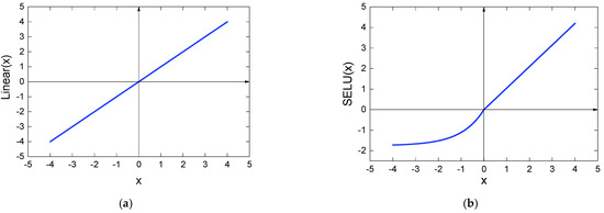
Figure 1.
Linear and SELU activation functions: (a) Linear activation functions; (b) SELU activation functions.
3.3. Architecture and Parameters of the Proposed Method
The architecture of the proposed method is illustrated in Figure 2, which is established in three steps:
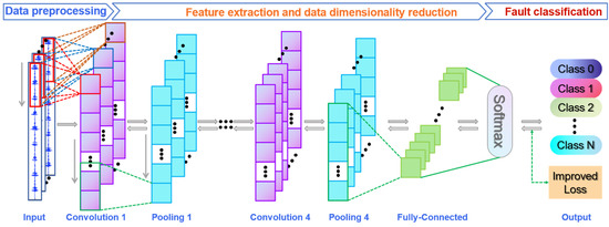
Figure 2.
Architecture of the proposed 1DCNN-L2SVM.
- (1)
- Data preprocessing: the time-sequential signal is intercepted according to the sample length, and the samples of is constructed after preprocessing; is the number of samples.
- (2)
- Feature extraction and data dimensionality reduction: four alternating convolution and pooling layers are established layer by layer. Through multi-layer feature extraction, the more abstract and deeper signal features hidden in the data can be obtained. Through multi-layer pooling operation, the high-dimensional data can be transformed into low-dimensional data for subsequent data classification. Moreover, after the convolution layer, batch normalization is introduced to adjust the data distribution so as to accelerate the convergence process as well as improve the generalization ability of the model. The ReLU in traditional CNN is improved to Linear and SELU to avoid a large amount of data being suppressed before feature extraction, which will affect its recognition accuracy.
- (3)
- Fault classification: the cross-entropy loss is replaced by the L2-SVM loss, and two new parameters, namely, the dynamic adjustment parameter and the modulation factor, are introduced to increase the recognition accuracy of the minority class samples.
The main model parameters that need to be designed are the size and number of convolution kernels (pooling kernels). As to the size of the convolution kernel, the first layer adopts 16 × 1 for the purpose of better suppression of the input of high-frequency noise [39]. The following convolution layers are 3 × 1, which is convenient for network deepening; this improves the feature learning ability of the model. After each convolutional layer, a 2 × 1 maximum pooling operation is performed to lessen the number of network parameters, decrease the time of convolutional operations, and effectively avoid overfitting. In addition, a padding operation is added to each convolutional layer in order not to discard the feature information of the input samples and to keep the output dimension of the convolutional layer consistent with the input dimension.
The effect of model training is also affected by the training parameters. A too-small batch size will cause serious vibration to the loss, and the convergence within the maximum iteration may be difficult; meanwhile, the opposite situation could affect the generalization capability of the model. The batch size is finally set to 128, and the maximum iteration number is 20. The specific parameters of the model are listed in Table 1.

Table 1.
Parameters of the proposed 1DCNN-L2SVM.
3.4. Fault Diagnosis Process
The designed model (Figure 2) is applied to a rotating machinery fault diagnosis system; its application procedure is illustrated in Figure 3, and the implementation steps are outlined below:
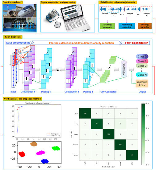
Figure 3.
Flow chart of the fault diagnosis method based on 1DCNN and L2-SVM.
Step 1: The vibration signal of rotating machinery is acquired by the data collection system.
Step 2: The vibration signal is normalized, and each sample is obtained by the sliding window method within 1024 data points. The samples are separated into three parts for training, validating, and testing.
Step 3: The CNN model is built, the ReLU activation function in the traditional CNN is replaced with Linear and SELU activation functions, and the cross-entropy loss is replaced by the L2-SVM loss. Simultaneously, two new parameters are introduced, namely, the dynamic adjustment parameter and the modulation factors. Then, initialize the parameters in the model.
Step 4: The samples for training and validating samples are imported to the model for iterative training. The output label of each sample is predicted, and its estimation error compared to the real one is calculated using the improved L2-SVM loss.
Step 5: Judge whether the model converges. If it converges, jump to step 7; otherwise, turn to step 6.
Step 6: Back propagate the error value obtained in step 4 to each node layer by layer; then, update the weights and biases and repeat steps 4 to 5 until the network converges.
Step 7: The testing samples are imported to the trained model to verify the effectiveness of the proposed method.
4. Experimental Verification
To testify the validity of the proposed method, this section uses Case Western Reserve University (CWRU) bearing datasets [40] and the lab-measured bearing datasets for the experiments, respectively. The software environment is: Python3.7, Tensorflow2.3, and keras2.7. The hardware environment is: Intel i7-4800h + NVIDIA 2060. In this work, Python, Origin, and CorelDraw are mainly used to draw and output the images.
4.1. Case Study 1: Application in CWRU Datasets
4.1.1. Experimental Setup
The bearing datasets of CWRU have high data quality and obvious fault characteristics, so it is a commonly used standard bearing fault diagnosis dataset. In this section, three unbalanced datasets under different loads are constructed to testify to the recognition effect of the proposed method. In Figure 4, the test bench is composed of a 2HP (1.5KW) induction motor, a fan-end bearing, a driver-end bearing, a torque translator, and a load motor. By using EDM technology, single point faults with different depths were machined on the inner race, outer race, and rolling element of the test bearing. The fault diameters were 7, 14, and 21 mils, respectively.
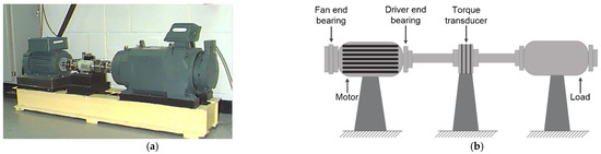
Figure 4.
The motor-bearing test bench of CWRU: (a) real-life diagram of test rig; (b) structure schematic diagram of test rig.
The vibration signals of the drive end bearing, collected under three loads of 0, 1, and 2 HP, are represented by A, B, and C, respectively, as shown in Table 2. In each load, it contains a normal signal, a rolling element fault signal, an inner ring raceway fault signal, and an outer ring raceway fault signal. Among them, the fault signal includes three states with fault diameters of 7, 14, and 21 mils, respectively. Therefore, each load constitutes 10 different data samples, and its time-domain diagram is shown in Figure 5.
Table 2.
Bearing datasets.
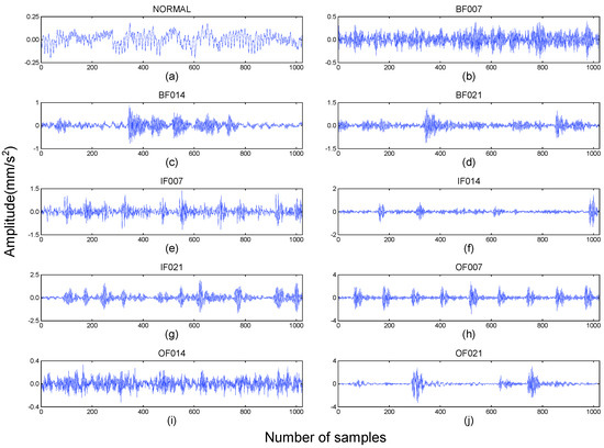
Figure 5.
Vibration signals of bearing: (a) normal; (b) ball fault (007); (c) ball fault (014); (d) ball fault (021); (e) inner fault (007); (f) inner fault (014); (g) inner fault (021); (h) outer fault (007); (i) outer fault (014); (j) outer fault (021).
In the actual working environment, normal signals are often the vast majority of signals, while faults occur occasionally. In order to simulate this actual situation, three datasets were constructed, as listed in Table 2. In Dataset A, the number and proportion of samples for each health condition are the same, so Dataset A is a balanced dataset. In Dataset B, 3000 samples are collected for normal signals (1024 data points for each sample), 300 are collected for rolling element fault signals, 400 for inner race fault signals, and 500 for outer race fault signals. It is clear that the number of samples of normal signals is much larger than the other samples, and the proportion of sets on training, validation, and testing is also different in each state of the signal, thus constituting an unbalanced dataset. In Dataset C, the number of normal signals increases to 10,000, while the number of signals in other health conditions is reduced compared with Dataset B. Therefore, Dataset C is considered to be a highly unbalanced dataset.
4.1.2. Diagnostic Results and Analysis
The three datasets in Table 2 are applied to verify the model, and the results are illustrated in Figure 6. For each block in the matrix square, the horizontal side means the predicted category label and the vertical side means the actual category label; the values of the dark-colored left diagonal line are the number of samples correctly predicted by the model for each sample. It is clear that a larger value reflects the superior classification of the model. In Dataset A, all samples were identified correctly. In Dataset B, three samples in BF014 were identified incorrectly. In Dataset C, a total of 12 samples of BF007 and BF021 were identified incorrectly. In summary, the overall identification accuracy of the model on the two unbalanced datasets is 99.25%, of which the average identification accuracy for the minority class samples is 99.16%. From the experimental results, we can conclude that the improved model obtains more excellent accuracy for the minority class samples in the unbalanced fault diagnosis of CWRU-bearing datasets.
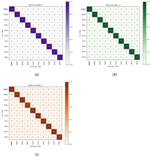
Figure 6.
Confusion matrix of different datasets: (a) the result of Dataset A; (b) the result of Dataset B; (c) the result of Dataset C.
4.1.3. Feature Learning Capability
To visually analyze the feature learning effect of the proposed method on the unbalanced datasets, the test samples in Dataset C were input to the model and the middle layer features learned by the model were extracted. Then, the features were reduced from high-dimension to two-dimension and visualized using t-SNE. The outcomes are represented in Figure 7, in which the middle part is the model’s network composition. Different colors in Figure 7a–f represent different samples, and each point represents one sample. It can be seen from Figure 7a that due to the influence of noise, redundancy, and other factors, all samples are mixed together. After the input signals are extracted by the first convolutional pooling layer, the sample distribution of each category is improved, but it is still difficult to distinguish, as shown in Figure 7b. After the second convolutional pooling layer feature extraction, the samples of 5 states, such as OF021, NORMAL, IF014, IF007, and IF021, are more obviously aggregated, but the other five categories are still difficult to distinguish, as shown in Figure 7c. After further feature extraction by the third convolutional pooling layer, the four classes of samples, such as BF021, IF007, IF021, and OF021, are basically separated, and NORMAL, BF014 and IF014 gather obviously; however, the other three categories are still mixed together, as shown in Figure 7d. After the fourth convolutional pooling layer feature extraction, most samples have been completely separated, and only two classes of samples, BF007 and OF007, are still not completely aggregated, as shown in Figure 7e. At the end of the model, two full connection layers are designed, of which the second one is used for classification, so only the feature extraction of the first one is visualized, as in Figure 7f. It indicates that all the samples of 10 different categories have been separated, and the samples of the same category are completely clustered in the same area.
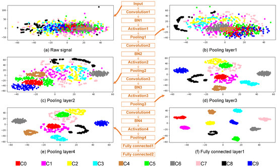
Figure 7.
Visualization of features learned in different layers.
From the above analysis, the original vibration signal can clearly output the signal features hidden in the data to the new space after convolution and pooling. In the process of feature extraction layer by layer, the information learned in the shallow layer is usually simple signal features. Until now, those samples are still difficult to distinguish, and with the increase in the number of network layers, the model can abstract higher dimensional fault features, and various input samples can be well identified according to these features.
4.1.4. Comparison Experiments
In this section, the goal of experimental verification of the proposed method is the more effective identification of unbalanced datasets. Six fault identification algorithms are used for comparison experiments. (1) Compared with BPNN and SVM, which require manual feature extraction. The data in Table 2 are first extracted with 10 time-domain features shown in Table 3 and Table 4 frequency-domain features shown in Table 5, and then the extracted 15 feature samples are input to BPNN and SVM for fault identification. Among them, the kernel function of SVM uses a Gaussian radial basis function (RBF) with C = 10; the hidden layer structure of BPNN is (32,16), and the activation function is ReLU. (2) the CNN using the ReLU function (R-CNN) and the CNN using the SELU function (S-CNN) are used for classification. (3) Compared with commonly used unbalanced data fault identification methods, CNN (CSCNN) and SMOTE-CNN are more cost-sensitive. The network structure and parameters of CSCNN are consistent with the proposed method, and the cost matrix is determined by the sample proportion. After SMOTE sampling, unbalanced training samples become balanced samples, and then fault identification is carried out through CNN. The data in Table 3 are used to conduct experiments. Note that each experiment is conducted 20 times to eliminate the impact of stochastic values. The experimental results are shown in Figure 8. We use accuracy as the evaluation metric, which is a commonly used index to measure the performance of classification problems. Its formula is
where (true positive) is correctly classified as a positive sample, (true negative) is correctly classified as a negative sample, and is the total number of samples.
Table 3.
Features selected in the time domain.
Table 4.
Features selected in the frequency domain.
Table 5.
Bearing dataset descriptions.
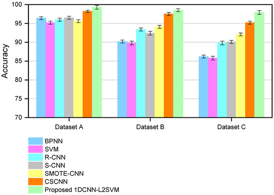
Figure 8.
Identification accuracies on three datasets by seven methods.
Since Dataset A is a balanced dataset, all seven methods obtained high accuracy. In the unbalanced Dataset B, the minority class samples used to train these methods become fewer in number; therefore, the accuracy of all seven methods decreased. Among them, the accuracy of BPNN and SVM decreased to 90.2% and 89.8%, respectively. This is because BPNN and SVM need manual feature extraction before training. However, the manually extracted features are not comprehensive and the key features may be missed, resulting in a rapid decline in accuracy. In addition, the accuracy of R-CNN is 93.4%, S-CNN is 92.4%, SMOTE-CNN is 94.1%, CSCNN is 97.5%, and 1DCNN-L2SVM is 98.5%. Obviously, 1DCNN-L2SVM obtains the highest accuracy because it uses dynamic adjustment parameters and modulation factors to deal with unbalanced data. The samples in Dataset C are more unbalanced than those in dataset B. The accuracy of BPNN decreases from 90.2% to 86.2%, while SVM decreases from 89.8% to 85.8%, R-CNN from 93.4% to 89.8%, S-CNN from 92.4% to 90.1%, SMOTE-CNN from 94.1% to 92.1%, and CSCNN from 97.5% to 95.2%. In contrast, the accuracy of 1DCNN-L2SVM is 97.9%, which is only a 0.6% decrease. Therefore, the proposed 1DCNN-L2SVM outperforms several other methods in unbalanced fault classification.
4.2. Case Study 2: Application to the Lab-Measured Bearing Datasets
4.2.1. Experimental Setup
As in Section 4.1, the presented 1DCNN-L2SVM has achieved high identification accuracy for the minority class samples on the CWRU-bearing datasets, but the validity of the model in reality still needs to be further studied. Therefore, in this section, we use a comprehensive experimental bench from Wuxi Houde Automation Meter Co., Ltd. (Wuxi, China) to collect unbalanced datasets at four different rotational speeds for experiments. As shown in Figure 9, the experimental bench is composed of a motor, coupling, a mass block, a shaft, an acceleration sensor, an experiment bearing (NSK6308), an eddy current sensor, and other devices. Among them, the shaft is a cylindrical object passing through the middle of a bearing. It supports rotating parts and rotates with them to transmit motion, torque, or bending moment. The acceleration sensor is usually composed of a mass block, a damper, an elastic element, a sensing element, and an adaptive circuit. It is mainly used to measure the vibration signal of bearings. In the experiment, the normal bearing and four kinds of fault bearings were installed on the experiment bench successively, and the acceleration sensor (HD-YD232) was the collection component of the bearing vibration signals in different states. Its sampling frequency is 8 kHz.
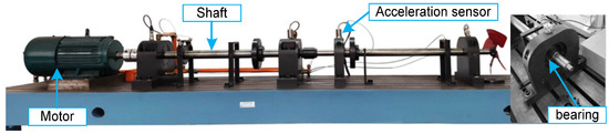
Figure 9.
Accelerated bearing life tester.
The vibration signals of the bearings are collected at three different speeds of 2600, 2800, and 3000 r/min and represented by A, B, and C, as listed in Table 5. At one speed, five different data samples are collected, which include: (1) a rolling element fault signal, (2) a cage fault signal, (3) an inner ring raceway fault signal, (4) a normal signal, and (5) an outer ring raceway fault signal. Figure 10 describes the time and frequency domain diagrams of those signals.
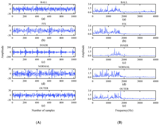
Figure 10.
Time domain and frequency domain diagram of test bearing: (A) time-domain waveform; (B) frequency-domain waveform.
In Table 5, compared with the balanced Dataset A, the number of minority class samples is reduced in the unbalanced Dataset B. Moreover, the proportions of the training, validation, and testing sets are different among each sample. In Dataset C, the number of normal samples increases substantially to 8000, so Dataset C is a highly unbalanced dataset.
4.2.2. Diagnostic Results and Analysis
Figure 11 shows the verification results of the three datasets in Table 5, operated by the improved model. In Dataset A, all samples are identified correctly. In Dataset B, two samples of FIX are incorrectly identified as NORMAL. In Dataset C, six samples of FIX are incorrectly identified as NORMAL. It can be seen that in the two unbalanced datasets, the model mistakenly identifies some FIX samples as NORMAL. Due to the minimum number of FIX training samples, the feature learning is insufficient. At the same time, since NORMAL is the majority class, the features extracted by the model during the training process are more biased toward NORMAL, which coincides with the idea that the model may give rise to more bias in features learned toward the majority class samples when the data are unbalanced, as we predicted in the previous section. Despite these difficulties, the proposed method overcomes this difficulty well and achieves an overall discrimination accuracy of 99.2% on the two unbalanced datasets, with an average discrimination accuracy of 99.0% for the minority class samples. The results further confirm that the modified method obtains better precision for the minority class samples in the lab-measured bearing datasets and has a certain generalization performance.
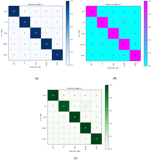
Figure 11.
The confusion matrix of different datasets: (a) the result of Dataset A; (b) the result of Dataset B; (c) the result of Dataset C.
4.2.3. Feature Learning Capability
To visually analyze the feature learning effect of the proposed method on the unbalanced datasets, the test samples in Dataset C are input to the model and the middle layer features learned by the model are extracted. Then, the features are reduced from high-dimension to two-dimension and visualized using t-SNE. The results are shown in Figure 12, in which the middle part is the network structure of the model. Different colors in Figure 12a–f represent different samples, and each point represents one sample. It can be seen from Figure 12a that due to the influence of noise, redundancy, and other factors, various samples are mixed together. After the input signals are extracted by the first and second convolution pooling layers, the sample distribution of each category is improved, but it is still difficult to distinguish, as shown in Figure 12b,c. After further feature extraction of the third convolution pooling layer, the normal samples (blue) and the outer ring raceway fault samples (red) are obviously gathered, as shown in Figure 12d. After the fourth convolutional pooling layer feature extraction, the normal samples (blue) and the outer race raceway fault samples (red) are completely separated, and the other three types of samples are gathered, as shown in Figure 12e. After the fully connected layer, the samples of the five different categories are all separated, and the samples of the same category are completely gathered in the same area, as shown in Figure 12f. We can also see that the normal samples (blue) are separated first because they contain the largest number of samples (10,000 samples). The second sample separated is the outer ring fault samples (red), which contain the second largest number of samples (500 samples).
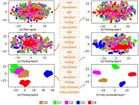
Figure 12.
Visualization of features learned in different layers.
From the above analysis, the number of samples has a great impact on model training. When the data are unbalanced, the recognition accuracy of the minority class samples is easily affected by the smaller number of samples. The results further show that the proposed method overcomes this shortcoming, obtains high accuracy, and can learn the essential data features hidden in the raw vibration signals.
5. Conclusions
In this paper, we propose a new fault diagnosis method for unbalanced data based on improved 1DCNN and L2-SVM. Firstly, the ReLU activation function in the traditional CNN is replaced with Linear and SELU activation functions. Linear is used in the input layer to ensure that all minority class samples can enter the model for training to improve its recognition accuracy. SELU is used in the middle layer to overcome the disadvantage that ReLU is more fragile during the training process. Secondly, the four convolution pooling layers are used to extract the more abstract and deeper signal features implied in the input data, layer by layer, and then the extracted signal features are mapped to the class space through the full connection layer. In the class space, the cross-entropy loss is replaced by the L2-SVM loss, and a dynamic adjustment parameter is introduced to assign a lower misclassification cost to the majority class samples and more cost to the minority class samples. Finally, we add another modulation factor to reduce the weight of easy-to-classify samples and let the model focus on training a small number of hard-to-classify samples during the training process.
Three datasets with different unbalanced degrees under different loads are constructed based on the CWRU public bearing dataset, and similar datasets under different speeds are constructed based on the lab-measured bearing dataset. All these datasets are used to check the validity of the presented method. The experiments prove that our method has higher recognition accuracy when dealing with unbalanced datasets. Then, further comparison experiments were carried out with six other commonly used methods. The results show that the proposed method has obvious advantages over traditional machine learning methods such as BPNN and SVM. The reason is that the proposed method does not need any manual feature extraction and selection process, and the extracted features have more comprehensive and deeper characteristics.
Compared with R-CNN and S-CNN, which use the traditional single activation function, the proposed method also obtains certain advantages, which proves the effectiveness of the improvement of the activation function in this paper. Even compared with the commonly used unbalanced data fault identification methods, cost-sensitive CNN (CSCNN) and SMOTE-CNN, it still has certain advantages because this research designs two new parameters, namely, dynamic adjustment parameters and modulation factors. Dynamic adjustment parameters make the model improve the weight of the majority class samples during training, while modulation factors reduce the weight of more distinguishable samples. Under the joint action of the two designed parameters, the diagnostic accuracy of the indiscernible samples has been increased.
In the future, transfer learning and multi-scale will be introduced to elevate the domain adaptability of the model. In addition, there are some possible misclassifications, so it is necessary to apply the proposed model to more environments, considering other datasets and integration methods to further optimize the model.
Author Contributions
Methodology, B.H. and J.L.; software, B.H. and T.H.; writing—original draft preparation, B.H.; writing—review and editing, J.L. and R.Z.; supervision, Y.X.; data curation, T.H. All authors have read and agreed to the published version of the manuscript.
Funding
This research was funded by the National Natural Science Foundation of China (71861025 and 51675253), the National Key Research and Development Plan (Grant Number 2018YFB1703105), and the Hongliu First-class Disciplines Development Program of Lanzhou University of Technology.
Institutional Review Board Statement
Not applicable.
Informed Consent Statement
Not applicable.
Data Availability Statement
The data presented in this study are available upon request from the corresponding author.
Conflicts of Interest
The authors declare no conflict of interest.
References
- Wang, Q.; Zhao, B.; Ma, H.; Chang, J.; Mao, G. A method for rapidly evaluating reliability and predicting remaining useful life using two-dimensional convolutional neural network with signal conversion. J. Mech. Sci. Technol. 2019, 33, 2561–2571. [Google Scholar] [CrossRef]
- Rai, A.; Upadhyay, S.H. A review on signal processing techniques utilized in the fault diagnosis of rolling element bearings. Tribol. Int. 2016, 96, 289–306. [Google Scholar] [CrossRef]
- Widodo, A.; Yang, B.-S. Support vector machine in machine condition monitoring and fault diagnosis. Mech. Syst. Signal Process. 2007, 21, 2560–2574. [Google Scholar] [CrossRef]
- Lei, Y.; Lin, J.; He, Z.; Zuo, M.J. A review on empirical mode decomposition in fault diagnosis of rotating machinery. Mech. Syst. Signal Process. 2013, 35, 108–126. [Google Scholar] [CrossRef]
- Feng, Z.; Liang, M.; Chu, F. Recent advances in time-frequency analysis methods for machinery fault diagnosis: A review with application examples. Mech. Syst. Signal Process. 2013, 38, 165–205. [Google Scholar] [CrossRef]
- Li, C.; de Oliveira, J.V.; Cerrada, M.; Cabrera, D.; Sánchez, R.V.; Zurita, G. A Systematic Review of Fuzzy Formalisms for Bearing Fault Diagnosis. IEEE Trans. Fuzzy Syst. 2019, 27, 1362–1382. [Google Scholar] [CrossRef]
- Xu, G.; Liu, M.; Jiang, Z.; Söffker, D.; Shen, W. Bearing Fault Diagnosis Method Based on Deep Convolutional Neural Network and Random Forest Ensemble Learning. Sensors 2019, 19, 1088. [Google Scholar] [CrossRef] [PubMed]
- Landauskas, M.; Cao, M.; Ragulskis, M. Permutation entropy-based 2D feature extraction for bearing fault diagnosis. Nonlinear Dyn. 2020, 102, 1717–1731. [Google Scholar]
- Hinton, G.E.; Salakhutdinov, R.R. Reducing the Dimensionality of Data with Neural Networks. Science 2006, 313, 504–507. [Google Scholar] [PubMed]
- LeCun, Y.; Bengio, Y.; Hinton, G. Deep learning. Nature 2015, 521, 436–444. [Google Scholar] [CrossRef] [PubMed]
- Mousavi, N.S.; Vaferi, B.; Romero-Martínez, A. Prediction of Surface Tension of Various Aqueous Amine Solutions Using the UNIFAC Model and Artificial Neural Networks. Ind. Eng. Chem. Res. 2021, 60, 10354–10364. [Google Scholar] [CrossRef]
- Zhou, Z.; Davoudi, E.; Vaferi, B. Monitoring the effect of surface functionalization on the CO2 capture by graphene oxide/methyl diethanolamine nanofluids. J. Environ. Chem. Eng. 2021, 9, 106202. [Google Scholar]
- Otter, D.W.; Medina, J.R.; Kalita, J.K. A Survey of the Usages of Deep Learning for Natural Language Processing. IEEE Trans. Neural Netw. Learn. Syst. 2021, 32, 604–624. [Google Scholar] [CrossRef] [PubMed]
- Kuang, F.; Zhou, X.; Liu, Z.; Huang, J.; Liu, X.; Qian, K.; Gryllias, K. Computer-vision-based research on friction vibration and coupling of frictional and torsional vibrations in water-lubricated bearing-shaft system. Tribol. Int. 2020, 150, 106336. [Google Scholar] [CrossRef]
- Jiao, L.; Zhao, J. A Survey on the New Generation of Deep Learning in Image Processing. IEEE Access 2019, 7, 172231–172263. [Google Scholar] [CrossRef]
- Roshani, M.; Sattari, M.A.; Muhammad Ali, P.J.; Roshani, G.H.; Nazemi, B.; Corniani, E.; Nazemi, E. Application of GMDH neural network technique to improve measuring precision of a simplified photon attenuation based two-phase flowmeter. Flow Meas. Instrum. 2020, 75, 101804. [Google Scholar] [CrossRef]
- Khalil, R.A.; Jones, E.; Babar, M.I.; Jan, T.; Zafar, M.H.; Alhussain, T. Speech Emotion Recognition Using Deep Learning Techniques: A Review. IEEE Access 2019, 7, 117327–117345. [Google Scholar] [CrossRef]
- Vaferi, B.; Eslamloueyan, R. Hydrocarbon reservoirs characterization by co-interpretation of pressure and flow rate data of the multi-rate well testing. J. Pet. Sci. Eng. 2015, 135, 59–72. [Google Scholar] [CrossRef]
- Aljemely, A.H.; Xuan, J.; Jawad, F.K.J.; Al-Azzawi, O.; Alhumaima, A.S. A novel unsupervised learning method for intelligent fault diagnosis of rolling element bearings based on deep functional auto-encoder. J. Mech. Sci. Technol. 2020, 34, 4367–4381. [Google Scholar] [CrossRef]
- Zhou, K.; Cao, G.; Zhang, K.; Liu, J. Domain adaptation-based deep feature learning method with a mixture of distance measures for bearing fault diagnosis. Meas. Sci. Technol. 2021, 32, 095105. [Google Scholar] [CrossRef]
- Pan, T.; Chen, J.; Qu, C.; Zhou, Z. A method for mechanical fault recognition with unseen classes via unsupervised convolutional adversarial auto-encoder. Meas. Sci. Technol. 2021, 32, 035113. [Google Scholar] [CrossRef]
- Nguyen, V.H.; Cheng, J.S.; Yu, Y.; Thai, V.T. An architecture of deep learning network based on ensemble empirical mode decomposition in precise identification of bearing vibration signal. J. Mech. Sci. Technol. 2019, 33, 41–50. [Google Scholar] [CrossRef]
- Shao, H.; Jiang, H.; Wang, F.; Zhao, H. An enhancement deep feature fusion method for rotating machinery fault diagnosis. Knowl. Based Syst. 2017, 119, 200–220. [Google Scholar] [CrossRef]
- Jing, L.; Zhao, M.; Li, P.; Xu, X. A convolutional neural network based feature learning and fault diagnosis method for the condition monitoring of gearbox. Measurement 2017, 111, 1–10. [Google Scholar] [CrossRef]
- Wen, L.; Li, X.; Gao, L.; Zhang, Y. A New Convolutional Neural Network-Based Data-Driven Fault Diagnosis Method. IEEE Trans. Ind. Electron. 2018, 65, 5990–5998. [Google Scholar] [CrossRef]
- Mukhopadhyay, R.; Panigrahy, P.S.; Misra, G.; Chattopadhyay, P. Quasi 1D CNN-based Fault Diagnosis of Induction Motor Drives. In Proceedings of the 2018 5th International Conference on Electric Power and Energy Conversion Systems (EPECS), Kitakyushu, Japan, 23–25 April 2018; IEEE: Piscataway, NJ, USA, 2018; pp. 1–5. [Google Scholar]
- Chen, R.; Huang, X.; Yang, L.; Xu, X.; Zhang, X.; Zhang, Y. Intelligent fault diagnosis method of planetary gearboxes based on convolution neural network and discrete wavelet transform. Comput. Ind. 2019, 106, 48–59. [Google Scholar] [CrossRef]
- Hoang, D.-T.; Kang, H.-J. Rolling element bearing fault diagnosis using convolutional neural network and vibration image. Cogn. Syst. Res. 2019, 53, 42–50. [Google Scholar] [CrossRef]
- Lessmeier, C.; Kimotho, J.; Zimmer, D.; Sextro, W. Condition Monitoring of Bearing Damage in Electromechanical Drive Systems by Using Motor Current Signals of Electric Motors: A Benchmark Data Set for Data-Driven Classification. In Proceedings of the European Conference of the PHM Society 2016, Bilbao, Spain, 5–8 July 2016. [Google Scholar]
- Ince, T.; Kiranyaz, S.; Eren, L.; Askar, M.; Gabbouj, M. Real-Time Motor Fault Detection by 1-D Convolutional Neural Networks. IEEE Trans. Ind. Electron. 2016, 63, 7067–7075. [Google Scholar] [CrossRef]
- Eren, L. Bearing Fault Detection by One-Dimensional Convolutional Neural Networks. Math. Probl. Eng. 2017, 2017, 8617315. [Google Scholar] [CrossRef]
- Huang, S.; Tang, J.; Dai, J.; Askar, M.; Gabbouj, M. Signal Status Recognition Based on 1DCNN and Its Feature Extraction Mechanism Analysis. Sensors 2019, 19, 2018. [Google Scholar] [CrossRef]
- Li, H.; Huang, J.; Ji, S. Bearing Fault Diagnosis with a Feature Fusion Method Based on an Ensemble Convolutional Neural Network and Deep Neural Network. Sensors 2019, 19, 2034. [Google Scholar] [CrossRef]
- Cao, J.; He, Z.; Wang, J.; Yu, P. An Antinoise Fault Diagnosis Method Based on Multiscale 1DCNN. Shock Vib. 2020, 2020, 8819313. [Google Scholar] [CrossRef]
- Liu, Z.; Wang, H.; Liu, J.; Qin, Y.; Peng, D. Multitask Learning Based on Lightweight 1DCNN for Fault Diagnosis of Wheelset Bearings. IEEE Trans. Instrum. Meas. 2021, 70, 1–11. [Google Scholar] [CrossRef]
- Huang, S.; Tang, J.; Dai, J.; Wang, Y. 1DCNN Fault Diagnosis Based on Cubic Spline Interpolation Pooling. Shock Vib. 2020, 2020, 1949863. [Google Scholar] [CrossRef]
- Jia, F.; Lei, Y.; Lu, N.; Xing, S. Deep normalized convolutional neural network for imbalanced fault classification of machinery and its understanding via visualization. Mech. Syst. Signal Process. 2018, 110, 349–367. [Google Scholar] [CrossRef]
- Tang, Y. Deep Learning using Linear Support Vector Machines. arXiv 2015, arXiv:1306.0239. [Google Scholar]
- Zhang, W.; Peng, G.; Li, C.; Chen, Y.; Zhang, Z. A New Deep Learning Model for Fault Diagnosis with Good Anti-Noise and Domain Adaptation Ability on Raw Vibration Signals. Sensors 2017, 17, 425. [Google Scholar] [CrossRef]
- CWRU. Case Western Reserve University Bearing Date Center Website; CWRU: Cleveland, OH, USA, 2006; Available online: https://engineering.case.edu/bearingdatacenter/download-data-file (accessed on 12 January 2020).


Publisher’s Note: MDPI stays neutral with regard to jurisdictional claims in published maps and institutional affiliations. |
© 2022 by the authors. Licensee MDPI, Basel, Switzerland. This article is an open access article distributed under the terms and conditions of the Creative Commons Attribution (CC BY) license (https://creativecommons.org/licenses/by/4.0/).