Abstract
In this study, a mixed integer, linear, multi-stage, stochastic programming model is developed for multi-product aggregate production planning (APP). An approximation is used with a model that employs discrete distributions with three and four values and their respective probabilities of occurrence for the random variables, which are demand and production capacity, each one for every product family. The model was solved using the deterministic equivalent of the multi-stage problem using the optimization software LINGO 19.0. The main objective of this research is to determine a feasible solution to a real APP in a reasonable computational time by comparing different methods. Since the deterministic equivalent was difficult to solve, a proposal model with bounds in some decision variables was developed using some properties of the original model; both models were solved for different periods. We demonstrated that the proposed model had the same solution as the original model but required fewer iterations and CPU time, which implies an advantage in real APP. Finally, a sensitivity analysis was performed at varying service levels finding that if the service levels increase, the cost increases as well.
1. Introduction
The Aggregate Production Plan (APP) aims to meet customer requirements at the lowest investment and operation cost [1], considering production, inventory and workforce in a planning horizon [2]. In a highly competitive environment for companies, it is necessary to find effective solutions in the shortest possible time [3], increasing customer service [4] and managing uncertainty in different variables [5].
Considering the uncertainty in demand and service levels makes the problem highly complex [6]; also, real-world problems are multi-product and multi-period [7], causing insufficiency of traditional methods [3,8]. For this reason, additional methods to deterministic and stochastic optimization have been proposed to deal with the complexity, adding to the literature methods, such as extended for order performance [2], hierarchical production planning [4], fuzzy logic [5], hybrid algorithm based in simulated annealing (SA) and simplex downhill (SD) [9] particle swarm optimization algorithm (PSO) which considered labor characteristics, modeled as integer linear programming [10], among others.
The multi-product APP is the model that considers more than one family product [11], minimizing total production costs and improving efficiency of equipment. Mehdizadeh, Niaki and Hemati [12] proposed a multi-product APP as a bi-objective problem, the first objective maximizing the profit through the improvement of the learning curve in workers and the second objective minimizing the repairs and deterioration of the machines. APP includes families of products or products that have the same production processes [13]. Darvishi et al. [7] consider multi-site APP problems in multi-period, multi-product and multiple transportation modes under uncertainty, which means, restrictions that deal with real situations.
Additionally, it has been necessary to adapt the problem to specific cases, such as the agrifood supply chain [5], power systems [1], pharmaceutical industry [14] and apparel production [7], because it is related to its objectives and specific characteristics. There is no single production plan; each company works its APP differently according to the purposes of its organization.
The formulation of an APP through mathematical programming seeks to minimize costs or maximize profits. One of the most important aspects to consider is the types of variables. The variables included in the model are important because they allow the APP to be adequate or not for an enterprise. Similarly, they impact the costs (the value of the objective function). Most of the variables used are demand, number of workers, production capacity, quantity to be produced and inventory, as is usual in the literature [1,2].
Some models may include more or fewer variables, depending on the needs of the organization; in the same way, they may have one or more objectives, as well as various types of constraints [11,12]. Ideally, an APP should be aligned with the production and contracting capabilities of the organization, forecasted demand (if it is forecasted), inventory levels, availability of raw materials, resources for processing and external factors that may affect the organization such as the local economy or competitors.
APP is used in medium-term horizons with periods from 3 to a maximum of 18 months [15]. Similarly, it is usual that one or more of the parameters in the APP are considered random (the most used in the literature is demand), but not limited to the percentage of defective products (product quality), production costs, machine failure, quality of inputs, among others, allowing planning to be more realistic.
The motivation of this work was extending a real developed project of Gómez-Rocha et al. [16] in a furniture manufacturer, improving productivity with optimal policies for production, inventory and backlogs, while minimizing production costs, considering the existence of stochastic parameters in the APP and now, with a multi-product approach, without a hiring–firing policy because some researchers found that this has a negative impact in the capacity production and, in some cases, implies trouble with syndicates if the company has one [17,18], such as the enterprise under this study. Although there are different approaches to deal with the APP complexity, for this research, a stochastic programming model is proposed with valid inequalities; to our knowledge, this approach has not been considered before in the literature.
The paper is organized as follows: in Section 2, the literature review is presented considering different approaches to solve APP with stochastic demand and presenting the novelty of this work. In Section 3, the models are presented: deterministic, multi-stage stochastic programming model and method to generate upper and lower bounds (valid inequalities) in some decision variables in the last model. In Section 4, the results are explained in a case for the industry with two family products. Finally, the conclusions are presented in Section 5.
2. Literature Review
2.1. APP under Uncertainty
APP under uncertainty can be modeled and studied using fuzzy models, stochastic models, simulation, metaheuristics or evidential reasoning and can be single-objective or multi-objective, as mentioned by Cheraghalikhani, Khoshalhan and Mokhtari [11] and Jamalnia et al. [15]. The behavior of the randomness determines the proper model to use. When the uncertainty can be represented as a probability distribution known (continuous or discrete), stochastic programming works better; in other cases, where human criteria and decisions become important in terms of linguistic variables, fuzzy models are the best option [5].
Jamalnia and Feili [19] present simulation models comparing different strategies in APP, such as pure chase strategy, pure level strategy among others, and Li et al. [20] use evidential reasoning for solving APP with uncertain demand.
Some studies about APP solved using fuzzy models were performed by Gholamian et al. [21]. They proposed a new fuzzy programming method in a multi-objective mixed integer nonlinear programming model, and Gholamian et al. [22] extend the previous work considering conflictual objectives.
Besides that, metaheuristics were used in APP, although when stochastic parameters are used the method performance is not the best option since the deterministic equivalent is complex to solve when the number of the scenarios and stages increases; however, Aliev et al. [23] show a study using a hybrid fuzzy–genetic approach.
Since this work uses stochastic programming, the next part of the literature review is focused on this solution approach considering the model class, number of objectives and the methods to solve it, and these features are explained in the next paragraphs.
2.2. Stochastic Programming for Solving APP
Jamalnia et al. [24] mentioned that many of the APP are nonlinear and multi-objective. They present a model with these characteristics with demand as a source of uncertainty and a discrete empirical distribution of probability. In their study, only the Wait-and-See (WS) solution of each objective function is reported, they dropped the non anti-cipativity constraints because the model was difficult to solve, they used the Pareto optimal and the problem was solved using www-NIMBUS [25].
Zhao et al. [26] presented a model with two objectives, formulated using multi-stage stochastic programming, where the source of uncertainty was hiring patients for trial clinics with a Poisson probability distribution. In their model, they used the Progressive Hedging Algorithm (PHA) and the Sample Average Approximation (SAA), they reported the time to solve the problem, the memory used among others, only the RP (Here-and-Now) solution of each objective function was presented, and they solved the problem using CPLEX.
There have also been developed works where uncertainty exists in production plans with multiple objectives such as Chen and Liao [27]. In general, these classes of models are complex in solution, and if they are not properly formulated, the solutions found are local optima, which may be far from a globally optimal solution.
Single-objective models are the most found in the literature, usually minimizing total production costs, although others may maximize profits (usually after taxes). Kazemi et al. [28] conducted a study using SAA as a solution strategy using a two-stage mixed integer linear programming model solved with CPLEX, and yields were the stochastic parameter.
Later Kazemi et al. [29] focused on the same problem under a stochastic multi-stage problem with an approximate solution using a scenario tree with three possible realizations of random parameters (demand and yields). These points were obtained by a discretization of probability distributions, and later, a scenario decomposition was performed, solved again with CPLEX.
Huang [30], likewise, presented models for production plans using mixed integer linear multi-stage stochastic programming models for the microprocessors industry with random demand. Mirzapour Al-e-hashem et al. [31] developed a methodology to solve a mixed integer nonlinear programming for APP under uncertainty considering some properties of the model, and later made a linearization.
Nasiri et al. [32] proposed a two-stage stochastic mixed integer nonlinear programming model for a supply chain that included production planning as part of the model. They, subsequently, extended their work into a multi-stage model [33]. Nasiri et al. [34] presented a nonlinear model for a three-tier supply chain with a production and distribution plan. Ning et al. [35] presented a multi-product nonlinear model where demand and production cost are uncertain.
Lieckens and Vandaele [36] considered the demand and lead time as random variables. Similarly, Hu and Hu [37] used a scenario tree to solve a sequencing and lot sizing problem with random demand, while Körpeoglu et al. [38] similarly used a scenario tree to solve a master sequencing plan (MPS). In these studies, only the RP or WS solution was reported, and none reported the EVPI. Similarly, few studies performed a sensitivity and those that did, it was only by varying fixed parameters. Neither the level of service nor the impact of varying the parameters of the probability distributions, which are considered in this work, were considered.
When the parameters of the probability distributions are unknown, robust optimization is used to solve the problem. Leung and Wu [39] applied this method by considering economic growth scenarios, minimizing production costs and determining inventory levels, layoffs and hiring. Kanyalkar and Adil [40] considered, in addition to the RP solution for the APP, the WS solution for distribution, i.e., they integrated the APP into the supply chain for a multi-site problem.
Mirzapour Al-e-hashem, Malekly and Aryanezhad [41] also suggested an APP integrated with the supply chain applied to a real case. Considering demand as a source of uncertainty, the model minimized the total production costs associated with production, layoffs, hiring and training of new personnel, as well as minimized the number of backlogs. Mirzapour Al-e-hashem, Aryanezhad and Sadjadi [42] proposed an algorithm for a multi-product, multi-period, multi-site APP using robust optimization. The objective was to minimize production costs and backlogs, as well as maximize worker productivity.
Makui, Heydari, Aazami and Dehghani [43] used accelerated Benders decomposition for problems where products have an extremely limited expiration date, such as can be seen in seasonal clothing or perishable products; demand and production costs are considered as the random variables. As it can be realized from the presented works, few authors recognize in their model a service level constraint [41]; these authors considered minimizing backlog, but without being part of some constraint with some delivery percentage to be fulfilled so then there is a possibility that the service level is not high.
In addition, a limited number of works performed a sensitivity, except for fixed parameters, and none of them consider the variation in the level service or add upper and lower bounds in some decision variables to increase the performance in the CPU time and reduce required iterations using exact methods. That is what is proposed in this research. Table 1 summarizes the most relevant studies in APP under uncertainty solved by stochastic programming and this study.

Table 1.
Comparison of this study with others about APP solved using stochastic programming.
The contribution of this study is the modeling of a real problem where uncertainty affects parameters of the production system; the sources of uncertainty (random variables) are demand and production capacity per period. The family of products are known, and the decision variables are the total workers required, production units, inventory levels and backlogs per period. Upper and lower bounds for first-stage decision variables are calculated using some properties of the model, which implies a more tractable model for solving the APP using stochastic programming. In any study about stochastic programming applied to solve APP, this approach was considered to solve the model.
3. Methods
This section has three subsections. In the first one, we explained the development of a deterministic model (i.e., without consideration of uncertainty) for the APP as a base model and made some assumptions. Then, we developed the multi-stage stochastic programming model and interpreted the new notation and assumptions. Finally, we explained the methodology to obtain the upper and lower bounds for the proposal model. These bounds reduce the number of iterations and CPU time. Next, we present the subsections previously mentioned.
3.1. Deterministic Model for the Aggregate Production Planning
The deterministic model minimizes the total productions cost, determining the number of workers prior to the start of the APP, the number of parts that will be produced and will be stored (inventory) for each period and family of products and the backlogs per month with a specific service level for each period and family of products. The model considers the following assumptions:
- Two families of products are considered.
- The demand and production capacity are known for all periods, i.e., the demand is forecasted and production capacity is estimated for each family of products.
- The fixed costs for parts that are produced, listed in an inventory, backlogs and workers hired, are linear.
- There exists enough raw material to produce all family products over the horizon plan.The notation of the APP is the following:
- Indices: is the set of periods with ; is the set of family products with .
- Parameters: is demand for each period and family product; is production capacity for each period, family product and worker; , and are the inventory, production and backlog costs per unit, family of products and period. is the workers’ cost over the planning horizon, i.e., the total amount to be paid to each worker assigned to each family product for the total/entire APP duration; is the level service for every family product (between 0.8 and 1).
- Decision variables: is the number of workers assigned to production for each product type; , and are the inventory units, parts produced and backlogs per period product.
Equation (1) is the objective function that minimizes total costs production plan. Notice that the cost of the workers assigned to each family products is not for all the periods, which is because without a hiring–firing policy, the workers’ size will be the same for all periods, and then, is the amount to be paid for all the periods in the horizon plan.
Equation (2) is the demand–inventory–backlogs balance; this equation determines the number of parts to be produced, the inventory level and the number of backlogs per period and family of products. Notice that if backlogs occur in some period, then in the following period, the backlogs must be conserved.
Equation (3) is the capacity constraint and indicates that the maximum parts for each period and family of products must be equal or less than the number of workers assigned for each family of products multiplied by the production capacity for each period and family of products.
Equation (4) is the level of service constraint and ensures that a certain percentage of the demand will be completed for each period and family of products.
Constraint (5) indicates nonnegative decision variables for all periods and families of products.
Expression (6) indicates that the backlogs and the inventory must be integer decision variables. Notice that considering only these decision variables as integers, if the demands forecasted are integers, then the decision variable of the number of parts to be produced also will be an integer.
3.2. Multi-Stage Stochastic Programming Model for the Aggregate Production Planning
The multi-stage stochastic programming has the same assumptions as the deterministic model, in addition to the following:
- The methodology used by Gómez-Rocha et al. [16] was considered, obtaining the best fit probability distribution for each stochastic parameter.
- Using best fit distribution test, probability distributions for random variables were found and they are continuous, then, a discretization of distribution probabilities was used and Gaussian quadrature was applied, as explained by Kazemi et al. [30] with three and four possible realizations of random variables.
- First-stage decision variables are the number of workers required for each family of products; after that, in the next stages, the other decision variables are obtained with consideration for the filter process due the stochastic process, in other words, taking into account the nonanticipitave non anticipativity constraints.
- The problem has complete recourse.
Because the APP is now a stochastic programming model, the notation of some decision variables and parameters changes and some sets are added. The notation now is:
- Indices: is the set of periods with ; is the set of family products with ; is the set of all scenarios with ; is the bundle of scenarios that are indistinguishable from in period ; is the random space.
- Parameters: is demand for each period, family product and scenario (stochastic parameter); is production capacity for each period, family product, worker and scenario (stochastic parameter); are the inventory, production and backlog costs per unit, a family of products and period; represents the workers’ cost over the planning horizon, i.e., the total amount to be paid for each worker assigned to each family product for the total duration of the APP; is the level service for every family product; is the probability of occurrence for each scenario with ; is the node in the scenario tree corresponding to each scenario and period; is the probability of .
- Decision variables: is the number of workers assigned to production for each scenario and product type; , , are the inventory units, parts produced and backlogs per period, product type and scenario.
The stochastic programming model for APP is:
Equation (7) is the objective function and seeks to minimize all the production costs across all scenarios, the same as the deterministic model, where is the amount to be paid for all the periods in the horizon plan.
Equation (8) is the demand–inventory–backlogs balance; this equation determines the number of parts to be produced, the inventory level and the number of backlogs, taking into account the uncertainty of each scenario.
Equation (9) is the capacity constraint; as Equation (3) indicates, the maximum number of parts that can be produced for each period, family of products and scenario.
Equation (10) is the level service constraint and ensures that a certain percentage of the demand will be completed for each period, family of products and scenario.
Equations (11)–(14) are the non anticipativity constraints, which guarantee that the stochastic process will be achieved by the Here-and-Now (RP) approach. Notice that if non anticipativity constraints are removed, the uncertainty is beforehand known, and if the problem is solved without Equations (11)–(14), it is similar to solve the problem with the Wait-and-See approach.
Constraint (15) indicates nonnegative decision variables for all periods, a family of products and scenarios.
Expression (16) indicates that the backlogs and the inventory must be integer decision variables. Notice that considering only these decision variables as integers, if all possible realizations of the random variable demand are integers, then the decision variable of the number of parts to be produced also will be an integer. This property has a huge advantage because in the Branch-and-Bound process, the number of branches decreases and the model becomes more tractable to solve. More information about this property can be read in Huang [30].
3.3. Generating Upper and Lower Bounds in Some Decision Variables in the Multi-Stage Stochastic Programming Model for the APP
Because the deterministic equivalent of the APP stochastic programming model required an enormous number of iterations and CPU time, a second proposal model was developed. This model used some properties of the problem to determine an upper and lower bound on some decision variables, which reduces drastically the total number of iterations and CPU time required for solving the problem. Next, we explain how to determine these bounds.
Theorem 1.
In the stochastic programming model for APP described in Section 3.2 Equations (7)–(16),is an upper bound of, wheredenotes round to the next superior whole integer of.
Proof of Theorem 1.
Considering that the maximum possible demand occurs denoted by , there are no existing inventory and backlogs for any period in the horizon plan (), which implies that the demand must be satisfied totally without the help of an inventory, and Equation (8) changes to Equation (17).
Equation (9) now can be expressed in terms of the maximum possible demand in Equation (18).
Divided both sides of (18) by , the maximum number of workers is obtained for each possible realization of . Of course, the maximum number of workers required will be when the minimum capacity production per worker, period and family of products occurs, denoted by . Then, Equation (19) is obtained.
Notice that must be round to the next superior whole integer because . □
Theorem 2.
In the stochastic programming model for APP described in Section 3.2 Equations (7)–(16),is a lower bound of, wheredenotes round to the next inferior whole integer of.
Proof of Theorem 2.
Now consider that the minimum possible demand occurs, denoted by . There is no existing inventory for any period in the horizon plan () because if , this implies that more parts will be produced and hence, more workers must be hired. Similarly, consider that only the level service of the demand is achieved (for example, only 90% of demand), then, Equation (8) changes to Equation (20).
Note that Equation (8) indicates that the backlogs must be satisfied in the next period ; however, since the number of workers will be the same for all the periods, is indistinguishable from the use of Equation (20) to estimate the lower bound. Equation (9) now can be expressed in terms of the minimum possible demand multiplied by the percentage of demand fulfilled in Equation (21).
Dividing both sides of (21) by , the minimum number of workers is obtained for each possible realization of ; hence, the minimum number of workers required will be when the maximum capacity production per worker, period and family of products occurs, denoted by , obtaining the lower bound, denoted by (22).
Notice that must be round to the inferior next whole integer because . □
4. Results and Sensitivity Analysis
In this section, the results under the Here-and-Now approach, the Wait-and-See and the Expected Value for Perfect Information are reported in the proposal multi-stage stochastic programming for an APP shown. We compared the results with the second proposal model, which includes bounds in the first-stage decision variables, iterations and CPU time are also reported. Finally, a sensitivity analysis was carried out to understand the impact of the level of service in the model.
We defined the models with three possible realizations for random variables as Model-Ia (without bounds) and Model-Ib (with bounds), and the case with four scenarios per stochastic parameter as Model-Ib (without bounds) and Model-IIb (with bounds). In Figure 1, the matrix structure of the problem is shown, in the rows are the restrictions and in the columns the variables, positive coefficients are represented with blue tiles and negatives with red. Notice that any block triangular structure that allows the use of another algorithm, such as Branch-and-Price (that is a hybrid of column generation, Lagrangean relaxation and, of course, Branch-and-Bound), or a matrix decomposition, such as Dantzing–Wolfe decomposition, does not exist.
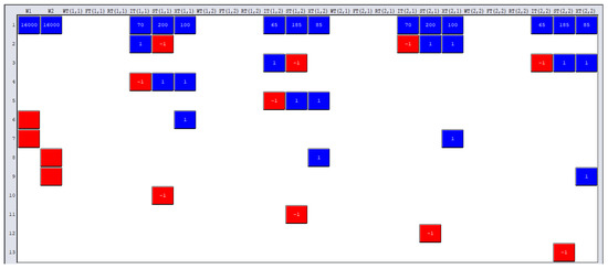
Figure 1.
Matrix structure of the developed models, developed in LINGO 19.0.
4.1. Results
For the solution of the deterministic equivalent of the multi-stage stochastic programming model, a Dell Inspiron 5570 computer with an Intel1 Core™ i5-8250U processor, 1.6 GHz and 4 Gb RAM memory was used. The mathematical modeling language LINGO 19.0 was used with the Branch-and-Bound solver. For the relaxation of the problem four cores of the processors, simplex and dual-simplex algorithms were used. For the pre-integer solver, the maximum number of heuristics allowed in LINGO 19.0 was used (100). Constraint cuts were applied using all the ability options and both directions (up and down) were considered in the branching process. Other settings in the solver were in default; an example of report solution is in Appendix A.
In Table 2, the comparison between the size of the deterministic equivalent is shown. It is evident that when the number of scenarios increases, the size of the model also increases, which is because of the deterministic equivalent increase proportionality with respect to the increments in the number of stages and/or realizations of the random variable. Because the Branch-and-Bound solver is used, the number of branches also increases when the number of scenarios does, even if the maximum number of heuristics is used for pre-solving the problem.
Table 2.
Comparison of the size of the models developed.
For the solutions, we defined the here-and-now solution of the recourse problem (RP) as Equation (23), which indicates the optimal solution before the realization of the random vector . This approach seeks to find an optimal policy over all the possible scenarios in the stochastic programming model [26].
The wait-and-see solution, expressed as Equation (24), solves the expected value of the stochastic programming model. This solution considers that all the possible outcomes of the random vector are known, hence the non anticipativity constraints are dropped, in other words, the relaxation of the here-and-know solution [44].
For a minimized problem, it is clear that the wait-and-see solution always will be less or equal to the here-and-now solution, and in a maximized problem, the wait-and-see solution will be greater or equal to the here-and-now solution. These valid inequalities are important because the deterministic equivalent of the stochastic programming is complicated to solve under the here-and-now solution. A good alternative is to use the wait-and-see solution as an approach that only solves a deterministic problem by dropping the non anticipativity constraints.
Finally, the absolute difference between the RP solution and the WS solution is called the expected value for perfect information, denoted in Equation (25), which indicates the maximum amount that the decision maker is willing to pay to know the uncertainty in advance [26].
Table 3 indicates the input for the deterministic parameters in the multi-product AAP under uncertainty. The input values were used for solving the stochastic programming model with LINGO 19.0, and the model considers two families of products, each family having a demand and production capacity.
Table 3.
Input data for the stochastic programming model: inventory, production, backlog, workers costs and service level.
Table 4 indicates the input for the stochastic parameters in the multi-product AAP under uncertainty. The values were obtained with Gaussian quadrature, proposed by Miller and Rice [45]. The probabilities are the same for three discrete points and are 0.167, 0.66 and 0.167; meanwhile, in the case of four discrete points, they are 0.05, 0.45, 0.45 and 0.05. Here, indicates a family of products 1 and , a family of products 2.
Table 4.
Input data for the stochastic programming model: demand and production capacity.
In Table 5, the comparison of both multi-stages developed models with respect to the here-and-now (RP) and wait-and-see approach (WS) is shown, as well as the expected value for perfect information (EVPI). Finally, CPU time and the number of iterations for solving each problem are reported. Here, it is clear that the second proposal model is more efficient and tractable for the solver. Appendix A shows the solution of Model-IIb in Lingo.
Table 5.
Comparison of the results of the models developed.
From Table 5, it is noted that the RP solution was the same for all the cases; however, the WS solution changes and, therefore, the EVPI. In Model-IIa and Model-IIb, the WS solutions were higher than Model-Ia and Model-IIb, respectively, which reduced the EVPI for the models with bounds, and then, the uncertainty was reduced. This has sense since we made a bound in the decision variables. On the other hand, the advantage when the bounds were used is noticed in the CPU time and iterations needed to solve the problems. For example, Model-Ib required more than half a million iterations and nearly 11 min for solving the deterministic equivalent, and Model-IIb only took less than 6 min and nearly 150 thousand iterations.
In Figure 2, the percentage GAP between Model-Ia versus Model-IIa and Model-Ib versus Model-IIb is compared. The CPU time GAP was calculated, as Equation (26), and it is noted when the model increases in size, the use of the upper and lower bounds in the first-stage decision variables decreases to 52.38% of the CPU time when four possible realizations of random variables occur.
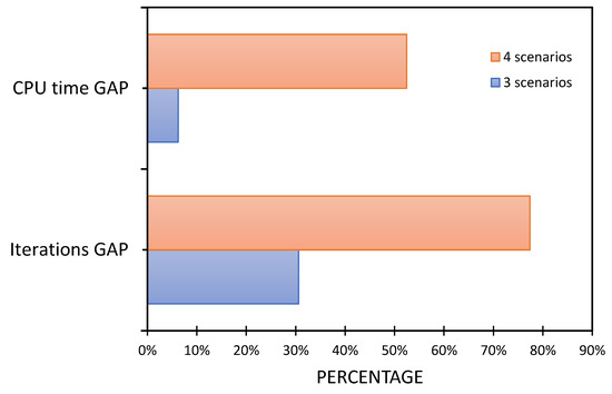
Figure 2.
Percentage GAP in CPU time and iterations for the developed models.
Equation (27) calculated the iterations GAP, and it is noted when the model increases in size, the use of the upper and lower bounds in first-stage decision variables decreases in more than 78.16% of the number of iterations.
When the model only considers three possible outcomes of the random variables, the advantage is even noted because the iterations were reduced by around 31% and the CPU time by 6%. This indicates that the use of bounds in decision variables improves the speed for solving the stochastic programming models.
4.2. Sensitivity Analysis
In this section, a sensitivity analysis was carried out considering how the percentage of the level service affects the solutions of the models. In this study, we changed the percentage of the level service from 85% to 95% for both families of products, and then, the stochastic programming model was solved and Model-Ia was used.
In Table 6, it is noted that a higher-level service increases the RP solution and the WS solution; however, the increment of the EVPI indicates that there exists more uncertainty when the level service increases; therefore, when the level service increases, it is better to have a good fit approximation of the random parameters, hence good quality of data is required.
Table 6.
Sensitivity analysis developed varying levels of service. * Denotes base case.
The increase is reasonable due to the fact that more workers are required to fulfill the percentage of the demand required. This sensitivity analysis also indicates how the workforce may change when the level of service policy changes. Similarly, the reported solutions can be used as an alternative for evaluating a better level services policy without the use of an objective that maximizes this percentage, as stated by Jamalnia et al. [1], where this only increases the complexity of the model making it difficult to solve in the here-and-now approach and, hence, difficult to apply and understand in real cases.
5. Conclusions
In this study, we proposed a new mathematical stochastic multi-stage programming model for solving real aggregate production planning under uncertainty. A previous work considering a one-product model was extended since the deterministic equivalent was difficult to solve and the matrix structure of the model made it difficult to use other algorithms such as Branch-and-Price. For that reason, bounds were proposed for the first-stage decision variables including the mathematical demonstration.
The reported solutions indicate that the use of bounds in the model is better because it decreases the number of iterations and CPU time and the solution is the same. This is because the use of bounds reduced the search space of the branching process during the Branch-and-Bound algorithm, and, therefore, the model is solved more efficiently.
Finally, a sensitivity analysis was performed to understand how the level of service impacted the RP and WS solutions in the model. We found that EVPI escalates when the level service increases; therefore, the uncertainty of the model increases when the level of service increases.
The use of the structure of the problem and making some bounds in decision variables are recommended because it implies fewer iterations and a lower CPU time. In this approach, it is demonstrated how the model increases in size when the number of possible outcomes of random variables increases.
This allows for having enough discrete points to make the model more tractable and hence, to implement it more easily in real industry problems. Further research could consider finding bounds in other decision variables to improve the model as well as another structure formulation of the mathematical model in order to use a different algorithm such as Branch-and-Prince, which is a method also available in LINGO 19.0. Similarly, it is re-commended to deal with uncertainty in different variables and additionally, incorporate supply chain decisions [5] and environmental and social issues [46,47] with sustainability.
Author Contributions
Conceptualization, J.E.G.-R. and E.S.H.-G.; methodology, J.E.G.-R.; software, J.E.G.-R.; validation, E.S.H.-G.; formal analysis, E.S.H.-G.; investigation, J.E.G.-R. and E.S.H.-G.; data curation, E.S.H.-G.; writing—original draft preparation, J.E.G.-R. and E.S.H.-G.; writing—review and editing, E.S.H.-G.; supervision, E.S.H.-G. All authors have read and agreed to the published version of the manuscript.
Funding
This research received no external funding.
Conflicts of Interest
The authors declare no conflict of interest.
Appendix A
Figure A1 is a report solution for Model-IIb. The objective value reports the RP solution, and objective bound indicates the theoretical solution of the mixed integer linear programming (MILP). Notice in this case that the objective value and the objective bound were the same; hence, the GAP was 0% in the MILP. Infeasibilities report how many constraints were violated, and extended solver steps indicate the number of branches in the Branch-and-Bound tree.
Total solver iterations and elapsed runtime seconds illustrate the values that are reported in Table 3. The expected value of the objective is the RP solution, and Deteq Model Class indicates the model class of the deterministic equivalent, in this case, a MILP. Total scenarios indicate the number of scenarios in the deterministic equivalent, and total random variables reported the number of random variables in the model. Total stages indicate how many stages have the stochastic programming model; we mentioned that LINGO 19.0 reports two due to the fact that the first stage is reported in LINGO 19.0 as stage 0; hence, this model has three stages.
Finally, the total variables, total constraints and total nonzeros reported the solution for both the deterministic model (Core) and the deterministic equivalent of the stochastic programming model (Deteq).

Figure A1.
Example of report solution for Model-IIb, developed in LINGO 19.0.
Figure A1.
Example of report solution for Model-IIb, developed in LINGO 19.0.

References
- Mina-Casaran, J.D.; Echeverry, D.F.; Lozano, C.A.; Navarro-Espinosa, A. On the Value of Community Association for Microgrid Development: Learnings from Multiple Deterministic and Stochastic Planning Designs. Appl. Sci. 2021, 11, 6257. [Google Scholar] [CrossRef]
- Yu, V.F.; Kao, H.-C.; Chiang, F.-Y.; Lin, S.-W. Solving Aggregate Production Planning Problems: An Extended TOPSIS Approach. Appl. Sci. 2022, 12, 6945. [Google Scholar] [CrossRef]
- Krajčovič, M.; Furmannová, B.; Grznár, P.; Furmann, R.; Plinta, D.; Svitek, R.; Antoniuk, I. System of Parametric Modelling and Assessing the Production Staff Utilisation as a Basis for Aggregate Production Planning. Appl. Sci. 2021, 11, 9347. [Google Scholar] [CrossRef]
- Gansterer, M. Aggregate planning and forecasting in make-to-order production systems. Int. J. Prod. Econ. 2015, 170, 521–528. [Google Scholar] [CrossRef]
- Pérez-Salazar, M.d.R.; Aguilar-Lasserre, A.A.; Cedillo-Campos, M.G.; Posada-Gómez, R.; del Moral-Argumedo, M.J.; Hernández-González, J.C. An Agent-Based Model Driven Decision Support System for Reactive Aggregate Production Scheduling in the Green Coffee Supply Chain. Appl. Sci. 2019, 9, 4903. [Google Scholar] [CrossRef]
- Sereshti, N.; Adulyasak, Y.; Jans, R. The value of aggregate service levels in stochastic lot sizing problems. Omega 2021, 102, 102335. [Google Scholar] [CrossRef]
- Darvishi, F.; Yaghin, R.G.; Sadeghi, A. Integrated fabric procurement and multi-site apparel production planning with cross-docking: A hybrid fuzzy-robust stochastic programming approach. Appl. Soft Comput. 2020, 92, 106267. [Google Scholar] [CrossRef]
- Jalanko, M.; Mahalec, V. Gasoline Blend Planning under Demand Uncertainty: Aggregate Supply–Demand Pinch Algorithm with Rolling Horizon. Ind. Eng. Chem. Res. 2019, 59, 281–298. [Google Scholar] [CrossRef]
- Zaidan, A.A.; Atiya, B.; Abu Bakar, M.R.; Zaidan, B.B. A new hybrid algorithm of simulated annealing and simplex downhill for solving multiple-objective aggregate production planning on a fuzzy environment. Neural Comput. Appl. 2019, 31, 1823–1834. [Google Scholar] [CrossRef]
- Wang, S.C.; Yeh, M.F. A modified particle swarm optimization for aggregate production planning. Expert Syst. Appl. 2014, 41, 3069–3077. [Google Scholar] [CrossRef]
- Cheraghalikhani, A.; Khoshalhan, F.; Mokhtari, H. Aggregate production planning: A literature review and future research directions. Int. J. Ind. Eng. Comput. 2019, 10, 309–330. [Google Scholar] [CrossRef]
- Mehdizadeh, E.; Niaki, S.T.A.; Hemati, M. A bi-objective aggregate production planning problem with learning effect and machine deterioration: Modeling and solution. Comput. Oper. Res. 2018, 91, 21–36. [Google Scholar] [CrossRef]
- Xue, G.; Offodile, F. Integrated optimization of dynamic cell formation and hierarchical production planning problem. Comput. Ind. Eng. 2020, 139, 106155. [Google Scholar] [CrossRef]
- Erfanian, M.; Pirayesh, M. Integration aggregate production planning and maintenance using mixed integer linear programming. In Proceedings of the 2016 IEEE International Conference on Industrial Engineering and Engineering Management, Bali, Indonesia, 4–7 December 2016; pp. 927–930. [Google Scholar] [CrossRef]
- Jamalnia, A.; Yang, J.B.; Feili, A.; Xu, D.L.; Jamali, G. Aggregate production planning under uncertainty: A comprehensive literature survey and future research directions. J. Adv. Manuf. Technol. 2019, 102, 159–181. [Google Scholar] [CrossRef]
- Gómez-Rocha, J.E.; Hernández-Gress, E.S.; Rivera-Gómez, H. Production planning of a furniture manufacturing company with random demand and production capacity using stochastic programming. PLoS ONE 2021, 16, e0252801. [Google Scholar] [CrossRef] [PubMed]
- Huselid, M.A. The impact of human resource management practices on turnover, productivity, and corporate financial performance. Acad. Manag. J. 1995, 38, 635–672. [Google Scholar] [CrossRef]
- Thomas, L.J.; McClain, J.O. An overview of production planning. Handb. Oper. Res. Manag. Sci. 1993, 4, 333–370. [Google Scholar] [CrossRef]
- Jamalnia, A.; Feili, A. A simulation testing and analysis of aggregate production planning strategies. Prod. Plan. Control. 2013, 24, 423–448. [Google Scholar] [CrossRef]
- Li, B.; Wang, H.; Yang, J.; Guo, M.; Qi, C. A belief-rule-based inference method for aggregate production planning under uncertainty. Int. J. Prod. Res. 2013, 51, 83–105. [Google Scholar] [CrossRef]
- Gholamian, N.; Mahdavi, I.; Tavakkoli-Moghaddam, R.; Mahdavi-Amiri, N. Comprehensive fuzzy multi-objective multi-product multi-site aggregate production planning decisions in a supply chain under uncertainty. Appl. Soft Comput. 2015, 37, 585–607. [Google Scholar] [CrossRef]
- Gholamian, N.; Mahdavi, I.; Tavakkoli-Moghaddam, R. Multi-objective multi-product multi-site aggregate production planning in a supply chain under uncertainty: Fuzzy multi-objective optimisation. Int. J. Comput. Integr. Manuf. 2016, 29, 149–165. [Google Scholar] [CrossRef]
- Aliev, R.A.; Fazlollahi, B.; Guirimov, B.G.; Aliev, R.R. Fuzzy-genetic approach to aggregate production–distribution planning in supply chain management. Inform. Sci. 2007, 177, 4241–4255. [Google Scholar] [CrossRef]
- Jamalnia, A.; Yang, J.B.; Xu, D.L.; Feili, A. Novel decision model based on mixed chase and level strategy for aggregate production planning under uncertainty: Case study in beverage industry. Comput. Ind. Eng. 2017, 114, 54–68. [Google Scholar] [CrossRef]
- Miettinen, K.; Mäkelä, M.M. Synchronous Approach in Interactive Multiobjective Optimization. Eur. J. Oper. Res. 2006, 170, 909–922. [Google Scholar] [CrossRef]
- Zhao, H.; Huang, E.; Dou, R.; Wu, K. A multi-objective production planning problem with the consideration of time and cost in clinical trials. ESWA 2019, 124, 25–38. [Google Scholar] [CrossRef]
- Chen, Y.K.; Liao, H.C. An investigation on selection of simplified aggregate production planning strategies using MADM approaches. Int. J. Prod. Res. 2003, 41, 3359–3374. [Google Scholar] [CrossRef]
- Kazemi Zanjani, M.; Nourelfath, M.; Aït-Kadi, D. Production planning with uncertainty in the quality of raw materials: A case in sawmills. J. Oper. Res. Soc. 2011, 62, 1334–1343. [Google Scholar] [CrossRef]
- Kazemi Zanjani, M.; Ait-Kadi, D.; Nourelfath, M. A stochastic programming approach for sawmill production planning. Int. J. Math. Oper. Res. 2013, 5, 1–18. [Google Scholar] [CrossRef]
- Huang, K. Multi-Stage Stochastic Programming Models for Production Planning. Ph.D. Thesis, School of Industrial and Systems Engineering, Georgia Institute of Technology, Atlanta, GA, USA, 2005. [Google Scholar]
- Mirzapour Al-e-hashem, S.M.J.; Baboli, A.; Sazvar, Z. A stochastic aggregate production planning model in a green supply chain: Considering flexible lead times, nonlinear purchase and shortage cost functions. Eur. J. Oper. Res 2013, 230, 26–41. [Google Scholar] [CrossRef]
- Nasiri, G.R.; Davoudpour, H.; Movahedi, Y. A Genetic Algorithm Approach for the Multi-commodity, Multi-period Distribution Planning in a Supply Chain Network Design. In Swarm, Evolutionary, and Memetic Computing. SEMCCO 2010. Lecture Notes in Computer Science; Panigrahi, B.K., Das, S., Suganthan, P.N., Dash, S.S., Eds.; Springer: Berlin/Heidelberg, Germany, 2010; Volume 6466, pp. 494–505. [Google Scholar] [CrossRef]
- Nasiri, G.R.; Davoudpour, H.; Karimi, B. The impact of integrated analysis on supply chain management: A coordinated approach for inventory control policy. Supply Chain. Manag. 2010, 15, 277–289. [Google Scholar] [CrossRef]
- Nasiri, G.R.; Zolfaghari, R.; Davoudpour, H. An integrated supply chain production–distribution planning with stochastic demands. Comput. Ind. Eng. 2014, 77, 35–45. [Google Scholar] [CrossRef]
- Ning, Y.; Liu, J.; Yan, L. Uncertain aggregate production planning. Soft Comput. 2013, 17, 617–624. [Google Scholar] [CrossRef]
- Lieckens, K.; Vandaele, N. A Decision Support System for the Stochastic Aggregate Planning Problem. 2014. Available online: https://ssrn.com/abstract=2419376 (accessed on 28 March 2014).
- Hu, Z.; Hu, G. A multi-stage stochastic programming for lot-sizing and scheduling under demand uncertainty. Comput. Ind. Eng. 2018, 119, 157–166. [Google Scholar] [CrossRef]
- Körpeoglu, E.; Yaman, H.; Aktürk, M.S. A multi-stage stochastic programming approach in master production scheduling. Eur. J. Oper. Res. 2011, 213, 166–179. [Google Scholar] [CrossRef]
- Leung, S.C.H.; Wu, Y. A robust optimization model for stochastic aggregate production planning. Prod. Plan. Control 2004, 15, 502–514. [Google Scholar] [CrossRef]
- Kanyalkar, A.P.; Adil, G.K. A robust optimization model for aggregate and detailed planning of a multi-site procurement-production-distribution system. Int. J. Prod. Res. 2010, 48, 635–656. [Google Scholar] [CrossRef]
- Mirzapour Al-e-hashem, S.M.J.; Malekly, H.; Aryanezhad, M.B. A multi-objective robust optimization model for multi-product multi-site aggregate production planning in a supply chain under uncertainty. Int. J. Prod. Econ. 2011, 134, 28–42. [Google Scholar] [CrossRef]
- Mirzapour Al-e-hashem, S.M.J.; Aryanezhad, M.B.; Sadjadi, S.J. An efficient algorithm to solve a multi-objective robust aggregate production planning in an uncertain environment. Int. J. Adv. Manuf. Technol. 2012, 58, 765–782. [Google Scholar] [CrossRef]
- Makui, A.; Heydari, M.; Aazami, A.; Dehghani, E. Accelerating Benders decomposition approach for robust aggregate production planning of products with a very limited expiration date. Comput. Ind. Eng. 2016, 100, 34–51. [Google Scholar] [CrossRef]
- Birge, J.R.; Louveaux, F. Introduction to Stochastic Programming; Springer: New York, NY, USA, 1997. [Google Scholar]
- Miller, A.C., III; Rice, T.R. Discrete approximations of probability distributions. Manag. Sci. 1983, 29, 352–362. [Google Scholar] [CrossRef]
- Türkay, M.; Saraçoğlu, Ö.; Arslan, M.C. Sustainability in Supply Chain Management: Aggregate Planning from Sustainability Perspective. PLoS ONE 2016, 11, e0147502. [Google Scholar] [CrossRef] [PubMed]
- Yaghin, R.G.; Sarlak, P.; Ghareaghaji, A. Robust master planning of a socially responsible supply chain under fuzzy-stochastic uncertainty (A case study of clothing industry). Eng. Appl. Artif. Intell. 2020, 94, 103715. [Google Scholar] [CrossRef]


Publisher’s Note: MDPI stays neutral with regard to jurisdictional claims in published maps and institutional affiliations. |
© 2022 by the authors. Licensee MDPI, Basel, Switzerland. This article is an open access article distributed under the terms and conditions of the Creative Commons Attribution (CC BY) license (https://creativecommons.org/licenses/by/4.0/).