Three-Dimensional Analytical Calculation and Optimization of Plate-Type Permanent Magnet Electrodynamic Suspension System

Abstract

With the development of rare earth permanent magnet (PM) materials, more and more attention has been paid to the permanent magnet electrodynamic suspension (PM-EDS) structure. In this paper, the plate-type PM-EDS structure with an adjustable deflection angle of PM is researched, and the size of the PM is optimized. First, the second-order vector potential (SOVP) equation is established, and the analytical solutions of the electromagnetic forces and magnetic fields of the PM-EDS structure are obtained by analytical calculation. Secondly, the accuracy and reliability of the analytical model are verified by comparing the analytical calculation results with the finite element analysis (FEA) calculation results. Finally, the multi-objective particle swarm optimization (MOPSO) algorithm is used to optimize the size of the PM. The optimization results prove that the lift-to-drag ratio and lift-to-weight ratio of the suspension system are improved. The research results can provide a theoretical basis for the design of a PM-EDS train.

1. Introduction

The plate-type PM-EDS system is mainly composed of PMs and nonmagnetic conductive plates. By the relative motion between the PMs and the conductive plates, induction eddy currents are formed in the conductive plates, which interact with the source of the magnetic field to generate the electromagnetic force to suspend the PMs [1]. PM-EDS system has the advantages of no friction, low power consumption, large levitation air gap and simple structure. Typical PM-EDS systems include the Magplane system [2,3], the InductrackII system [4] and the Skytran system [5,6]. The design speed of the Magplane vehicle is 250 km/h, its conductive plate is approximately arc-shaped, and the on-board Halbach PM arrays are used as the magnetic excitation sources as shown in Figure 1, which has low cost and high reliability, but the drag force is too large and the lift-to-drag ratio is low at low speed. As shown in Figure 2, the characteristic of the InductrackII system is that there are a set of Halbach PM arrays on the upper and lower sides of the conductive plate, respectively, which makes the drag force smaller at low speed, but it is not suitable for high-speed operation. As shown in Figure 3, the Skytran system places the conductive plate vertically, and the levitation force is generated by the angle between the PM and the conductive plate. The structure of Skytran mainly includes four parts: on-board PMs, propulsion system, ground track system and vehicle cabin. The linear propulsion motor pulls the train along the track, and suspension force is generated between the PMs and the conductive plates; the support wheels provide support when the train is not suspended.

Although the PM-EDS system can be self-stabilizing, the system damping is weak and even exhibits a negative damping state under certain conditions. Therefore, the active damping or passive damping scheme is necessary. To improve the damping, the Magplane system adopts the active control of adjusting the magnet position by a set of hydraulic systems [7]. The InductrackII system uses a hybrid magnetic array with PMs and electromagnetic coils to realize the active control of the levitation force of the train by dynamically adjusting the current in the coil. The PM of the Skytran system can be driven by a motor to rotate around the shaft, and the levitation force can be dynamically adjusted by adjusting the angle between the PM and the conductive plate. The Skytran system, with adjustable angles of PMs, provides more flexibility. However, compared with Magplane and InductrackII systems, the angle adjustment mechanism will lead to increased weight and fatigue wear of the suspension system. At the same time, the problem of a small lift-to-drag ratio and lift-to-weight ratio of the PM-EDS system cannot be ignored [8].

The structure of Skytran is introduced in detail in articles [5,6]. However, there is no article that calculates the electromagnetic forces and magnetic fields of Skytran system. The innovation of this paper is that the analytical calculation of electromagnetic forces and magnetic fields of the PM-EDS structure with an adjustable angle of PM is derived in detail, and the size of the PM is optimized by using the MOPSO method. First, the electromagnetic field analytical model of the system is established by introducing the SOVP, and the analytical solutions of the electromagnetic forces and the magnetic fields are obtained from the boundary conditions. Secondly, the FEA simulation model of the PM-EDS structure is established, and the calculation results of the analytical solution are verified. The results show that the calculation results of the two methods are consistent. Finally, the length, width and thickness of the PM are optimized to maximize the lift-to-drag ratio and lift-to-weight ratio by using the MOPSO algorithm. A Pareto solution set of the optimal solutions is obtained, and a solution with the best comprehensive performance is selected from the Pareto set by using fuzzy set theory. This paper provides a systematic, accurate and general analysis method for PM-EDS trains.

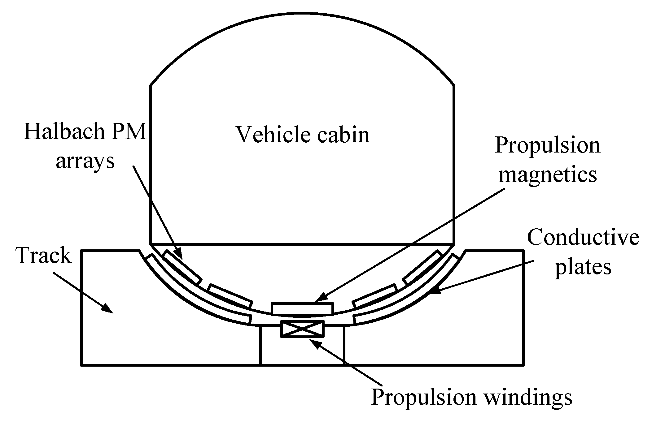
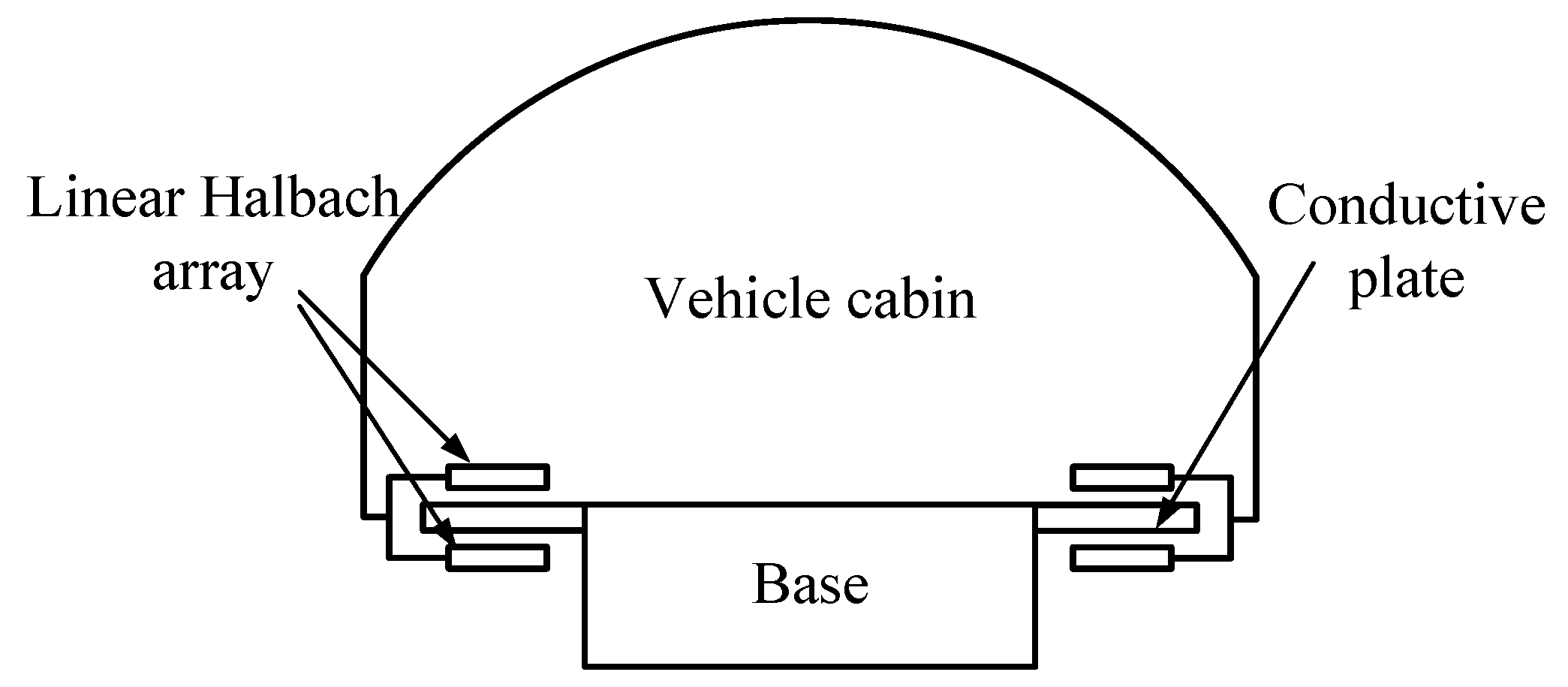
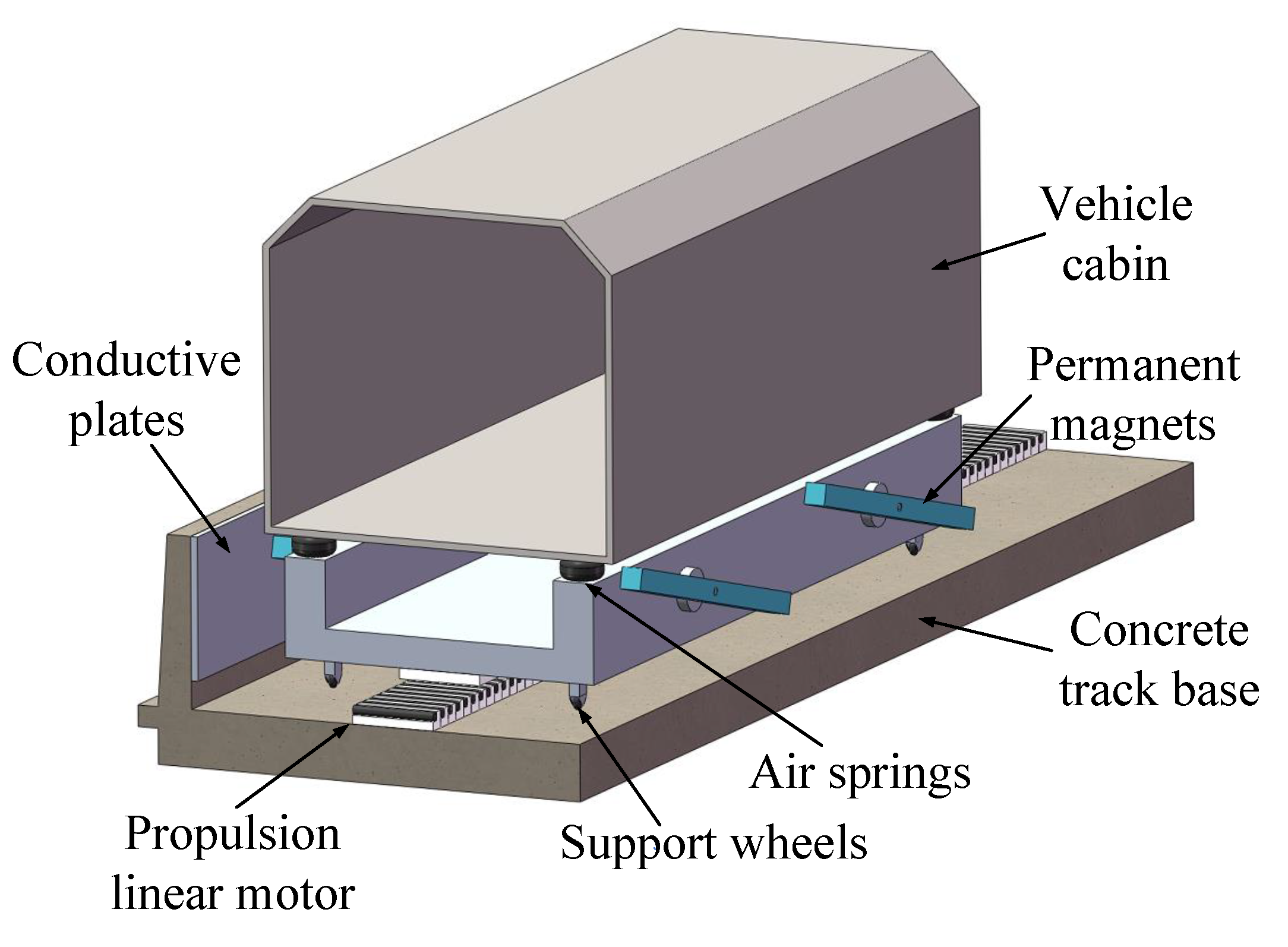
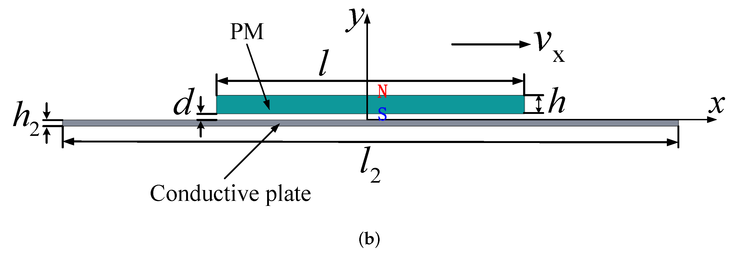
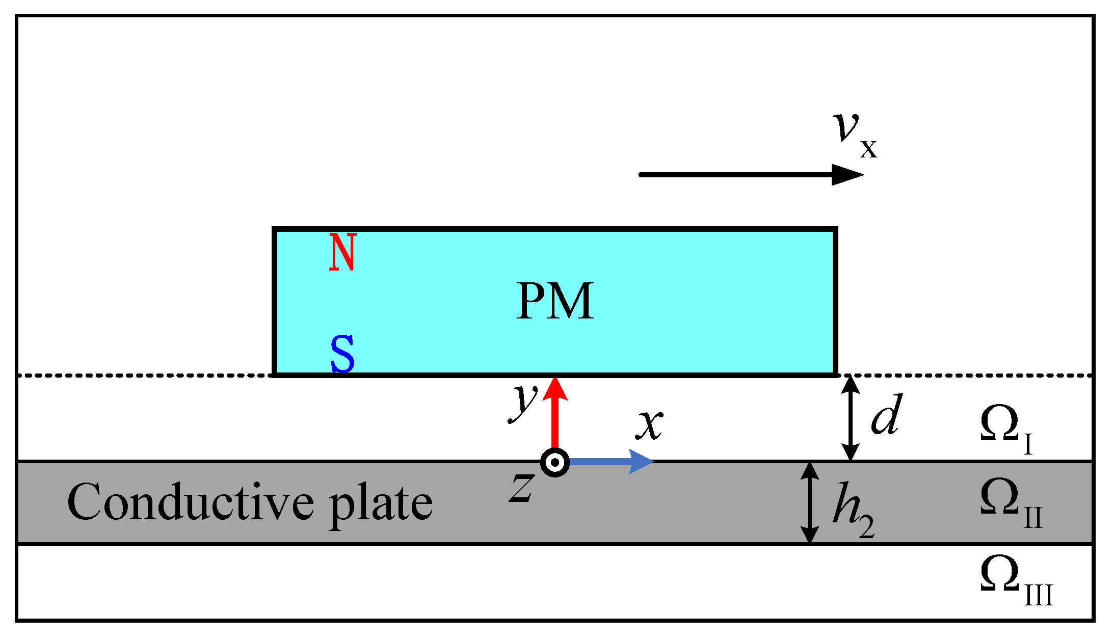
2. Structure of the Suspension System

The 3-D and 2-D schematics of the suspension system structure are shown in Figure 4, which consists of a PM and nonmagnetic conductive plate. In Figure 4a, the PM moves along the x-positive direction at a speed $v_{\mathrm{x}}$, the angle between the PM and the center line of the conductive plate is $\theta$, the width of the PM is w and the width of the conductive plate is $w_2$. In Figure 4b, l and h are the length and thickness of the PM, respectively, $l_2$ and $h_2$ are the length and thickness of the conductive plate, respectively, the air gap between the PM and the conductive plate is d, and the magnetization direction of the PM is along the y-positive direction. During the movement, the PM is subjected to levitation force $F_{\mathrm{z}}$, drag force $F_{\mathrm{x}}$ and lateral force $F_{\mathrm{y}}$.

3. Analytical Model Calculation and Validation

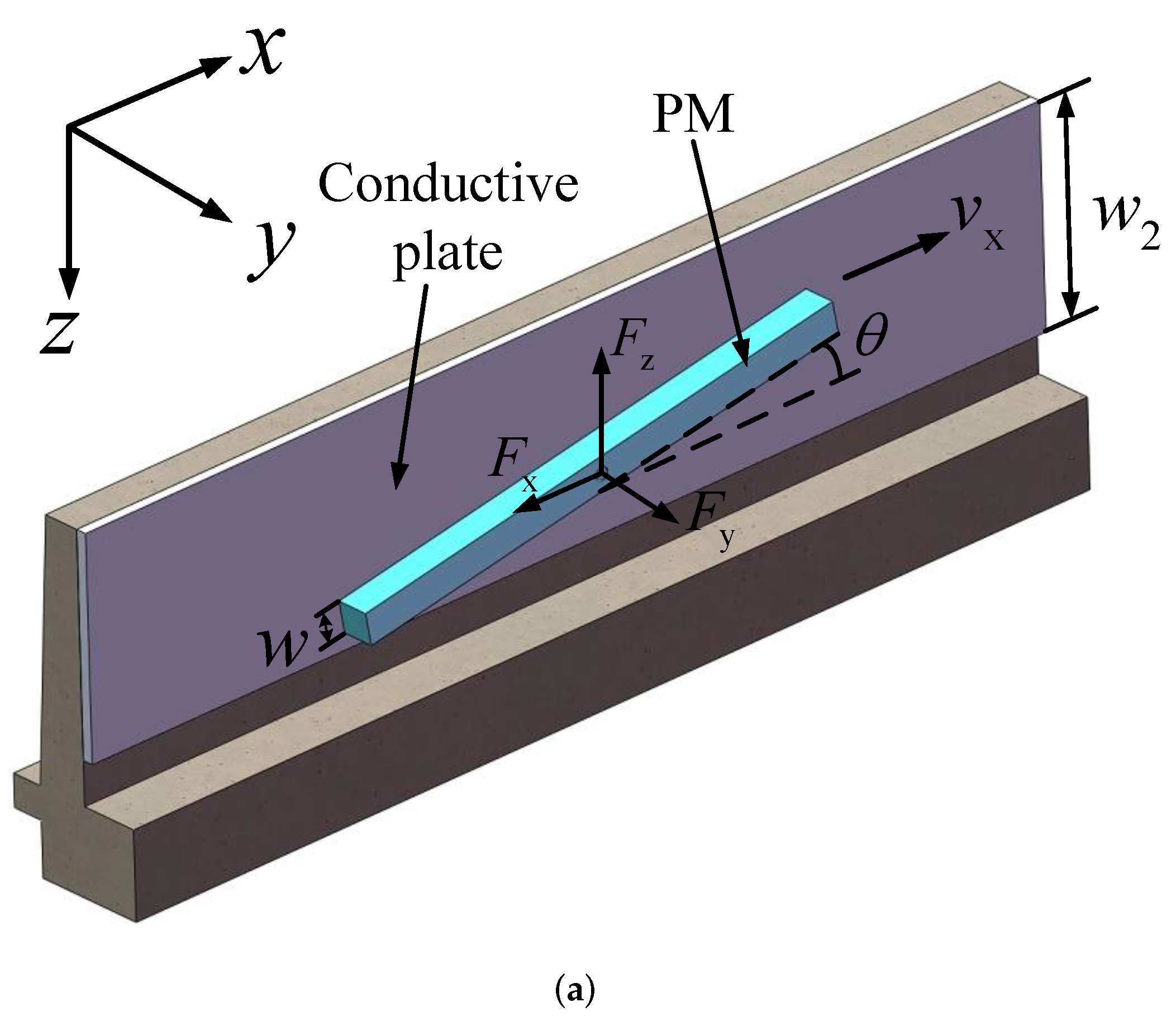
3.1. Analytical Calculation

3.1.1. Establishment of Equation

The space region in Figure 4b is divided into three parts [9], as shown in Figure 5. Region I (${\mathsf{\Omega }}_{\mathrm{I}}$) is the nonconductive region between the PM and the conductive plate with a coordinate range $0<y<d$, region II (${\mathsf{\Omega }}_{\mathrm{II}}$) is the conductive region with a coordinate range $-h_2<y<0$, and region III (${\mathsf{\Omega }}_{\mathrm{III}}$) is the nonconductive region below the conductive plate with a coordinate range $y<-h_2$.

The assumptions of this analytic model are listed below:

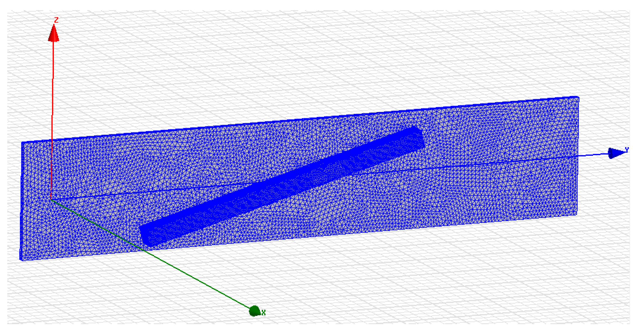
• The length $l_2$ and width $w_2$ of the conductive plate are large enough to be regarded as infinite, and the thickness $h_2$ is finite.
• The conductive plate is continuous with constant conductivity and is nonmagnetic.
• The PM can move translationally along the x, y and z-axes.
• The moving speed of the PM is much less than the speed of light, which makes the frequency of the magnetic field low enough, and the system approximates a quasi-static model.

Using the SOVP to calculate the model. The SOVP is expressed as W and is defined as [10]:

$$B=\nabla \times A=\nabla \times \nabla \times W$$

(1)

where B is the magnetic flux density, and A is the magnetic vector potential. W can be split into two components of transverse electric (TE) and transverse magnetic (TM) in the y-direction as follows [11]:

$$W=\overrightarrow{y}{W}_{\mathrm{a}}+\overrightarrow{y}\times \nabla W_{\mathrm{b}}$$

(2)

where $\overrightarrow{y}$ is the unit vector along the y-direction, and $W_{\mathrm{a}}$ and $W_{\mathrm{b}}$ are the TE and TM potential, respectively. Substituting Equation (2) into Equation (1) gives:

$$\begin{array}{cc}& A_{\mathrm{x}}=-\frac{\partial W_{\mathrm{a}}}{\partial z}-\frac{\partial W_{\mathrm{b}}}{\partial x\partial y}\\ & A_{\mathrm{y}}=\frac{{\partial }^2{W}_{\mathrm{b}}}{\partial x}+\frac{{\partial }^2{W}_{\mathrm{b}}}{\partial z^2}\\ & A_{\mathrm{z}}=\frac{\partial W_{\mathrm{a}}}{\partial x}-\frac{{\partial }^2{W}_{\mathrm{b}}}{\partial z\partial y}\end{array}$$

(3)

It is noticed that the $A_{\mathrm{y}}$ in Equation (3) is a function of $W_{\mathrm{b}}$ only because the unit vector of Equation (2) is chosen along the y-direction. Since it is assumed that the conductive plate is infinite, the eddy current generated in the conductive plate is always parallel to the upper surface of the conductive plate, and the $A_{\mathrm{y}}$ component is zero. Therefore, $W_{\mathrm{b}}$ is always zero. There is only a TE component in the SOVP; then Equation (2) can be written as:

$$W=\overrightarrow{y}{W}_{\mathrm{a}}$$

(4)

In the conductive region, the governing equation for the conductive plate in terms of the magnetic vector potential satisfies Equation (5):

$${\nabla }^{2}A={\mu }_0\sigma \left(-v_{\mathrm{x}}\frac{\partial A}{\partial x}-v_{\mathrm{y}}\frac{\partial A}{\partial y}-v_{\mathrm{z}}\frac{\partial A}{\partial z}\right)$$

(5)

where ${\mu }_0$ is the magnetic permeability of the vacuum, $\sigma$ is the conductivity of the conductive plate and $v_{\mathrm{x}}$, $v_{\mathrm{y}}$, $v_{\mathrm{z}}$ are the velocity of PM in the x, y and z-directions, respectively. Substituting Equation (1) and Equation (4) into Equation (5), we obtain the SOVP equation:

$$\frac{{\partial }^2{W}_{\mathrm{a}}}{\partial x^2}+\frac{{\partial }^2{W}_{\mathrm{a}}}{\partial y^2}+\frac{{\partial }^2{W}_{\mathrm{a}}}{\partial z^2}={\mu }_0\sigma \left(-v_{\mathrm{x}}\frac{\partial W_{\mathrm{a}}}{\partial x}-v_{\mathrm{y}}\frac{\partial W_{\mathrm{a}}}{\partial y}-v_{\mathrm{z}}\frac{\partial W_{\mathrm{a}}}{\partial z}\right)$$

(6)

Since the conductivity is zero in the nonconductive regions ${\mathsf{\Omega }}_{\mathrm{I}}$ and ${\mathsf{\Omega }}_{\mathrm{III}}$, from Equation (6) the TE potential satisfies the following equation:

$$\begin{array}{c}{\nabla }^2{W}_{\mathrm{a}}^{\mathrm{I},\mathrm{s}}=0\\ {\nabla }^2{W}_{\mathrm{a}}^{\mathrm{I},\mathrm{r}}=0\\ {\nabla }^2{W}_{\mathrm{a}}^{\mathrm{III}}=0\end{array}$$

(7)

and the TE potential in the conductive region ${\mathsf{\Omega }}_{\mathrm{II}}$ satisfies the following equation:

$${\nabla }^2{W}_{\mathrm{a}}^{\mathrm{II}}={\mu }_0\sigma \left(-v_{\mathrm{x}}\frac{\partial W_{\mathrm{a}}^{\mathrm{II}}}{\partial x}-v_{\mathrm{y}}\frac{\partial W_{\mathrm{a}}^{\mathrm{II}}}{\partial y}-v_{\mathrm{z}}\frac{\partial W_{\mathrm{a}}^{\mathrm{II}}}{\partial z}\right)$$

(8)

where $W_{\mathrm{a}}^{\mathrm{I},\mathrm{s}}$ and $W_{\mathrm{a}}^{\mathrm{I},\mathrm{r}}$ are the source and reflected TE potential in the region ${\mathsf{\Omega }}_{\mathrm{I}}$, respectively [12], $W_{\mathrm{a}}^{\mathrm{II}}$ is the total TE potential in the region ${\mathsf{\Omega }}_{\mathrm{II}}$ and $W_{\mathrm{a}}^{\mathrm{III}}$ is the transmitted TE potential in the region ${\mathsf{\Omega }}_{\mathrm{III}}$. These potentials are shown in Figure 6.

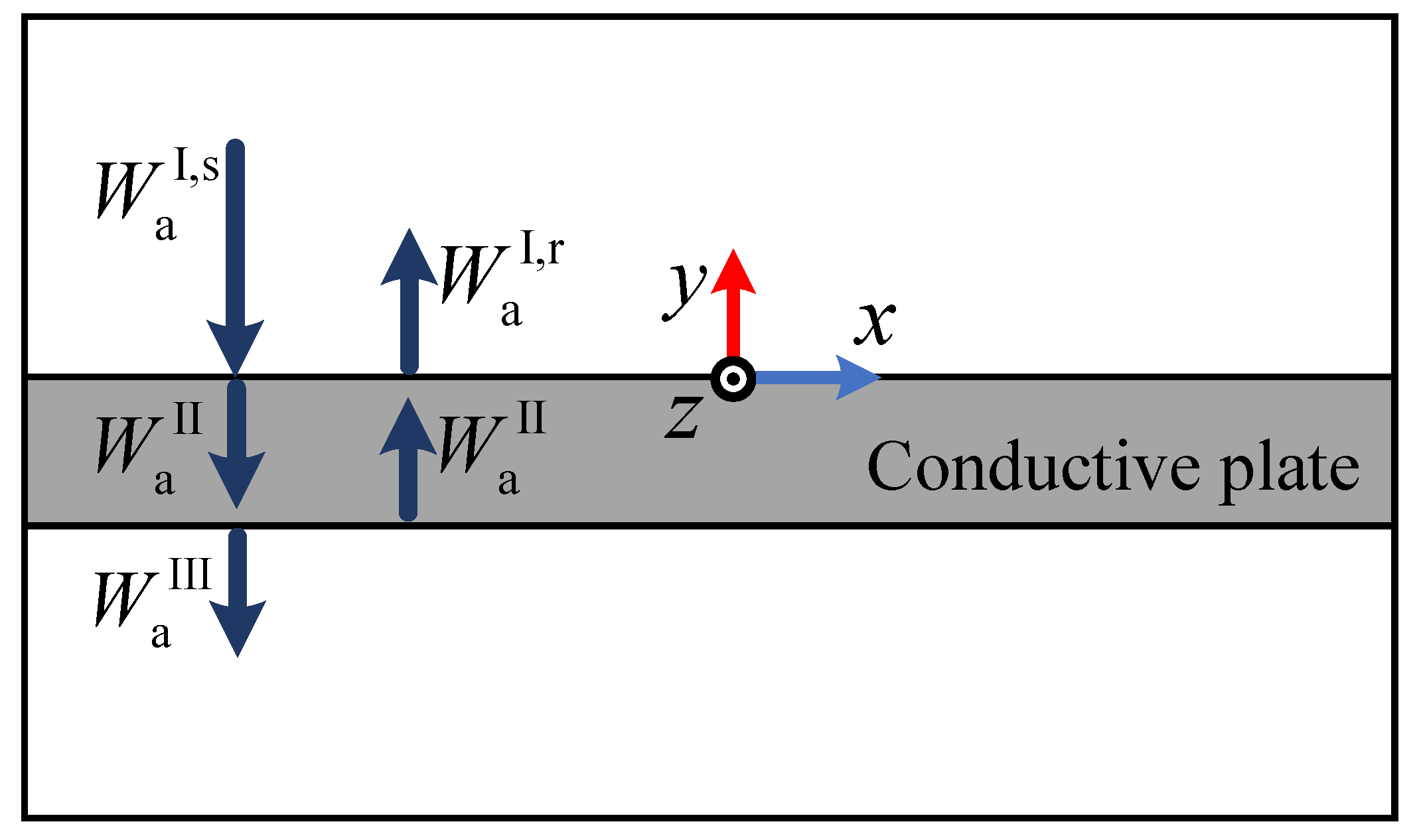
3.1.2. Boundary Conditions

The tangential component of the magnetic field strength and the normal component of the magnetic flux density must be continuous at the interface $y=0$ and $y=-h_2$; therefore, the boundary conditions are:

$$\begin{array}{cc}& B_{\mathrm{x}}^{\mathrm{I},\mathrm{s}}+B_{\mathrm{x}}^{\mathrm{I},\mathrm{r}}=B_{\mathrm{x}}^{\mathrm{II}},y=0\\ & B_{\mathrm{y}}^{\mathrm{I},\mathrm{s}}+B_{\mathrm{y}}^{\mathrm{I},\mathrm{r}}=B_{\mathrm{y}}^{\mathrm{II}},y=0\\ & B_{\mathrm{z}}^{\mathrm{I},\mathrm{s}}+B_{\mathrm{z}}^{\mathrm{I},\mathrm{r}}=B_{\mathrm{z}}^{\mathrm{II}},y=0\\ & B_{\mathrm{x}}^{\mathrm{II}}=B_{\mathrm{x}}^{\mathrm{III},\mathrm{t}},y=-h_2\\ & B_{\mathrm{y}}^{\mathrm{II}}=B_{\mathrm{y}}^{\mathrm{III},\mathrm{t}},y=-h_2\\ & B_{\mathrm{z}}^{\mathrm{II}}=B_{\mathrm{z}}^{\mathrm{III},\mathrm{t}},y=-h_2\end{array}$$

(9)

It is found that if Equation (9) holds, the TE potential and its normal derivative are continuous on the interface:

$$\begin{array}{cc}& W_{\mathrm{a}}^{\mathrm{I},\mathrm{s}}+W_{\mathrm{a}}^{\mathrm{I},\mathrm{r}}=W_{\mathrm{a}}^{\mathrm{II}},y=0\\ & \frac{\partial W_{\mathrm{a}}^{\mathrm{I},\mathrm{s}}}{\partial y}+\frac{\partial W_{\mathrm{a}}^{\mathrm{I},\mathrm{r}}}{\partial y}=\frac{\partial W_{\mathrm{a}}^{\mathrm{II}}}{\partial y},y=0\\ & W_{\mathrm{a}}^{\mathrm{II}}=W_{\mathrm{a}}^{\mathrm{III}},y=-h_2\\ & \frac{\partial W_{\mathrm{a}}^{\mathrm{II}}}{\partial y}=\frac{\partial W_{\mathrm{a}}^{\mathrm{III}}}{\partial y},y=-h_2\end{array}$$

(10)

Therefore, only the four boundary condition equations in Equation (10) need to be solved.

3.1.3. Solution of Equations

Using the separation of variables method, the TE potential in ${\mathsf{\Omega }}_{\mathrm{II}}$ can be expressed as [13]:

$$W_{\mathrm{a}}^{\mathrm{II}}\left(x,y,z\right)=\sum _{m=-M}^M\sum _{n=-N}^N{\mathrm{e}}^{j{\xi }_{m}x}{\mathrm{e}}^{j{k}_{n}z}\left(C_{mn}^{\mathrm{II}}{\mathrm{e}}^{{\alpha }_{mn}y}+D_{mn}^{\mathrm{II}}{\mathrm{e}}^{{\beta }_{mn}y}\right),-h_2<y<0$$

(11)

where M and N are harmonics of the Fourier series, ${\xi }_m=2\pi m/\phantom{2\pi m{l}_2}{l}_2$ and $k_n=2\pi n/\phantom{2\pi n{w}_2}{w}_2$ are spatial frequencies, $C_{mn}^{\mathrm{II}}$ and $D_{mn}^{\mathrm{II}}$ are the coefficients to be solved, ${\alpha }_{mn}$ and ${\beta }_{mn}$ are:

$${\alpha }_{mn}=0.5\left(-{\mu }_0\sigma v_{\mathrm{y}}+\sqrt{{\left({\mu }_0\sigma v_{\mathrm{y}}\right)}^2+4{{\gamma }_{mn}}^2}\right)$$

(12)

$${\beta }_{mn}=0.5\left(-{\mu }_0\sigma v_{\mathrm{y}}-\sqrt{{\left({\mu }_0\sigma v_{\mathrm{y}}\right)}^2+4{{\gamma }_{mn}}^2}\right)$$

(13)

where

$${{\gamma }_{mn}}^2={{\xi }_m}^2+{k_n}^2-j{\mu }_0\sigma \left(v_{\mathrm{x}}{\xi }_m+v_{\mathrm{z}}{k}_n\right)$$

(14)

Similarly, the TE potential in the region ${\mathsf{\Omega }}_{\mathrm{I}}$ and ${\mathsf{\Omega }}_{\mathrm{II}}$ can be obtained:

$$W_{\mathrm{a}}^{\mathrm{I},\mathrm{r}}\left(x,y,z\right)=\sum _{m=-M}^M\sum _{n=-N}^N{\mathrm{e}}^{j{\xi }_{m}x}{\mathrm{e}}^{j{k}_{\mathrm{n}}z}{C}_{mn}^{\mathrm{I},\mathrm{r}}{\mathrm{e}}^{-{\kappa }_{mn}y},0⩽y⩽d$$

(15)

$$W_{\mathrm{a}}^{\mathrm{III}}\left(x,y,z\right)=\sum _{m=-M}^M\sum _{n=-N}^N{\mathrm{e}}^{j{\xi }_{m}x}{\mathrm{e}}^{j{k}_{\mathrm{n}}z}{C}_{mn}^{\mathrm{III}}{\mathrm{e}}^{{\kappa }_{mn}\left(y+h_2\right)},y⩽-h_2$$

(16)

where

$${\kappa }_{mn}=\sqrt{{{\xi }_m}^2+{k_n}^2}$$

(17)

The analytical expression of the magnetic field generated by the PM can be obtained by Ampere’s molecular current hypothesis [14]; that is, the y component magnetic flux density generated by the PM at the upper surface of the conductive plate $B_{\mathrm{y}}^{\mathrm{s}}\left(x,0,z\right)$ is known. Then, the magnetic flux density in ${\mathsf{\Omega }}_{\mathrm{I}}$ can be expressed by a Fourier coefficient as [15]:

$$B_{\mathrm{y}}^{\mathrm{I},\mathrm{s}}\left(x,y,z\right)=\sum _{m=-M}^M\sum _{n=-N}^N{\mathrm{e}}^{j{\xi }_{m}x}{\mathrm{e}}^{j{k}_{n}y}{S}_{mn}^{\mathrm{I},\mathrm{s}}{\mathrm{e}}^{{\kappa }_{mn}y}$$

(18)

where $S_{mn}^{\mathrm{I},\mathrm{s}}$ is the Fourier coefficient, which can be calculated by Equation (19) or by the fast Fourier transform (FFT) more efficiently.

$$S_{mn}^{\mathrm{I},\mathrm{s}}=\frac{1}{l_2{w}_2}{\int }_{-w_2/\phantom{-w_{2}2}2}^{w_2/2}{\int }_{-l_2/2}^{l_2/2}{B}_{\mathrm{y}}^{\mathrm{s}}\left(x,0,z\right){\mathrm{e}}^{-j\left({\xi }_{m}x+k_{n}z\right)}\mathrm{d}x\mathrm{d}z$$

(19)

$W_{\mathrm{a}}^{\mathrm{I},\mathrm{s}}$ can be expressed by $B_{\mathrm{y}}^{\mathrm{I},\mathrm{s}}$ as

$$W_{\mathrm{a}}^{\mathrm{I},\mathrm{s}}\left(x,y,z\right)={\int }_{-\infty }^y{\int }_{-\infty }^y{B}_{\mathrm{y}}^{\mathrm{I},\mathrm{s}}\left(x,y,z\right)\mathrm{d}y\mathrm{d}y$$

(20)

Substituting Equation (18) into Equation (20), $W_{\mathrm{a}}^{\mathrm{I},\mathrm{s}}$ can be solved:

$$W_{\mathrm{a}}^{\mathrm{I},\mathrm{s}}\left(x,y,z\right)=\sum _{m=-M}^M\sum _{n=-N}^N{\mathrm{e}}^{j{\xi }_{m}x}{\mathrm{e}}^{j{k}_{n}z}{C}_{mn}^{\mathrm{I},\mathrm{s}}{\mathrm{e}}^{{\kappa }_{mn}y},0<y<d$$

(21)

where

$$C_{mn}^{\mathrm{I},\mathrm{s}}=\frac{1}{{{\kappa }_{mn}}^2}{S}_{mn}^{\mathrm{I},\mathrm{s}}$$

(22)

By taking Equation (11), Equation (15), Equation (16) and Equation (21) into the boundary conditions in Equation (10), four unknown coefficients, $C_{mn}^{\mathrm{II}}$, $D_{mn}^{\mathrm{II}}$, $C_{mn}^{\mathrm{I},\mathrm{r}}$ and $C_{mn}^{\mathrm{III}}$, can be solved. $C_{mn}^{\mathrm{II}}$ and $D_{mn}^{\mathrm{II}}$ are given as follows:

$$C_{mn}^{\mathrm{II}}=\frac{2{\kappa }_{mn}{C}_{mn}^{\mathrm{I},\mathrm{s}}\left({\beta }_{mn}-{\kappa }_{mn}\right){\mathrm{e}}^{-{\beta }_{mn}{h}_2}}{Q_{mn}}$$

(23)

$$D_{mn}^{\mathrm{II}}=\frac{-2{\kappa }_{mn}{C}_{mn}^{\mathrm{I},\mathrm{s}}\left({\alpha }_{mn}-{\kappa }_{mn}\right){\mathrm{e}}^{-{\alpha }_{mn}{h}_2}}{Q_{mn}}$$

(24)

where

$$Q_{mn}=\left(a_{mn}+{\kappa }_{mn}\right)\left({\beta }_{mn}-{\kappa }_{mn}\right){\mathrm{e}}^{-{\beta }_{mn}{h}_2}-\left({\beta }_{mn}+{\kappa }_{mn}\right)\left({\alpha }_{mn}-{\kappa }_{mn}\right){\mathrm{e}}^{-{\alpha }_{mn}{h}_2}$$

(25)

Substituting Equation (23), Equation (24) into Equation (11), the solution of TE potential in ${\mathsf{\Omega }}_{\mathrm{II}}$ is:

$$W_{\mathrm{a}}^{\mathrm{II}}\left(x,y,z\right)=\sum _{m=-M}^M\sum _{n=-N}^N{\mathrm{e}}^{j{\xi }_{m}x}{\mathrm{e}}^{j{k}_{n}z}{C}_{mn}^{\mathrm{I},\mathrm{s}}{T}_{mn}\left(y\right),-h_2<y<0$$

(26)

where

$$T_{mn}\left(y\right)=2{\kappa }_{mn}\left(\frac{\left({\beta }_{mn}-{\kappa }_{mn}\right){\mathrm{e}}^{\left({\alpha }_{mn}y-{\beta }_{mn}{h}_2\right)}-\left({\alpha }_{mn}-{\kappa }_{mn}\right){\mathrm{e}}^{\left({\beta }_{mn}y-{\alpha }_{mn}{h}_2\right)}}{Q_{mn}}\right)$$

(27)

By combining Equation (1), Equation (4) and Equation (26), the inducted magnetic flux density in conductive region ${\mathsf{\Omega }}_{\mathrm{II}}$ can be obtained as follows:

$$B_{\mathrm{x}}^{\mathrm{II}}\left(x,y,z\right)=\sum _{m=-M}^M\sum _{n=-N}^N\frac{j{\xi }_m}{{{\kappa }_{mn}}^2}{\mathrm{e}}^{j{\xi }_{m}x}{\mathrm{e}}^{j{k}_{n}z}{S}_{mn}^{\mathrm{I},\mathrm{s}}\frac{\mathrm{d}{T}_{mn}\left(y\right)}{\mathrm{d}y},-h⩽y⩽0$$

(28)

$$B_{\mathrm{y}}^{\mathrm{II}}\left(x,y,z\right)=\sum _{m=-M}^M\sum _{n=-N}^N{\mathrm{e}}^{j{\xi }_{m}x}{\mathrm{e}}^{j{k}_{n}z}{S}_{mn}^{\mathrm{I},\mathrm{s}}{T}_{mn}\left(y\right),-h⩽y⩽0$$

(29)

$$B_{\mathrm{z}}^{\mathrm{II}}\left(x,y,z\right)=\sum _{m=-M}^M\sum _{n=-N}^N\frac{j{k}_n}{{{\kappa }_{mn}}^2}{\mathrm{e}}^{j{\xi }_{m}x}{\mathrm{e}}^{j{k}_{n}z}{S}_{mn}^{\mathrm{I},\mathrm{s}}\frac{\mathrm{d}{T}_{mn}\left(y\right)}{\mathrm{d}y},-h⩽y⩽0$$

(30)

The drag, lateral and levitation forces acting on the conductive plate can be obtained by Maxwell’s stress tensor method [16], where ‘∗’ denotes a complex conjugate.

$$F_{\mathrm{x}}=\frac{1}{2{\mu }_0}Re\left\{{\int }_{-w_2/\phantom{-w_{2}2}2}^{w_2/2}{\int }_{-l_2/\phantom{-l_{2}2}2}^{l_2/\phantom{l_{2}2}2}{B}_{\mathrm{x}}^{\mathrm{II}}{B}_{\mathrm{y}}^{\mathrm{II}*}\mathrm{d}x\mathrm{d}z\right\}\left|{}_{y=0}\right.$$

(31)

$$F_{\mathrm{y}}=\frac{1}{4{\mu }_0}Re\left\{{\int }_{-w_2/\phantom{-w_{2}2}2}^{w_2/2}{\int }_{-l_2/\phantom{-l_{2}2}2}^{l_2/\phantom{l_{2}2}2}\left(B_{\mathrm{y}}^{\mathrm{II}}{B}_{\mathrm{y}}^{\mathrm{II}*}-B_{\mathrm{x}}^{\mathrm{II}}{B}_{\mathrm{x}}^{\mathrm{II}*}-B_{\mathrm{z}}^{\mathrm{II}}{B}_{\mathrm{z}}^{\mathrm{II}*}\right)\mathrm{d}x\mathrm{d}z\right\}\left|{}_{y=0}\right.$$

(32)

$$F_{\mathrm{z}}=\frac{1}{2{\mu }_0}Re\left\{{\int }_{-w_2/\phantom{-w_{2}2}2}^{w_2/2}{\int }_{-l_2/\phantom{-l_{2}2}2}^{l_2/\phantom{l_{2}2}2}{B}_{\mathrm{z}}^{\mathrm{II}}{B}_{\mathrm{y}}^{\mathrm{II}*}\mathrm{d}x\mathrm{d}z\right\}\left|{}_{y=0}\right.$$

(33)

Substituting Equations (28)–(30) into Equations (31)–(33) to obtain the simplified expression of electromagnetic forces acting on the PM:

$$F_{\mathrm{x}}=\frac{l_2{w}_2}{{\mu }_0}Re\left\{\sum _{m=-M}^M\sum _{n=-N}^N\frac{j{\xi }_m}{{\kappa }_{mn}}{\left|S_{\mathrm{y}}^{\mathrm{I},\mathrm{s}}\right|}^2{T}_{mn}\left(0\right)\right\}$$

(34)

$$F_{\mathrm{y}}=-\frac{l_2{w}_2}{{\mu }_0}Re\left\{\sum _{m=-M}^M\sum _{n=-N}^N{\left|S_{\mathrm{y}}^{\mathrm{I},\mathrm{s}}\right|}^2\left(T_{mn}\left(0\right)-1\right)\right\}$$

(35)

$$F_{\mathrm{z}}=\frac{l_2{w}_2}{{\mu }_0}Re\left\{\sum _{m=-M}^M\sum _{n=-N}^N\frac{j{k}_n}{{\kappa }_{mn}}{\left|S_{\mathrm{y}}^{\mathrm{I},\mathrm{s}}\right|}^2{T}_{mn}\left(0\right)\right\}$$

(36)

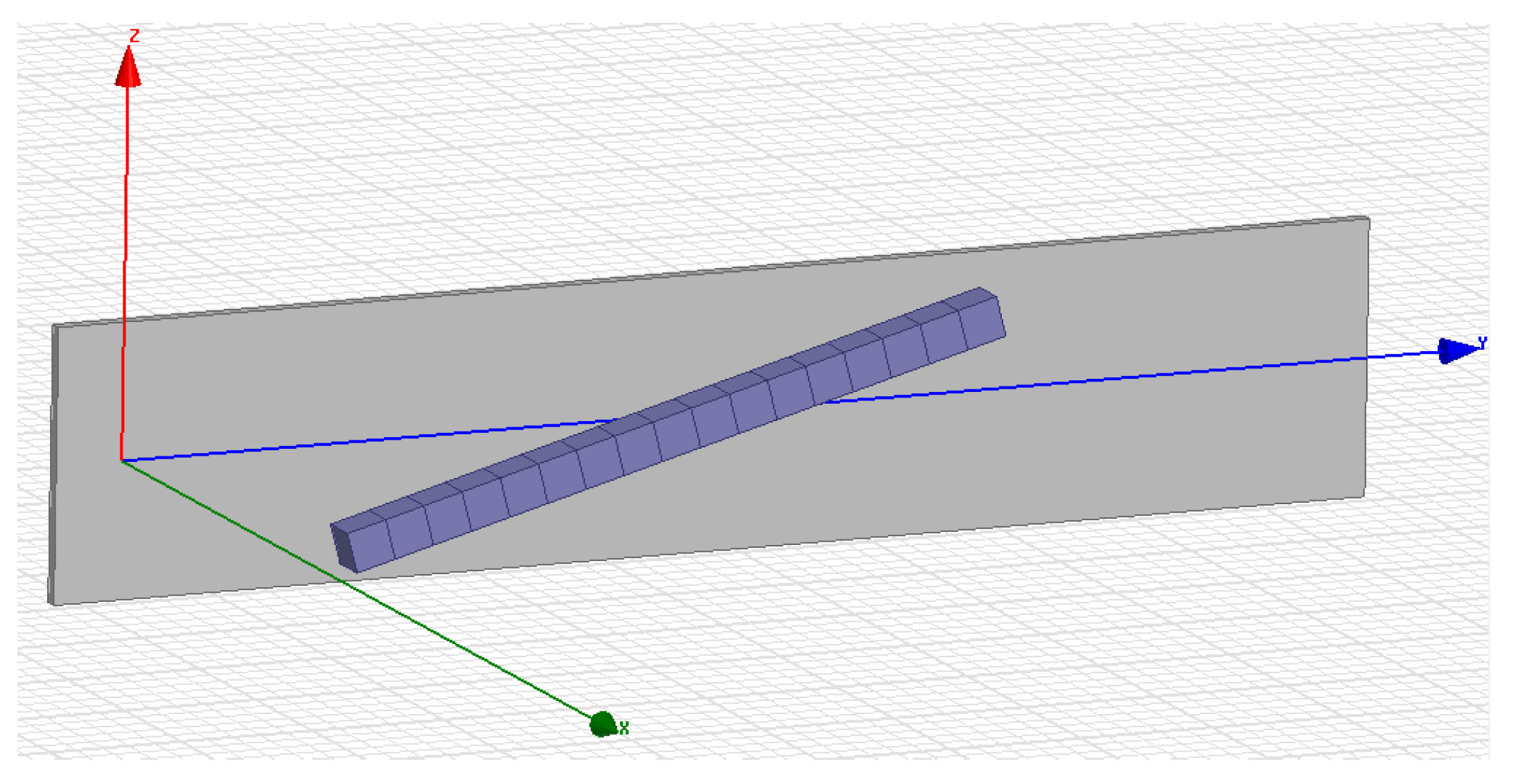
3.2. FEA Calculation

The 3-D model of the PM-EDS structure is established by using the FEA software, and the magnetic flux density and electromagnetic forces of the PM-EDS structure under various working conditions are simulated and calculated. The model parameters are shown in

Table 1. The parameters of the model.

Parameter	Value	Parameter	Value
l	0.51 m	$w_2$	0.20 m
w	0.03 m	$h_2$	0.01 m
h	0.03 m	d	0.01 m
coercivity of PM $B_r$	$1.08\times {10}^6$ A/m	$v_{\mathrm{x}}$	30 m/s
$l_2$	1 m	$\sigma$	$3.5\times {10}^7$ S/m

.

When the PM rotation angle is $\theta ={15}^{\circ }$, the 3-D simulation model and its mesh division are shown in Figure 7 and Figure 8, respectively.

3.3. Validation of Calculation Results

3.3.1. Electromagnetic Forces Validation

In a real system, the length of the conductive plate is approximately infinite compared with the PM. However, in analytical calculation and FEA calculation, it is necessary to reduce the length of the conductive plate properly to improve the calculation speed, but the error will increase if the length is set as too small. The variation in the analytical calculation result of the levitation force with the length of the conductive plate is shown in Figure 9. It can be seen that the levitation force changes very little when the length of the conductive plate is greater than 1 m, and the error is within $2\%$ compared with that when $l_2$ = 2 m. Therefore, in Table 1, the length of the conductive plate is set to 1 m after considering the calculation complexity and accuracy.

In order to verify the validity of analytical equations, the variations in levitation, drag and lateral forces with varying deflection angles are calculated by the analytical method and FEA method, respectively, and the deflection angle $\theta$ of PM ranges 0–${20}^{\circ }$. The results are shown in Figure 10. It can be seen from Figure 10 that the levitation force on the PM first increases and then decreases with the increase in the deflection angle, and the maximum value of the deflection angle $\theta$ is about ${15}^{\circ }$, which shows that it is feasible to control the levitation force by adjusting the deflection angle of the PM. Both the drag force and the lateral force tend to increase with the increase in the deflection angle. Compared with the calculation results of the analytical method and the FEA method, the relative errors are shown in Figure 11. The relative error of the levitation force is about $1\%$, and the relative error of the drag and lateral force are both within $6\%$. The results of the lift-to-drag ratio and lift-to-weight ratio are shown in Figure 12. The maximum value of the lift-to-drag ratio is $3.849$ when the deflection angle $\theta$ is $7^{\circ }$, and the maximum value of the lift-to-weight ratio is $11.30$ when the deflection angle $\theta$ is ${15}^{\circ }$.

In order to further study the characteristics of the PM-EDS system, the variations in the levitation and drag forces with varying speeds are calculated when the conductive plate is made of different materials; the results are shown in Figure 13 and Figure 14, respectively. The parameters of the model are the same as in Table 1, and the deflection angle of the PM is fixed at ${15}^{\circ }$ in order to maximize the levitation force. The conductivity of the copper plate, aluminum plate and stainless steel plate decreases in turn. The levitation forces acting on the PM all showed a tendency to increase first and then decrease with the increase in speed for different conductive plate materials, and the maximum levitation force that can be reached by various conductive plate materials is the same, while the corresponding speed when reaching the maximum levitation force is different for different materials. The smaller the material’s conductivity is, the higher the corresponding speed at the peak of the levitation force is. In the same way, the drag forces increase first and then decrease with the increase in speed, and the maximum drag force for each conductive plate material is the same. However, for the same material, the corresponding speeds are different when the levitation force and drag force reach the maximum value. For example, when the conductive plate is an aluminum plate, the levitation force reaches the maximum value at $v_{\mathrm{x}}$ = 23 m/s, while the drag force reaches the maximum value at $v_{\mathrm{x}}$ = 17 m/s.

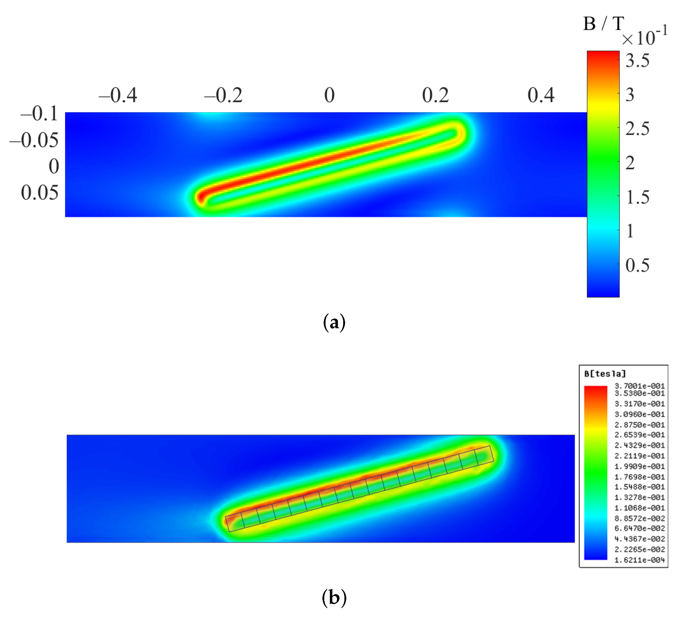
3.3.2. Magnetic Field Validation

The analysis of the magnetic flux density around the maglev train is research content that can not be ignored in the design and manufacture of a maglev train. It is necessary to evaluate the magnetic flux density of passengers, sensors and various electrical parts.

According to Equations (28)–(30), the surrounding magnetic flux density of the suspension system can be obtained by $B=\sqrt{\left({B_{\mathrm{x}}}^2+{B_{\mathrm{y}}}^2+{B_{\mathrm{z}}}^2\right)}$. Taking the upper surface of the conductive plate $y=0$ as an example, the results of the magnetic flux density on the surface calculated by theoretical method and FEA method are shown in Figure 15, where the parameters of the model are the same as Table 1, and the deflection angle of the PM is ${15}^{\circ }$. It can be seen from the comparison that the results of the analytical method and the FEA method are almost the same. The maximum value of the magnetic flux density on the upper surface of the conductive plate is about $0.37\mathrm{T}$, and the area with the strongest magnetic flux density appears in the strip-type area corresponding to the upper side of the PM. At the same time, it can be observed that due to the translational motion of the PM in the x-direction, a slight trailing effect occurs behind the tail of the PM.

4. Size Optimization of the PM

4.1. Optimization Objectives

Improving the lift-to-drag ratio and the lift-to-weight ratio is one of the most important problems in PM-EDS technology, and the size of PM has an obvious influence on the lift-to-drag ratio and lift-to-weight ratio. Therefore, the length, width and thickness of the PM are optimized by the MOPSO algorithm to maximize two competing objective functions, the lift-to-drag ratio and the lift-to-weight ratio. The objective function can be expressed as:

$$\underset{l,w,h}{\mathrm{Maximize}}\left\{\begin{array}{c}{f}_1\left(l,w,h\right)=F_{\mathrm{z}}/\phantom{F_{\mathrm{z}}{F}_{\mathrm{x}}}{F}_{\mathrm{x}}\\ f_2\left(l,w,h\right)=F_{\mathrm{z}}/\phantom{F_{\mathrm{z}}m\mathrm{g}}m\mathrm{g}\end{array}\right.$$

(37)

where function $f_1$ is the lift-to-drag ratio, function $f_2$ is the lift-to-weight ratio and $m\mathrm{g}$ is the gravity of the PM.

4.2. Multi-Objective Particle Swarm Optimization Algorithm

The MOPSO algorithm uses several particles to search in the solution space; each particle can exchange its stored information with each other and find the optimal solution according to the individual optimal value $Pbest$ and the optimal global value $Gbest$ so that the result converges to the Pareto-optimal front. Finally, a Pareto-optimal set is obtained, which contains all the nondominated solutions from the beginning to the end of the algorithm [17]. The updated equations of particles’ velocity and position of MOPSO are [18]:

$$\begin{array}{cc}\hfill & \hfill v_i\left(t+1\right)=\omega v_i\left(t\right)+c_1{r}_1\left(P_{best,i}-x_i\left(t\right)\right)+c_2{r}_2\left(G_{best}-x_i\left(t\right)\right)\hfill \end{array}$$

(38)

$$\begin{array}{cc}\hfill & \hfill x_i\left(t+1\right)=x_i\left(t\right)+v_i\left(t+1\right)\hfill \end{array}$$

(39)

where $v_i\left(t+1\right)$ and $x_i\left(t+1\right)$ are the velocity and position of the i-th particle at the $t+1$ iteration, respectively, $\omega$ is the inertia factor, $c_1$ and $c_2$ are the learning factors, $r_1$ and $r_2$ are random numbers within the range $\left[0,1\right]$, $P_{\mathrm{best},\mathrm{i}}$ is the optimal position coordinate of the i-th particle and $G_{\mathrm{best}}$ is the global optimal position coordinate.

In order to make the algorithm focus on global search at the initial stage of iterations and local search at the later stage of iterations, $\omega$ decreases with the increase in the number of iterations, $c_1$ decreases with the decrease in $\omega$, and $c_2$ increases with the decrease in $c_1$ [19]. The parameters of the MOPSO algorithm are shown in

Table 2. The parameters of the MOPSO.

Parameter	Value
Number of particles N	100
Maximum iterative number $n_{max}$	100
Inertia factor $\omega$	$0.9-0.4\left(\frac{2\left(t+1\right)}{n_{max}}-{\left(\frac{t+1}{n_{max}}\right)}^2\right)$
Learning factor $c_1$	$0.5{\omega }^2+3\omega$
Learning factor $c_2$	$4-c_1$

, where t is the current number of iterations.

4.3. Optimization Results

The length, width and thickness of the PM in the PM-EDS structure are optimized using MOPSO, and the size range of the PM is limited to: 0.01 $\mathrm{m}⩽l⩽0.8$ m, 0.01 $\mathrm{m}⩽w⩽0.3$ m, 0.01 $\mathrm{m}⩽h⩽0.3$ m. According to Figure 12, set the deflection angle $\theta =7^{\circ }$ in order to maximize the lift-to-drag ratio. According to Figure 13, we set the speed in the x-direction $v_{\mathrm{x}}$ = 30 m/s to increase the levitation force. After 100 iterations, the Pareto-optimal solutions of the lift-to-drag ratio and lift-to-weight ratio are obtained, as shown in Figure 16. Each scheme in the solution set is the optimal solution, but each scheme has a different emphasis on the two objective functions.

In Figure 16, comparing the Pareto-optimal solution set with the initial design, the lift-to-drag ratio and lift-to-weight ratio at point A are higher than the initial design; the lift-to-drag ratio at point B is higher than the initial design, while the lift-to-weight ratio is lower than the initial design. At the same time, it can be seen that the lift-to-drag ratio and the lift-to-weight ratio are two conflicting objective functions, which cannot achieve the maximum value at the same time, and the optimization of one objective will lead to the degradation of the other objective. For example, point A has the highest lift-to-weight ratio but the lowest lift-to-drag ratio with the coordinate $\left(4.71,10.07\right)$, while point B has the highest lift-to-drag ratio and lowest lift-to-weight ratio with the coordinate $\left(5.95,5.01\right)$. The selections of the length, width and thickness of the PM for each solution in the solution set are shown in Figure 17, which are the decisive factor that leads to a particular intermediate solution between points A and B.

In order to avoid the personal subjective factors in the traditional manual selection of Pareto-optimal solutions, the fuzzy set theory is used to screen the Pareto-optimal solutions, which can effectively increase the scientificity of the selection of the optimal solution. We define the membership function $S_i^j$:

$$S_i^j=\left\{\begin{array}{cc}1\hfill & ,f_i^j⩽f_i^{min}\hfill \\ \frac{f_i^{max}-f_i^j}{f_i^{max}-f_i^{min}}\hfill & ,f_i^{min}⩽f_i^j⩽f_i^{max}\hfill \\ 0\hfill & ,f_i^j⩾f_i^{max}\hfill \end{array}\right.$$

(40)

where $f_i^{max}$ and $f_i^{min}$ are the maximum and minimum values of the i-th objective function in the solution set, and $f_i^j$ and $S_i^j$ are the current value and the membership function value of the ith objective function of the j-th solution.

Next, we define the dominating function ${\phi }_k$ [20], the dominant value of the k-th solution is:

$${\phi }_k=\left\{\begin{array}{cc}{\displaystyle \sum _{i=1}^n}{S}_i^k/\phantom{S_i^k\left({\displaystyle \sum _{j=1}^M}{\displaystyle \sum _{i=1}^n}{S}_i^j\right)}\left(\sum _{j=1}^M\sum _{i=1}^n{S}_i^j\right)\hfill & ,F_{\mathrm{z}}^k⩾F_d\hfill \\ 0\hfill & ,F_{\mathrm{z}}^k<F_d\hfill \end{array}\right.$$

(41)

where M is the number of nondominated solutions. According to the optimization results, M is 63, and n is the number of objective functions, $n=2$. $F_{\mathrm{z}}^k$ is the levitation force of the k-th solution. Considering the restriction of vehicle gravity, the levitation force generated by a single PM should be greater than the expected levitation force $F_d$, and its dominant value is 0 when $F_{\mathrm{z}}^k<F_d$. Assuming $F_d=200\mathrm{N}$, the levitation force generated by each solution in the solution set is shown in Figure 18.

By substituting the Pareto solution set into Equation (41), the dominant value of each nondominated solution can be obtained. The larger the dominant value, the better the comprehensive performance of the solution. Therefore, the solution with the maximum dominant value can be selected as the optimal solution for the optimization; the dominant value of the Pareto solution set is shown in Figure 19. The dominant value of particle No. 7 is the largest, which is 0.017, and the comprehensive performance is the best. The dominant value of some particles is 0, because the generated levitation force is less than $F_d$. The corresponding parameters of particle No. 7 and particles at point A and point B and the initial design are compared in

Table 3. The comparison of parameters of particles.

Design	Lift-to-Drag Ratio	Lift-to-Weight Ratio	l (m)	w (m)	h (m)	Dominant Value
Particle No. 7	5.383	9.169	0.751	0.024	0.016	0.017
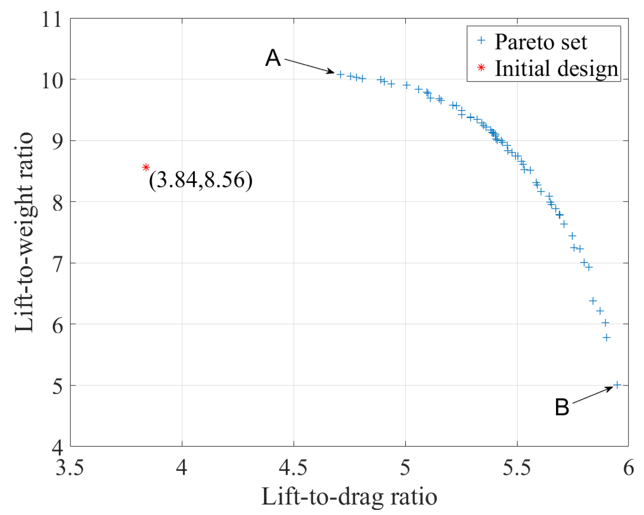
Particle at point A	4.711	10.073	0.767	0.034	0.022	0.012
Particle at point B	5.947	5.010	0.750	0.010	0.010	0.012
Initial design	3.841	8.559	0.510	0.030	0.030	-

.

It can be seen from Table 3, compared with the particles at point A and point B, that particle No. 7 has a more balanced value in lift-to-drag ratio and lift-to-weight ratio, which achieves the best trade-off for the optimal design criteria. At the same time, the lift-to-drag ratio and lift-to-weight ratio of particle No. 7 are both higher than the initial design. The size of the PM of the particle at point A is large, so it has a higher lift-to-weight ratio, but this also leads to a decrease in its lift-to-drag ratio. The length of the PM of the particle at point B is almost the same as that of particle No. 7, but the width and thickness of the PM are both the minimum values of the limited range, and the overall size of the PM is more slender, which increases its lift-to-drag ratio but decreases its lift-to-weight ratio.

5. Results

A 3-D theoretical analysis model of a PM-EDS structure with an adjustable deflection angle of the PM is established. First, by introducing SOVP, the electromagnetic forces and magnetic field of the suspension system are solved, and the variations in the electromagnetic forces of the suspension system under different deflection angles, speeds and conductor plate materials are analyzed. Secondly, an FEA simulation model is established to validate the analytical calculation results of the electromagnetic forces. The relative error of the two methods is less than $6\%$. At the same time, the results of the analytical calculation and the FEA method of the magnetic field are basically the same, which verifies the correctness of the theoretical calculation method. Finally, in order to improve the lift-to-drag ratio and the lift-to-weight ratio of the system, the length, width and thickness of the PM are optimized by using the MOPSO algorithm, and a Pareto-optimal solution set is obtained. An optimal solution is selected from the solution set by using the fuzzy set theory. The results show that the optimized lift-to-drag ratio and the lift-to-weight ratio are both higher than the initial design value. The analytical model proposed in this paper has high accuracy and an obvious optimization effect, which is of great significance to the design and research of a PM-EDS train.

References

- Guo, Z.; Li, J.; Zhou, D. Study of a null-flux coil electrodynamic suspension structure for evacuated tube transportation. Symmetry 2019, 11, 1239. [Google Scholar] [CrossRef] [Green Version]
- Montgomery, D.B. Kinematical Analysis for the Second Suspension System of the Mid-Low-Speed Maglev Vehicle. In Proceedings of the MAGLEV’2004, Shanghai, China, 26–28 October 2004. [Google Scholar]
- Fang, J.; Montgomery, D.B.; Roderick, L. A Novel MagPipe Pipeline Transportation System Using Linear Motor Drives. Proc. IEEE 2009, 97, 1848–1855. [Google Scholar] [CrossRef]
- Wang, R.; Yang, B.; Gao, H. Nonlinear Feedback Control of the Inductrack System Based on a Transient Model. J. Dyn. Syst. Meas. Control 2021, 143, 1–13. [Google Scholar] [CrossRef]
- Malewicki, D.J. Data Entry-March 31, 2052: A Retrospective of Solid-State Transportation Systems. Proc. IEEE 1999, 87, 680–687. [Google Scholar] [CrossRef]
- Malewicki, D.J. Silicon is About to Change the World-Again! Proc. IEEE 2009, 97, 1750–1753. [Google Scholar] [CrossRef]
- Fang, J.; Radovinsky, A.; Montgomery, D.B. Dynamic Modeling and Control of the Magplane Vehicle. In Proceedings of the MAGLEV’2004, Shanghai, China, 26–28 October 2004. [Google Scholar]
- Guo, Z.; Zhou, D.; Chen, Q.; Yu, P.; Li, J. Design and Analysis of a Plate Type Electrodynamic Suspension Structure for Ground High Speed Systems. Symmetry 2019, 11, 1117. [Google Scholar] [CrossRef] [Green Version]
- Bird, J.; Lipo, T.A. Modeling the 3-D Rotational and Translational Motion of a Halbach Rotor Above a Split-Sheet Guideway. IEEE Trans. Magn. 2009, 45, 3233–3242. [Google Scholar] [CrossRef]
- Theodoulidis, T.P.; Kriezis, E.E. Impedance Evaluation of Rectangular Coils for Eddy Current Testing of Planar Media. NDT E Int. 2002, 35, 407. [Google Scholar] [CrossRef]
- Musolino, A.; Rizzo, R.; Tripodi, E. Travelling Wave Multipole Field Electromagnetic Launcher: An SOVP Analytical Model. IEEE Trans. Plasma Sci. 2013, 41, 1201–1208. [Google Scholar] [CrossRef] [Green Version]
- Chen, Y.; Li, Y.; Li, Y. Three-dimensional Analytical Calculation of Plate-type Double Permanent Magnet Electrodynamic Suspension. J. Railw. Eng. Soc. 2019, 36, 29–34. [Google Scholar]
- Chen, Y. Characteristic Analysis of Electromagnetic Forces Created by Low-speed PM Electrodynamic Suspension. Ph.D. Thesis, Southwest Jiaotong University, Chengdu, China, 2015. [Google Scholar]
- Gou, X.; Yang, Y.; Zheng, X. Analytic Expression of Magnetic Field Distribution of Rectangular Permanent Magnets. Appl. Math. Mech. 2004, 3, 271–278. [Google Scholar]
- Ooi, B.T.; Eastham, A.R. Transverse Edge Effects of Sheet Guideways in Magnetic Levitation. IEEE Trans. Power Appar. Syst. 1975, 94, 72–80. [Google Scholar] [CrossRef]
- Paul, S. Three-Dimensional Steady State and Transient Eddy Current Modeling. Ph.D. Thesis, University of North Carolina at Charlotte, Charlotte, NC, USA, 2014. [Google Scholar]
- Kong, L.; Wang, J.; Zhao, P. Solving the Dynamic Weapon Target Assignment Problem by an Improved Multiobjective Particle Swarm Optimization Algorithm. Appl. Sci. 2021, 11, 9254. [Google Scholar] [CrossRef]
- Wu, C.; Li, G.; Wang, D. 3-D Analytical Modeling and Electromagnetic Force Optimization of Permanent Magnet Electrodynamic Suspension System. Trans. China Electrotech. Soc. 2021, 36, 924–934. [Google Scholar]
- Chen, G.; Wu, Y.; Gao, L.; Liu, M.; Ma, X. Optimization of Submarine Resistance Based on MOPSO. Ship Build. China 2020, 61, 392. [Google Scholar]
- Abido, M.A. Multiobjective Evolutionary Algorithms for Electric Power Dispatch Problem. IEEE Trans. Evol. Comput. 2006, 10, 315–329. [Google Scholar] [CrossRef]