1. Introduction
Neuroevolution consists of using evolutionary algorithms in training artificial neural networks. Unlike traditional, gradient-based training methods, neuroevolution can optimize the parameters of a neural network, i.e., weights and biases, and its hyperparameters, i.e., the number of hidden layers, activation functions, learning rate, etc. Neuroevolution is also suitable for both supervised and reinforcement learning applications.
In this paper, feed-forward neural networks are trained using biologically inspired optimization algorithms analyzed in previous work [
1], and we propose different strategies for combining these algorithms. According to the No Free Lunch (NFL) theorem [
2], there is no algorithm that can provide superior performance to all other techniques in solving all optimization problems [
3,
4]. Motivated by this theorem, we propose using different algorithms to learn the architecture, weights, and biases of a multilayer perceptron (MLP), in order to generate suitable regression models for the process of the free radical polymerization of methyl methacrylate (MMA).
Polymerization processes are generally notorious for the difficulty in finding suitable regression models to properly characterize them and to allow for making reliable predictions. Aside from the complexity of the underlying reactions, the phenomenology behind these processes is often not fully understood. As such, approximations of the actual phenomena have to be made when analyzing them, which adversely affects the accuracy and convergence of most conventional regression methods. Furthermore, the related mathematical models are themselves, of high complexity, which causes difficulties when solving them, requiring considerable computational resources and making them unusable in online control and optimization scenarios. Under such circumstances, empirical modeling is often the preferred approach.
In this context, MMA is among the more difficult to model chemical processes, consisting of complex reactions which cause difficulties in building a phenomenological model based on mass and energy balances. In addition to the multitude of elementary reactions and species, a volume contraction also takes place during the process. Moreover, the significant increase in viscosity from a certain moment of the reaction determines the decrease in the diffusion rate of the polymer and monomer molecules. In free radical polymerization, such diffusional aspects (gel and glass effects) must be quantified by relations which should render the variation of the propagation and termination rate constants with the conversion. This is a difficult part to model, especially because not all the aspects of these phenomena have been completely explained.
In order to overcome the difficulties related to the modeling of the controlled diffusion phenomena, neural networks prove to be suitable tools for modeling, provided that they are developed in a near-optimal version for both structure and parameters.
The optimization goal is to find MLPs with the best prediction performance, i.e., the minimization of prediction error, on the MMA data set (conversion and molecular masses depending on reaction conditions). The optimization algorithms we use are the Football Game Algorithm (FGA) [
5], Imperialist Competitive Algorithm (ICA) [
6], Simple Human Learning Optimization (SHLO) [
7], Social Learning Optimization (SLO) [
8], Teaching-Learning-Based Optimization (TLBO) [
9], Viral System (VS) [
10], and Virulence Optimization Algorithm (VOA) [
11].
The main contribution of the paper is finding a neural network optimizer that generates optimal neural network-based regression models for a proper representation of the MMA process. Our studies show that conventional regression models fail to properly achieve this task. Consequently, we propose a multi-step process that ultimately analyses and tests several optimization algorithms and combines them into ensembles of optimizers using three proposed strategies: hybrid cascade, hybrid single elite solution, and hybrid multiple elite solutions. We also use an initial search procedure to determine the best parameter values for each algorithm considered in this paper. Based on the result provided by the search procedure, we identify the three best-performing algorithms and use them in each proposed ensemble strategy. Each individual algorithm is run for a longer period, while the algorithms in an ensemble are run for a significantly shorter time. For each simulation scenario, we collect performance statistics at specific iterations to perform a fair comparison between strong individual optimizers and the proposed ensembles of weak optimizers. As we demonstrate in
Section 4, the most suitable model for our problem results from a combination of three biologically inspired optimizers using the hybrid multiple elite solutions strategy. To our knowledge, this is the first instance when multiple biologically inspired optimization algorithms have been combined in such a manner, for the study of complex chemical processes such as MMA.
The paper is structured as follows:
Section 2 presents a brief review of some of the more notable results from the related literature; in
Section 3 we provide a detailed description of our method: the dataset containing the experimental values pertaining to our problem, the encoding approach for transforming the neural network parameters into a format usable by an optimization algorithm, as well as the strategies for tuning, selecting and combining several algorithms into ensembles;
Section 4 presents our experimental results, where we compare the best-performing algorithms with their various ensemble arrangements so as to find the approach that provides the best regression models for our problem; the paper ends with a Conclusions Section where we discuss our contribution and findings and point out the main directions for future work.
2. Related Work
In recent years, neuroevolution has received particular attention, and numerous works present successful applications in different fields, such as chemistry [
12,
13,
14], medicine [
15,
16,
17], and games [
18,
19]. However, one cannot identify a single evolutionary optimization technique that generally leads to the best results. Therefore, various algorithms for training neural networks are proposed in the literature [
20,
21,
22,
23,
24,
25]. For example, in [
26], a new implementation for the Clonal Selection Algorithm (CSA) is proposed, which is used in training MLP neural networks. To significantly increase the classification accuracy of MLPs, CSA is used to find the optimal weights and biases. The proposed approach is compared with other training methods on five data sets, and the obtained results show that the new approach is a competitive method for training MLPs. A new learning strategy based on neuroevolution for designing and training optical neural networks (ONNs) is proposed in [
27]. The authors use Genetic Algorithms (GA) and Particle Swarm Optimization (PSO) algorithms to determine the hyperparameters of ONNs and optimize the connection weights. Experimental results show that the proposed strategy is competitive with traditional learning algorithms such as Stochastic Gradient Descent (SGD) and Adjoint Variable Method (AVM). In [
28], the problem of remaining useful life (RUL) prediction using Spiking Neural P (SN P) systems is addressed. The authors use the Neuro-Evolution of Augmenting Topologies (NEAT) algorithm to optimize the structure and parameters of SN P systems. The results show that the proposed approach provides a reasonable trade-off between performance and the number of trainable parameters. Additionally, in [
29], the Moth–Flame Optimization (MFO) algorithm is used to train MLP networks. An autonomous navigation robot data set is used, and MFO is used as an optimizer to find the optimal weights and biases. The obtained results show the exploration and exploitation capabilities of MFO in comparison with other methods.
However, in the context of a prediction problem, it is known that ensemble-based approaches tend to have better accuracy, efficiency, and flexibility than approaches using a single classifier [
30]. Due to these advantages, the use of ensembles has been addressed in the field of evolutionary algorithms.
A new neuroevolutionary model with quantum inspiration, called NEVE (Neuroevolutionary Ensemble), is proposed in [
31] and is based on an ensemble of MLP neural networks to learn in nonstationary environments (when data distribution changes over time). Each neural network in NEVE is trained and has its parameters optimized by the quantum-inspired evolutionary algorithm with binary-real representation (QIEA-BR). The authors propose four variations of the NEVE algorithm that are evaluated on both real and synthetic data. The obtained results confirm that the neuroevolutionary ensemble approach is a suitable choice for those problems whose data sets are subject to sudden changes in behavior.
The idea of multiple subpopulations and bagging ensemble is used in [
32] to generate new offspring in the multi-objective differential evolution (MODE) algorithm. In the proposed BagMPMODE algorithm, each subpopulation is regarded as a bootstrapped population, and the evolution process of each subpopulation is regarded as a base learner. The idea of cooperation between subpopulations is introduced by randomly sampling a solution from each subpopulation and generating new offspring. Depending on the quality of each subpopulation, specific weights are determined and used in the offspring generation procedure. A randomly selected parent from a better subpopulation has a larger contribution to the genes of the new offspring. Finally, the generated offspring replaces the weakest solution from a randomly selected subpopulation. The authors compare the efficiency of the BagMPMODE algorithm with the version of the algorithm where the bagging-based search is not adopted (MPMODE). Experimental results show that BagMPMODE significantly improves the search efficiency on 20 out of 22 multi-optimization problems compared to MPMODE.
The ensemble learning (EL) based on Adaboost is adopted in [
33] for a dynamic multi-objective optimization evolutionary algorithm (DMOEA). Multiple base models are used to predict new populations using a shared population, and the weight associated with each base model is determined based on the prediction error. A strong model is defined based on the weights determined as follows: a base model that has a higher weight has a higher chance of being incorporated into the strong model. At the end of an iteration, the strong model generates a new, improved population used in the next iteration. The proposed EL-DMOEA algorithm combines different strategies and benefits from an improved convergence.
In [
34] are proposed different strategies for hybridizing a Genetic Algorithm (GA) with a Genetic Programming (GP) algorithm. The population of GP is regarded as a pool of base classifiers (i.e., arithmetic trees) that are improved during the GP search. However, at different iterations of GP, the authors choose to sample the current population of GP to create multiple subpopulations of a given size. Each subpopulation in GP is regarded as an ensemble of base classifiers and is coded as a single chromosome in GA. The GA search procedure aims to find an ensemble with the best combination of base classifiers. Experimental results show that the proposed hybridization approach and its different strategies provide ensembles of classifiers that significantly outperform the standard GP. It is also interesting that the authors observe degraded performance when ensembles contain a larger number of classifiers (greater than seven), possibly due to increased ensemble complexity.
Four individual niching genetic algorithms are used in [
35] to form an ensemble. The authors choose two instantiations of the restricted tournament selection (RTS) and two of the clearing (CLR) algorithms as niching algorithms. The basic principle is to use four parallel populations, where a particular niching algorithm owns a population. Although a specific algorithm handles a population, a collaborative strategy between populations is achieved using a shared pool of newly created offspring from each niching algorithm. The parallel populations are iteratively evolved until a maximum number of function evaluations is reached. Experimental results show that the proposed ensemble scheme locates more optima than any of the individual niching algorithms in most cases.
In [
36], an approach that adapts evolution strategies for evolving an ensemble model is presented. A subset of sensor data represents the input data of each model in the ensemble, and neuroevolution is used to optimize the architecture and hyperparameters of each model. Other studies can also show the advantages of using ensemble learning with evolutionary computation [
37,
38,
39].
3. Materials and Methods
Our approach consists in a multi-step process that involves the analysis, tuning, selection, and combination of multiple biologically inspired optimization algorithms. The overall method is depicted in
Figure 1. The chemical process considered in this paper is influenced by three inputs. The experimental data are processed within a pipeline involving the following steps:
Analysis of several popular algorithms in terms of their usefulness. This involves a hyperparameter search in order to find the best versions of the algorithms (i.e., the parameter values which result in the lowest RMSE);
Selection of the best algorithms, out of previously tested ones. Out of all algorithms, only the top few are further used;
Incorporation of the selected algorithms into various hybrid ensemble strategies, the purpose being to find the strategy which ultimately leads to optimal neural network architecture, with the potential to provide meaningful predictions for the three outputs of our studied process.
3.1. Data Set
The polymerization process is approached by modeling the conversion and numerical and gravimetrical average molecular masses (three outputs) depending on the reaction conditions: time, initiator concentration, and temperature (three inputs). The data set consists of 3217 samples split into 75% for training and 25% for testing.
Other methodologies have also been tested on this process by our research group. The first series of attempts [
40,
41] implied the design of neural networks of feedforward type, with satisfactory results for conversion, but not acceptable for molecular weights. A more complex approach, which led to better results [
42] was based on combining a simplified phenomenological model with neural networks, obtaining hybrid models. Several modeling modalities were considered, namely the neural networks have replaced different parts of the model—in general, the parts are difficult to model due to diffusion-controlled phenomena (gel and glass effects). The results obtained were much better than the models represented by single neural networks, but also not very satisfactory for gravimetrical molecular weight. Another attempt [
43] was based on different regression methods: Large Margin Nearest Neighbor Regression algorithm trained either with an evolutionary algorithm or by gradient descent and Nearest Neighbor Regression with Adaptive Distance Metrics Trained by Multiple Point Hill Climbing on Noisy Training Set Error. Acceptable results were obtained with these methods, but there is still room for improvement.
The main goal of the present approach is to test a series of algorithms, combined with different optimization strategies, for obtaining a near-optimal artificial neural network, thus developing an efficient methodology that can be easily and successfully adapted to other processes (models). MMA polymerization, a real complex process, is a choice suitable for the proposed purpose representing a difficult test for the optimization algorithms.
3.2. Neural Network Modeling
This section describes the use of biologically inspired optimization algorithms for training MLP neural networks. An MLP neural network architecture consists of an input layer, an output layer, and one or more hidden layers, and each of these layers contains a certain number of neurons. Adjacent layers of the MLP are fully connected, and each connection between two neurons has an associated weight. The values of weights and biases are adjusted in a supervised manner using an optimization algorithm. Since we are normalizing the data set in the range [−0.9, 0.9], we choose the hyperbolic tangent activation function (1) for each neuron:
We use the notation [ni-nh1- … -no] to describe the architecture of an MLP, where ni represents the number of neurons in the input layer, nh1 represents the number of neurons in the first hidden layer (the number of neurons of this layer is illustrated in bold), and no represents the number of neurons in the output layer. For example, the notation [7-5-2] describes an MLP with seven inputs, five neurons in the hidden layer, and two outputs.
In this paper, we use different algorithms to optimize the architecture, weights, and biases of MLP neural networks to obtain networks with the best prediction performance on the MMA data set. A population-based algorithm uses a set of candidate solutions (i.e., individuals) that evolve through an iterative process. Individuals in the population are created or modified using different operators specific to the algorithm. In our case, a solution represents a neural network, and a population is equivalent to a set of neural networks. An individual’s objective function is evaluated using the root mean square error (RMSE) (2) of the MLP on the training or testing data set. Therefore, minimizing the RMSE value is the primary goal of the algorithm:
where
ns is the number of samples in the training or testing data set,
no is the number of outputs of the MLP,
dij is the desired MLP
jth output at
ith training or testing sample, and
yij is the actual MLP
jth output at
ith training or testing sample.
A coding and decoding step is required in training MLP neural networks with such algorithms. The coding step consists of extracting information from an MLP structure and organizing it into a specific representation compatible with a candidate solution used by an algorithm. In this paper, we code the solution as a fixed-length one-dimensional array of real values. A general case of an MLP structure and its associated coded solution is illustrated in
Figure 2.
The locations in the solution array illustrated in
Figure 2 are described as follows:
nl: the number of hidden layers of the neural network. This number can be different from one network to another and is an integer value in the range [nlmin, nlmax];
nh1: the number of neurons in the first hidden layer. nh1 is an integer value in the range [nh1min, nh1max];
nh2: the number of neurons in the second hidden layer. nh2 is an integer value in the range [nh2min, nh2max]. This location is only used when nl = 2;
wi-h1: the weight values associated with the connections between the neurons of the input layer (i) and the neurons of the first hidden layer (h1). These locations always exist in the solution array because all networks we use have at least one hidden layer;
wh1-h2: the weight values associated with the connections between the neurons of the first hidden layer (h1) and the neurons of the second hidden layer (h2). These locations are only used when nl = 2;
wh2-o: the weight values associated with the connections between the neurons of the second hidden layer (h2) and the neurons of the output layer (o). These locations are always used in the solution array. If the second hidden layer does not exist (nl = 1), then these locations represent the weights associated with the connections between the neurons of the first hidden layer (h1) and the neurons of the output layer (o);
bh1, bh2, bo: the biases of neurons in each layer. The locations for bh2 are only used when nl = 2.
The MMA data set we use has three inputs (ni = 3) and three outputs (no = 3). Therefore, we define certain limits on the number of neurons in each layer of the neural network as follows:
nl ∈ [
nlmin = 1,
nlmax = 2]: neural networks always have at least one hidden layer and at most two hidden layers. These limits are recommended in [
44];
nh1 ∈ [
nh1
min = 7,
nh1
max = 12]: in the first hidden layer, the neural networks can have a minimum of seven and a maximum of twelve neurons. These limits are recommended in [
45] as
nh1
min = 2 ⋅
ni + 1 and
nh1
max =
no ⋅ (
ni + 1);
nh2 ∈ [
nh2
min = 2,
nh2
max = 4]: in the second hidden layer, neural networks can have a minimum of two and a maximum of four neurons. These limits are recommended in [
45] as
nh1
min = 3 ⋅
nh2
min and
nh1
max = 3 ⋅
nh2
max (i.e., the number of neurons in the second hidden layer is three times smaller than the number of neurons in the first hidden layer);
The values of weights and biases are real values in the range [−3, 3].
Limiting the number of neurons in each layer of the neural network implies limiting the search space of the algorithms. Depending on the defined limits and the characteristics of the data set, the maximum length of the solution array is determined using the Equation (3), where the value 3 represents the locations assigned to the structural information (i.e.,
nl,
nh1,
nh2),
nwmax and
nbmax represents the maximum number of locations assigned for the weights and biases,
ni in the Equation (4) represents the number of input features, and
no in the Equations (4), (5) represents the number of output features specific to the data set:
The limits chosen for each location of the solution array are constant throughout the simulations. The operators of the algorithms can change the value of any location in the array. However, these changes are limited by the predefined range of each location.
Since the coding has a fixed-length representation, there may be unused locations for some neural network structures. For example, consider the case of MLPs with one input (
ni = 1), one hidden layer (
nl = 1), at most four neurons in the hidden layer (
nh1
max = 4), and one output (
no = 1). Based on these bounds, the MLPs [1-
4-1] and [1-
2-1] are associated with an array of the same length (
Figure 3). One can see in
Figure 3 that MLP [1-
2-1] contains unused locations (grey colored) for some weights and biases. A particular case can occur when two solutions must be combined. Since the algorithms do not check for invalid or unused locations, the combination of two individuals can unintentionally behave as a mutation operator when the value of a used location (i.e., meaningful data) is combined with the value of an unused location (i.e., noise).
3.3. Strategies for Combining Optimization Algorithms
In the following, different strategies are proposed for combining the algorithms in an ensemble of optimizers. We use the original implementation of each optimizer except the TLBO algorithm. In general, we observed long simulation times in the case of TLBO and introduced a slight change in the algorithm to minimize the number of interactions between individuals. More specifically, in the teacher phase of TLBO, we allow the teacher to interact with only 30% of random students (instead of all students), and we apply the same constraint in the learner phase.
In the proposed ensembles of optimizers, we use some basic procedures that handle a single solution or a set of solutions. Although these procedures may vary from one strategy to another, their basic principles are described as follows:
Solution fetching procedure: one or more solutions are fetched from an algorithm that has reached its termination criterion;
The procedure for applying the mutation operator: some genes of one or more fetched solutions are modified;
Solution transfer procedure: a set of solutions (i.e., population) is provided as the initial population to an algorithm. In this procedure, we ensure that the population provided to the algorithm has a size compatible with the algorithm configuration.
The procedures described involve minimal changes to the existing implementation of the algorithms in [
1]. Specifically, each algorithm is adapted to accept an input population as the initial population. The input population size must be compatible with the algorithm configuration. If no population of individuals is provided at the input of the algorithm, then the initial population is created according to the procedure in the algorithm (i.e., a population of randomly generated individuals).
Regarding the ensemble models in this paper, we use only the three best-performing algorithms in all the proposed strategies. Our reasoning is to eliminate those less efficient algorithms for the given problem to maximize the performance of an ensemble. We believe this is a good approach because the most suitable algorithms will be used depending on the given optimization problem.
Moreover, we propose to use a minimal number of iterations for any algorithm used in an ensemble. This approach is based on the popular idea of an ensemble of weak learners [
46]. In our case, a weak learner is correlated with a weak optimizer, the generation of a data subset is correlated with the generation of a population, and the combined responses of the weak learners are correlated with an improved population containing the best solutions from the weak optimizers. The main focus is to use an ensemble of weak optimizers and compare the performance of the ensemble with the performance of strong individual optimizers. The motivation of this approach is that an ensemble of weak optimizers could lead to better convergence.
3.3.1. Choosing the Best Performing Algorithms
The step of choosing the algorithms with the best performance consists of a search procedure for the best parameter values for each of the implemented algorithms (FGA, ICA, SHLO, SLO, TLBO, VS, and VOA). This step is performed only once, and the best parameter values found are used in all subsequent runs.
The search procedure randomly generates nconf sets of values for the algorithm parameters. We choose a predefined range of values for each parameter in a single algorithm. Based on each parameter’s predefined range of values, we randomly generate a set of parameter values for the chosen algorithm. However, we keep only that set for which the algorithm provides the solution with the best objective function value. Since the algorithms are based on random events, it is expected that the same set of parameter values will provide slightly different solutions. Therefore, we perform several runs (nruns) for a single set of parameter values to obtain average results.
After determining the three best-performing algorithms, we use them in various ensemble strategies described in the following sections.
3.3.2. Hybrid Cascade Strategy
In the hybrid cascade strategy (
Figure 4), we propose that a single solution be sequentially transferred from one algorithm to another. The initial solution is randomly generated and then used to generate a population of
N individuals (population_1). We choose
N to have the same value as the
population size parameter of the first algorithm in the sequence (Algorithm_1). In this strategy, the procedure to generate a population is suggestively called
GeneratePopulation_1-to-N to reflect that we are using a single individual in generating a population of
N individuals. In the first step of this procedure, we perform a simple cloning operation of the initial solution
N times. In the last step, we apply a mutation operator to each cloned solution, thus obtaining a population of modified individuals. The mutation operator we use is identical for all proposed ensemble strategies, and we describe it in the Mutation Operator section. However, it is worth mentioning that applying the mutation operator to the entire population can lead to the loss of the global best solution. Therefore, we always use elitism, i.e., the best individual is copied directly into the next population provided by the
GeneratePopulation_1-to-N procedure. Elitism applies to any
GeneratePopulation procedure used in other ensemble strategies.
The first population generated is provided to the first algorithm, which is run with a minimal number of iterations. At the end of the run, we take the best solution from the first algorithm and use it to generate a new population for the second algorithm. This sequence continues until the best solution is obtained from the last algorithm used in the hybrid cascade strategy. A complete run of this sequence is correlated with a single ensemble iteration. The desired number of ensemble iterations (ensemble_iter) is performed by repeatedly running the described sequence and transferring the best solution from one ensemble iteration to the next.
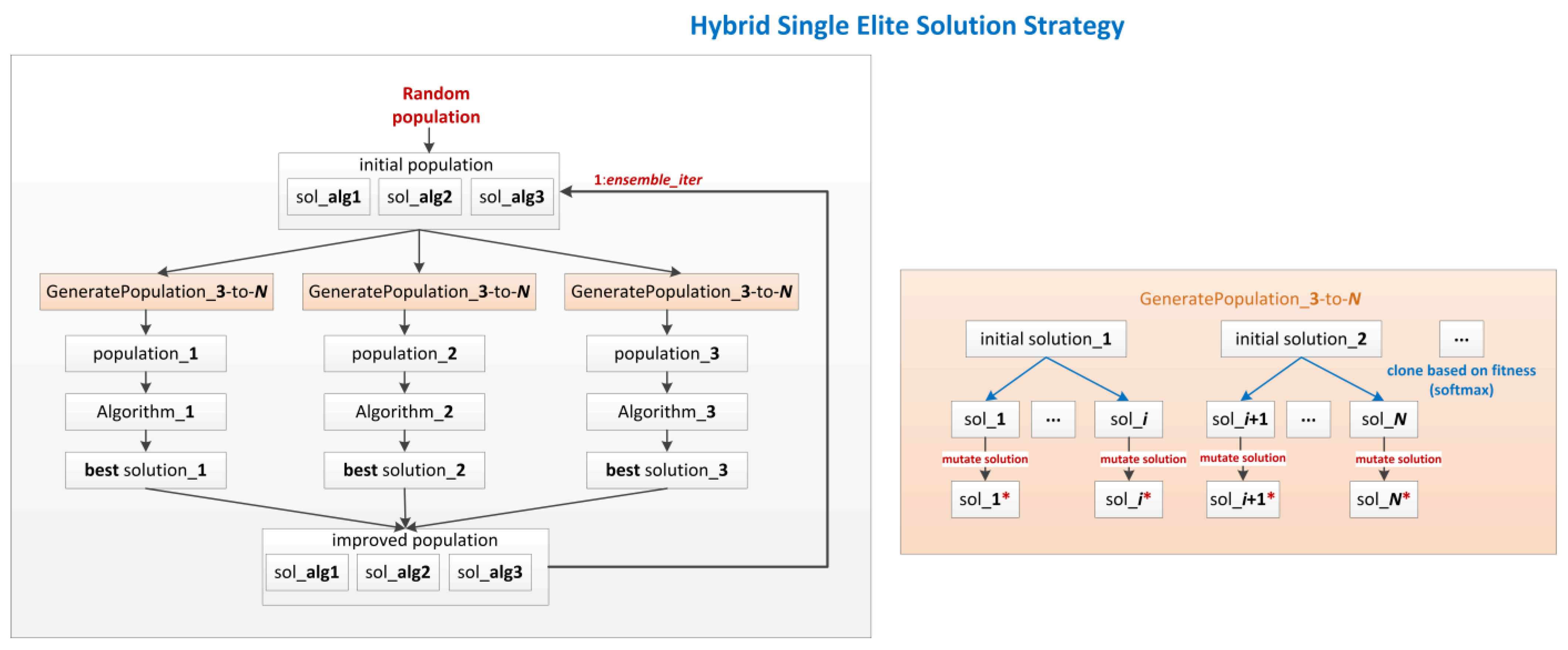
3.3.3. Hybrid Single Elite Solution Strategy
In the hybrid single elite solution strategy (
Figure 5), we propose that an algorithm does not depend on the results of other algorithms at the same ensemble iteration. However, at the end of an ensemble iteration, we take the best solution from each algorithm in the ensemble to define an improved population. Thus, a new ensemble iteration will use the previous improved population as the initial population. The suggestive name of the “single elite solution” strategy is derived from the fact that we take only one solution (i.e., the elite) from each algorithm to define an improved population.
In the hybrid single elite solution strategy, an ensemble iteration always starts from a population of three individuals. Therefore, the population generation procedure is suggestively called
GeneratePopulation_3-to-N. If a different number of algorithms are used in the ensemble, e.g.,
NoAlg ≥ 2, the population generation procedure is adapted for the general use case, i.e.,
GeneratePopulation_NoAlg-to-N. In this procedure, we propose that the cloning operation of the initial solutions is influenced by their objective function value. Let the initial solutions be
s1,
s2, …,
sn and their objective function values
f1,
f2, …,
fn. We use the objective function values
f1,
f2, …,
fn to determine the weights
w1,
w2, …,
wn associated with the initial solutions using the softmax function:
Since the goal is to minimize the RMSE value of an MLP, in (6) we use the objective function value with a negative sign to obtain higher weights for solutions with a lower objective function value. The obtained weights determine the number of cloning operations for each initial solution. In other words, we clone a larger number of fitter solutions and a smaller number of less fitted solutions. For example, if the initial solutions s1, s2, s3 have the objective function values f1 = 0.01, f2 = 0.5, f3 = 0.9, then their weights are approximatively w1 = 0.5, w2 = 0.3, w3 = 0.2. Therefore, for a population size of N = 100 individuals, a population of 50 s1 clones, 30 s2 clones, and 20 s3 clones will be generated.
In the last step of the GeneratePopulation_NoAlg-to-N procedure, we apply the mutation operator to each cloned solution to obtain the final population.
One can see in
Figure 5 that the population generation procedure is used independently for each algorithm. The main reason we generate different populations is that each algorithm requires a population of a different size. Additionally, generating different populations leads to better diversity that could improve ensemble performance.
3.3.4. Hybrid Multiple Elite Solution Strategy
The third proposed ensemble strategy is similar to the hybrid single elite solution strategy, but the population generation procedure differs. In the hybrid multiple elite solution strategy (
Figure 6), we use a larger initial population, and the population generation procedure is based on the bagging technique [
47]. More precisely, in the procedure called
GeneratePopulation_Bagging, we randomly sample
N solutions from the initial population (sampling with replacement). The obtained intermediate population (i.e., bootstrapped population) is then modified by mutating each individual to obtain the final population.
In this paper, we use an ensemble of three algorithms. After the termination criterion of the algorithms is reached at the end of an ensemble iteration, the improved population is created based on the performance of each algorithm. We propose that the improved population contains 15% elites from the best algorithm, 10% elites from the second best algorithm, and 5% elites from the worst algorithm. Since each algorithm has a specific population size, the size of the improved population may vary when the algorithms are sorted according to their performance in a new order (i.e., the algorithms may perform differently on new iterations). Similar to the previous strategy, the improved population in the current ensemble iteration becomes the initial population in the next iteration.
3.3.5. Mutation Operator
The mutation operator in all population generation procedures consists of modifying individuals’ genes using a Gaussian random number. The mutation we use has a certain chance of altering an individual’s genes, thereby improving the diversity of the population. The mutation operator proposed in this paper is described in the following Algorithm 1:
| Algorithm 1 The mutation operator. |
Mutate-individual inputs: x: the individual’s genes mutProb: the individual’s chance to be mutated mutGain: control factor for genes mutation chance : variance outputs: x*: the resulted individual ---------------------------------------------------------------------------------- // check if the individual should be mutated or not if mutProb < rand() then x* x // no mutation performed else // check which genes should be mutated geneMutProb foreach gene in x if geneMutProb > rand() then x*[gene] x[gene] + Gaussian(gene,) return x*
|
The terms used in Pseudocode 1 are described as follows:
mutProb represents the probability that the mutation operator is applied to the given individual;
mutGain represents a factor that controls the mutation probability of each gene;
Gaussian(gene,) is a Gaussian random number with a mean equal to the gene value and variance ;
rand() is a uniformly distributed random number in the range [0, 1).
The parameter values we use in the mutation operator are mutProb = 0.5, mutGain = 2 and = 1.
4. Experiments and Results
In this section, we present the experiments performed and evaluate the MLP training efficiency of strong individual optimizers and ensembles of weak optimizers. Performance evaluation is completed using the root mean square error (RMSE) on the training and testing samples data set. We determine the RMSE at specific iterations to obtain a convergence curve graph during the optimization process.
Our original implementation for MLP allows us to access parameter information from the neural network easily. The C# implementation of the algorithms from paper [
1] is used, and for the scope of this paper, we extend this implementation to training MLPs with these algorithms. We also implement the three ensemble strategies proposed in this work: hybrid cascade, hybrid single elite solution, and hybrid multiple elite solutions.
The experimental simulations are performed on machines with different specifications, and the execution time cannot be fairly evaluated. For this reason, we consider the number of evaluations as an index of the processing power used for a given individual optimizer or ensemble of optimizers. An evaluation counter is incremented each time an optimizer uses the objective function. We observed that the objective function is the most time-consuming procedure, with ~98% processing time, which is similar to the timing profile of NEAT [
48]. In this function, a solution array is decoded into an MLP structure, and then the RMSE of the MLP outputs is calculated using the training or testing samples.
The data set consists of 3217 samples split into 75% (2412) training samples and 25% (805) testing samples.
Our experimental setup consists of two main steps, as illustrated in
Figure 7. In the first step, we randomly search the parameter values for each algorithm. The search procedure is used to identify the three best-performing algorithms, and the best parameters found for these algorithms will be used in all subsequent simulations. We choose a fixed number of 300 iterations for each algorithm, while the other parameters can vary. The configuration of the search procedure is
nconf = 50 random sets of parameter values for each algorithm and
nruns = 2 independent runs to average the results. Since the search procedure is time-consuming, we do not use a larger number for
nruns.
The parameter limits for an algorithm are appropriately chosen to avoid inconsistent combinations of parameter values. For example, in the ICA algorithm,
no. empires must not exceed
pop. size, but the chosen limits do not allow such an inconsistent combination to be generated during the search procedure.
Table A1,
Table A2,
Table A3,
Table A4,
Table A5,
Table A6 and
Table A7 in the
Appendix A show the limits we choose for each parameter of an algorithm and the results of the search procedure: the best parameter values, the average RMSE calculated on the training samples, the average number of evaluations, and the structure of the best neural networks.
Based on
Table A1,
Table A2,
Table A3,
Table A4,
Table A5,
Table A6 and
Table A7, we show in
Table 1 the algorithms sorted (from best to worst) according to their performance using the RMSE value averaged over
nruns = 2 runs. One can see that the first three best-performing candidates are ICA, TLBO and SHLO. Although the algorithms presented in
Table 1 show a different number of evaluations, in the present paper we do not investigate the causes that lead to these obtained values (e.g., parameter settings or early stopping conditions). It is not the purpose of this work to present a detailed comparison between the individual algorithms. Therefore, we choose three algorithms for which we obtain the lowest mean RMSE value (using the settings presented in
Table A1,
Table A2,
Table A3,
Table A4,
Table A5,
Table A6 and
Table A7) and compare their individual performance with the ensembles created with the same algorithms.
In the second step of our experiments, we choose ICA, TLBO, and SHLO as the base optimizers. In
Figure 7, we illustrate that we perform six main simulations. In the first three simulations, each algorithm is run using 300 iterations. Since this is a large number of iterations, we correlate an algorithm with this configuration with a strong individual optimizer. The other three simulations represent the run of each proposed ensemble strategy. A base optimizer is run with five iterations in a single ensemble iteration, and we correlate it with a weak optimizer. Therefore, a single ensemble iteration is equivalent to 15 cumulative iterations from three weak optimizers. We choose 20 ensemble iterations for each ensemble strategy to obtain a cumulative number of 300 iterations (i.e., the same number of iterations as a strong individual optimizer). Our reasoning is to perform a fair comparison between strong individual optimizers and ensembles of weak optimizers. We run all six simulations with thirty independent runs to obtain statistically meaningful results.
Figure 8 shows the convergence curve graphs of all six simulations obtained on the training and test samples. The curve graphs of the individual optimizers ICA, TLBO, and SHLO are shown with continuous lines, while the curve graphs of the ensemble strategies are shown with dashed lines. We illustrate on the
x-axis the current number of an ensemble iteration. In the case of individual optimizers, one ensemble iteration is equivalent to fifteen individual iterations. Therefore, we collect performance statistics from individual optimizers every 15 iterations. On the
y-axis, we show the RMSE obtained at each ensemble iteration (i.e., at every 15 iterations of the individual ICA, TLBO, and SHLO algorithms) averaged over 30 independent runs.
We can see in
Figure 8 that the convergence curve graphs for the training and test samples are very similar in shape but have different scales. During the first ten ensemble iterations, all three ensemble strategies outperformed the individual optimizers in convergence speed. It is interesting to note that hybrid cascade ensemble has better convergence than hybrid single elite solution. However, these ensembles have similar performances after the 10th ensemble iteration. The best overall performance is observed for the hybrid multiple elite solutions ensemble, outperforming all individual algorithms and the other two ensemble strategies. A hybrid multiple elite solutions ensemble is an extension of hybrid single elite solution because it uses a larger population of elites. Therefore, we argue that the increased performance of the hybrid multiple elite solutions ensemble comes from creating a more diverse improved population at the end of each ensemble iteration.
The individual ICA optimizer has a slow convergence, but after 300 iterations, it achieves a performance similar to that of the hybrid multiple elite solutions ensemble (at ensemble iteration 20). However, for some problems, 300 iterations might be a large value, and choosing the multiple elite hybrid solution strategy is preferred.
In
Table 2, we present the detailed simulation results for the individual ICA, TLBO, and SHLO optimizers at iteration 300 and the results of the proposed ensemble strategies at ensemble iteration 20. We can see that the hybrid multiple elite solutions ensemble provides the smallest errors with a mean RMSE train of 0.00582 and a mean RMSE test of 0.01029. The same ensemble provides the best solutions with an RMSE train of 0.00517 and an RMSE test of 0.00932. The number of evaluations of the hybrid multiple elite solutions ensemble (39,245) is competitive with the number of evaluations of the individual optimizers ICA (37,159), TLBO (40,424), and SHLO (40,033). Therefore, the faster convergence and smaller errors provided by the hybrid multiple elite solutions ensemble make this strategy the preferred choice.
We can see in
Table 2 that each ensemble strategy has roughly the same number of evaluations, i.e., 39,200. This is an expected result because we use the same configuration of weak optimizers in all ensemble strategies. However, we emphasize that the value of 39,200 is the approximate average of the number of evaluations from the individual optimizers ICA (37,159), TLBO (40,424), and SHLO (40,033). Since we use an equal number of iterations (i.e., five) for each weak optimizer in all ensemble strategies, each ensemble inherits the average computational effort of the individual optimizers. However, choosing an unbalanced number of iterations for weak optimizers of an ensemble is an easy way to control the trade-off between inherited computational effort and inherited performance. To investigate the impact of an unbalanced number of iterations for weak optimizers, we present in
Figure 9 the convergence curve graphs of each ensemble strategy for the following scenarios:
Scenario 1: five iterations are used for each weak optimizer in all ensemble strategies. This is the original experiment setup, and we use it as a baseline comparison. The convergence curve graphs for this scenario are shown in
Figure 9 with continuous lines and are labeled Cascade-balanced, SingleElite-balanced, and MultipleElite-balanced;
Scenario 2: nine iterations for ICA weak optimizer and three iterations for TLBO and SHLO are used. In this scenario, we want the ensembles to inherit, to a greater extent, the characteristics of the best optimizer, i.e., ICA. The convergence curve graphs for this scenario are shown in
Figure 9 with dashed red lines and are labeled Cascade-ICA, SingleElite-ICA, and MultipleElite-ICA;
Scenario 3: nine iterations for TLBO weak optimizer and three iterations for ICA and SHLO are used. In this scenario, we want the ensembles to inherit, to a greater extent, the characteristics of the second best optimizer, i.e., TLBO. The convergence curve graphs for this scenario are shown in
Figure 9 with dashed blue lines and are labeled Cascade-TLBO, SingleElite-TLBO, and MultipleElite-TLBO;
Scenario 4: nine iterations for SHLO weak optimizer and three iterations for ICA and TLBO are used. In this scenario, we want the ensembles to inherit, to a greater extent, the characteristics of the worst optimizer, i.e., SHLO. The convergence curve graphs for this scenario are shown in
Figure 9 with dashed gray lines and are labeled Cascade-SHLO, SingleElite-SHLO, and MultipleElite-SHLO.
Note that we use a cumulative number of 15 iterations for the weak optimizers in all scenarios. We choose this number of iterations for convenience because the results for
Scenario 1 are already available, and new simulations are unnecessary. We also show in
Figure 9 only the convergence curve graphs on train samples because the curve graphs on test samples are very similar in shape but have different scales.
We can see in
Figure 9a,b that the Cascade-ICA and SingleElite-ICA ensembles inherit slower convergence from the ICA individual optimizer. The Cascade-TLBO and SingleElite-TLBO ensembles inherit faster convergence from the TLBO individual optimizer, but the Cascade-SHLO and SingleElite-SHLO ensembles show no promising improvement. Therefore, we can say that Cascade and SingleElite ensembles are sensitive to an unbalanced number of iterations for weak optimizers.
On the other hand, we can see in
Figure 9c that the MultipleElite-ICA ensemble has a better convergence in the first seven ensemble iterations compared to the balanced ensemble, which is not an intuitive outcome. In the case of the MultipleElite-TLBO and MultipleElite-SHLO ensembles, we observe slightly poorer performance in the first seven ensemble iterations. However, we can see that the MultipleElite ensemble is stable because MultipleElite-ICA, MultipleElite-TLBO, and MultipleElite-SHLO perform similarly to MultipleElite-balanced after ensemble iteration 7. The performance stability of the MultipleElite ensemble provides the advantage of using an unbalanced number of iterations. In other words, in the MultipleElite ensemble, we can favor the weak optimizer with less computational effort without losing ensemble performance. We show in
Table 3 the performance of each ensemble in the four scenarios (at ensemble iteration 20).
Based on the results in
Table 3, we can see that the MultipleElite ensemble performs similarly for balanced and unbalanced number of iterations for weak optimizers. Additionally, the MultipleElite-ICA ensemble inherits a lower computational effort (i.e., 38,261) from the individual optimizer ICA (37,159). The presented results demonstrate that our proposed hybrid multiple elite solutions ensemble is a simple and promising ensemble strategy that benefits from the best performance of the base optimizers in terms of accuracy and computational effort.
5. Conclusions
In this paper, we addressed the concept of neuroevolution, where the algorithms FGA, ICA, SHLO, SLO, TLBO, vs., and VOA were used to find the architecture, weights, and biases of neural networks. Using a search procedure, we identified three best-performing algorithms and combined them using three proposed ensemble strategies: hybrid cascade, hybrid single elite solution, and hybrid multiple elite solutions. The proposed ensemble strategies are easy to implement because they do not involve changes in the logic of the algorithms. Instead, the proposed strategies involve simple methods of generating populations and transferring them to the algorithms.
We used the MMA dataset to train neural networks with variable structures using each individual algorithm and the proposed ensembles constructed with the same algorithms. The training performance of individual optimizers was compared with that of the ensemble of optimizers, and we observed that hybrid multiple elite solutions outperformed all optimizers in convergence speed. We believe this performance is due to a more diverse population that we create at each iteration of the hybrid multiple elite solutions ensemble. Using a larger number of iterations, one of the individual optimizers, i.e., ICA, achieves a prediction accuracy similar to that of the ensemble. However, ICA has a very slow convergence. Furthermore, we have analyzed the effect of using an unbalanced computational effort for weak optimizers, and the experimental results demonstrate that a hybrid multiple elite solutions ensemble is a stable strategy. Our experimental results show that the hybrid multiple elite solutions ensemble is the strategy that generates neural network-based regression models that provide the best representation of the underlying process behind MMA, and which have the potential to generate the most dependable related predictions. Furthermore, given that there is no precise phenomenological model for this process, the predictions provided by the optimal neural network prove to be of real use in industrial practice, successfully replacing a series of experiments that consume time, materials, and energy. In addition, the proposed model can be easily introduced in an online control procedure for optimal control. Additionally, to our knowledge, such a neural network optimization strategy has not been used before for such a process, while performing better than other well-established biologically inspired optimizers.
A future research direction is to evaluate the performance of the proposed ensembles of optimizers on a larger number of optimization problems. The proposed ensemble strategies can be seen as adaptive optimizers that combine the characteristics of individual optimizers. Therefore, we believe this approach would provide competitive results because an ensemble is always constructed with a subset of optimizers performing better on a given optimization problem.


