MSSA: Constant Time State Search through Multi-Scope State Area

Abstract

In the stateful data plane, the switch can record the state and forward packets based on the local state. This approach makes it possible to integrate complex network applications into the data plane, thus reducing the amount of communication required between the switch and the controller. However, due to the time it takes to look up the state for packets, packet-forwarding latency has increased. With increased network traffic, a large number of states may be recorded in the switch, and the problem of increased packet-forwarding latency caused by the lookup state becomes more serious. In this paper, we propose the multi-scope state area (MSSA) for recording state inside the switch, which can achieve a fixed-time state lookup in a large-scale state. MSSA divides the state sharing scope by associating with the switch’s multiple match–action tables, and the shared scope is used to determine the state area for recording state. When processing a packet, the state required will only be in a limited number of states that are recorded in a few state areas. We implemented a prototype pipeline that supports MSSA based on Intel’s DPDK framework and investigated the effect of state type, number, location, and comparison method on state search/insertion time. The results show that the cost of MSSA search state is constant, regardless of the number of states, and MSSA has a high space utilization rate.

1. Introduction

Software-defined networking (SDN) decouples the network’s control plane and data plane, bringing unprecedented programmability to the network and encouraging the development of network algorithms. Many network algorithms (such as congestion control [1,2,3,4], scheduling [5], measurement [6,7,8], active queue management [9,10,11,12,13], security [14], and load balancing [15,16,17,18]) require the creation and modification of algorithm-defined states during packet traversal through the switch in order to respond to network emergencies [19]. However, in a traditional SDN, a centralized controller manages network states, while the stateless data plane is only responsible for packet forwarding and lacks state-processing capability. As a result, the states of these network algorithms can only be recorded in the control plane and processed by the controller [20]. The remote-control delay and communication overhead between the switch and the controller do not just reduce the response speed of network applications; they also increase the controller’s burden and impact the controller’s decision-making quality [21].

A lot of work has been proposed to maintain states in the data plane to enhance the response time of network applications and reduce the controller’s burden [22,23]. OpenState [24], the early stateful data-plane proposal, proposed the use of an extended finite state machine (XFSM) to improve the data-plane programmability, and the XFSM function was supported in the follow-up work, Open Packet Processor [25]. FAST (flow-level state transition) [26] uses state machine filter tables to isolate the states of different applications and speed up state search, while SDPA (Stateful Data Plane Architecture) [27] uses Forwarding Processors (FP). FlowBlaze [28] introduces an extended finite state machine (EFSM) [29] to maintain flow states and global states inside the switch, enhancing state-programming capabilities. The widely used network programming scheme P4 [30] supports the use of metadata to store a temporary state between flow tables and global registers for the persistent recording state.

Although processing the state in the data plane improves network programmability, the time overhead added by looking up the state when processing packets may seriously harm switch’s performance, which is exacerbated when there are a large number of states inside the switch [31]. Even though a data structure such as a cuckoo hash table [32] can guarantee constant lookup time, it may require a non-constant insertion time [28]. Slow insertion will also have a negative impact on the switch’s throughput. For example, when performing 60 updates per second, the OpenFlow switch’s throughput will be reduced by two times [33]. Furthermore, the network device’s storage space is limited, and ensuring the state search speed may necessitate sacrificing the device’s storage space. In a load-balancing application, for example, tens of millions of connections are tracked at the same time, and storing the states of 10 million connections in a match–action table requires hundreds of MB of SRAM, whereas the available SRAM in the latest generation of switches is only 50–100 MB [17].

In this paper, to ensure constant-time state search and insertion, as well as to optimize storage space utilization, we propose a state storage structure named multi-scope state area (MSSA) and a corresponding state search algorithm. By using MSSA, it is possible to achieve the following: (1) constant-time state search and state insertion; (2) effective use of state storage space and timely recovery of useless space. More precisely, the multi-scope state area is a hierarchical tree structure for storing states that is connected to the switch’s multilevel match–action table structure. MSSA can limit the state search scope and possible insertion position in packet forwarding by utilizing the inherent operation of the match–action table. Therefore, constant-time state search and insertion are possible due to the limited size of the state area and the number of states stored in it. Because MSSA is associated with the match–action table structure, the state area can be allocated or released by following the addition and deletion of table/entries, the useless state area can be released in time, and the state storage space can be fully reused.

In summary, we make the following contributions:

• We propose the multi-scope state area (MSSA) that stores state in a hierarchical tree structure. MSSA is associated with the switch’s multilevel match–action table structure to split the scope of state sharing packets and reuse state storage space in time. Based on the scope of state sharing, we categorize the state into four types, namely global state, table state, flow state, and packet state, and stores them in different state areas.
• In the MSSA, we also propose the state search and state programming methods. The state search method, according to the state-sharing scope, reduces the state required in packet processing to a limited range, enabling constant-time state search. State programming is accomplished by reusing the switch’s existing functions (match–action table and instructions), thus reducing expansion costs and improving compatibility.
• We built a packet forwarding pipeline that supports MSSA. Moreover, in the MSSA’s state search/insertion time, we evaluated two state-comparison methods and state store-space utilization.

The rest of the paper is organized as follows. In Section 2, we introduce the match–action model, which is the most widely used packet processing model in data-plane forwarding devices. Then, we introduce the MSSA’s structure, as well as the state search and state programming methods that fall under this structure. In Section 4, we depict the implementation of the packet forwarding pipeline that supports MSSA, as well as the results of the state search/insertion time, two state-comparison methods, and MSSA space utilization. In Section 5, we introduce related work, and we conclude in Section 6.

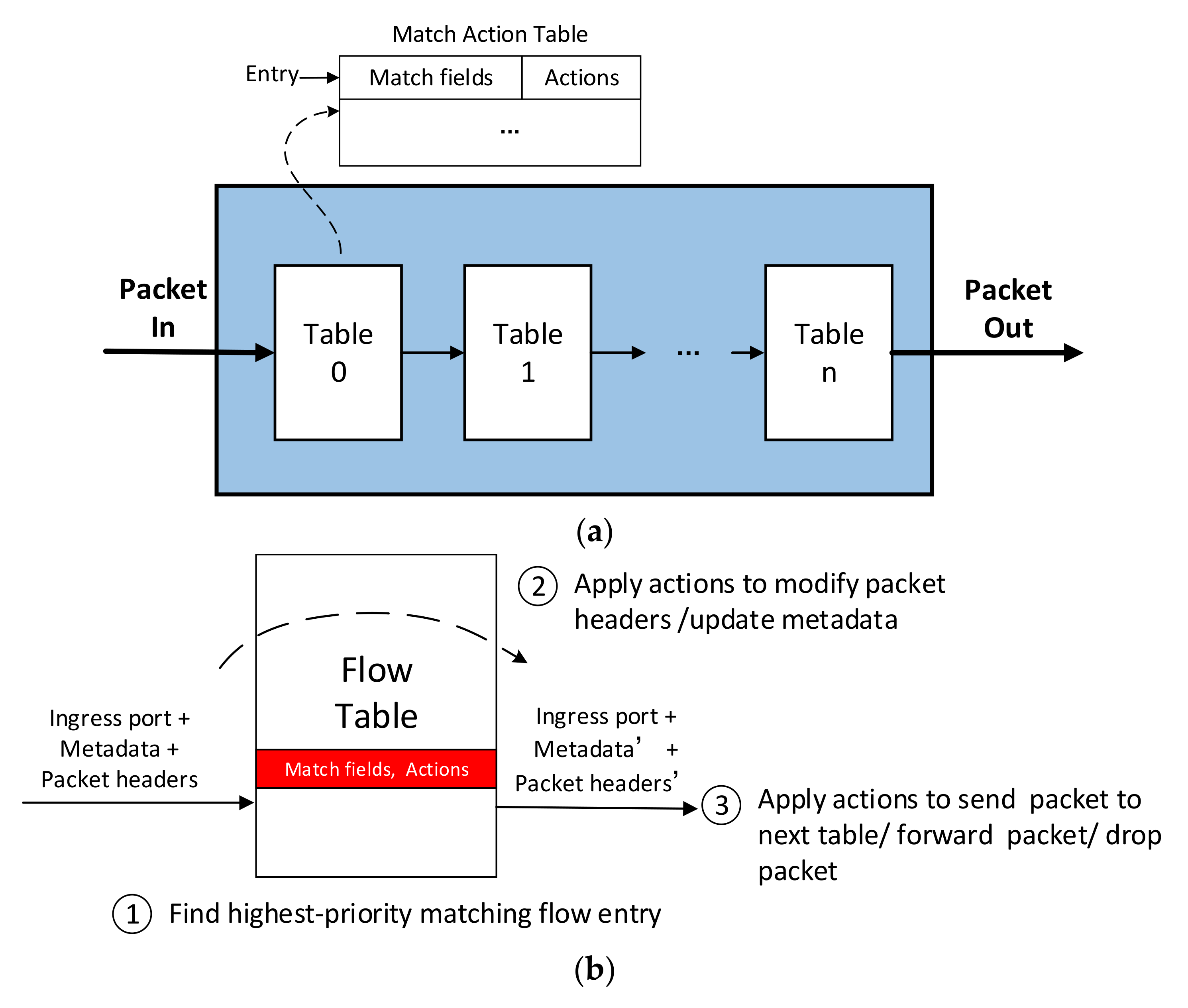
2. Match–Action Model

The match–action model is the most widely used model for data-plane programmable devices to process packets. This is primarily due to its abstraction of “flow”, that is, the set of traffic defined by the wildcard rule on the packet’s header field. Additionally, the flow abstraction makes it possible for the programmer to effectively implement L2/L3 forwarding, firewall, and QoS logic familiar to the processing logic in the traditional data-plane device [34]. The match–action model is widely used in data-plane programming languages (OpenFlow1.1+ [35], P4 [30]), reconfigurable ASICs (RMT [36]), software switches (OVS [37], Eswitch [38]), and programmable core data paths (eBPF/XDP [39]) (FastClick [40], BESS [41], NetBricks [42]).

To describe the packet processing logic, the match–action model uses a series of tables containing user-defined two-tuples (rules–actions) [43]. As shown in Figure 1, the switch’s pipeline processes packets through one or more match–action tables (MAT). The pipeline always starts with the first MAT to match packets. Table entries include packet match fields and packet processing actions. A packet is processed if an entry in the MAT matches it, and the action in that entry can direct the packet to another MAT to continue matching. If not, the packet is processed by the table’s default entry. Normally, the default entry will either send the packet to the controller or discard it.

Extract the matching field to match the MAT and get the highest priority matching entry, where the matching field can come from the packet’s ingress port, packet header fields, or metadata. (2) The action in the matching table entry may modify the packet or metadata. (3) The action in the matching table entry will send the packet to other flow tables, forward the packet to the port, or discard the packet [35]. As can be seen, the match–action model focuses on packet field processing and lacks state processing capabilities. Even though metadata can be used to store user-defined states, the data in metadata are only available for a limited time. As soon as the packet leaves the pipeline, the state data are lost [44].

To understand the difficulty of processing state on the data plane, we first introduce the concept of state [22]. The network defines state as the data that should be stored in the network device to process future packets. For example, a stateful firewall tracks the connection state and decides whether to allow or reject a packet based on that state. Reference [23] summarizes the three key features of the stateful data plane: (1) the state can be saved in the data plane, (2) the data plane can update its own saved state, and (3) the data plane is programmable.

It is not easy to satisfy all three characteristics on the data plane while also acting as the state to help the switch process future packets. The problem is as follows:

(1)

The state storage structure affects storage space utilization and search speed.

As previously stated, using the match–action table to record the states of tens of millions of connections requires far more space than the switch’s SRAM can provide. Using the match–action table to record states is a bit wasteful. As shown in

Table 1. Record states in the match–action table.

Flow Key	State
IPsrc = … …	OPEN
IPsrc = 1.2.3.4	STAGE-1
IPsrc = 5.6.7.8	STAGE-2
IPsrc = no match	DEFAULT

, the table must record the state, as well as the matching key used to get it. These keys may already exist in other tables, and storing them multiple times wastes space. Furthermore, all states are stored in a single table, likely to result in state explosion and a slow search speed [31].

(2)

Multi-flow state sharing.

We now know that the state helps the switch in packet processing. If the state-recording packet and the state-using packet do not belong to the same flow, that is, if a state is shared by two or more flows, storing this state in a single table becomes difficult, because these flows may not have the same field value as the key used to identify the state.

OpenState [24] proposes lookup and update scope methods, that is, a state is associated with two fields, and the two flows can find the state through different fields. This method fails when there are more than two flows sharing the state and it is not scalable. Global registers were introduced by OPP [25] and Flowblaze [28] to solve multi-flow state sharing issues. The recorded state is obtained by different flows via the register’s name, while, in large-scale scenarios, the limited number of global registers and storage space makes this inefficient.

(3)

State programming.

The match–action model has matured with the development of SDN and is now widely used in data-plane programming languages and devices. As a new direction, the stateful data plane is still being developed. Adding dedicated modules for state programming or designing new state programming languages face enormous implementation and compatibility challenges.

In summary, this paper proposes a multi-scope state area structure to meet the needs of storage, update, and programmability of the state on the data plane, as well as a way to improve state space utilization while reducing state search time overhead.

3. Multi-Scope State Area (MSSA)

3.1. MSSA Structure

MSSA is a state-storage hierarchical tree structure. The MSSA structure has four layers, as shown in Figure 2, namely the global state area, the table state area, the flow state area, and the packet state area, where the state area is a sub-unit that records the state. In order to classify state areas, each state is assigned a specific sharing scope, and all of the states in the same state area have the same sharing scope.

The state-sharing scope refers to the set of packets that are allowed to share the same state in a switch. We divided four packet scopes in the switch by using the multilevel match–action table: all packets in the switch, packets entering the same match–action table, packets matching the same entry, and a single packet. The state is divided into four types based on these four packet scopes.

Global state (gs). Packets entering different tables share it. As shown in Figure 3a, the global state, $S_0$, is shared by packets entering the $T_0$ or $T_2$ tables.

Table state (ts). Packets entering the same table share it. As shown in Figure 3b, the states $S_1$, $S_2$, and $S_5$ are shared by all packets entering the $T_0$ table, they are $T_0$’s table state. Similarly, T1’s table state is $S_3$, $S_4$.

Flow state (fs). Packets matching the same entry share it. As shown in Figure 3c, $S_5$ is only used by packets matching entry $R_0$, so $S_5$ is further divided into entry $R_0$ flow state. Similarly, $S_2$ is the flow state of the $R_2$ entry.

Packet state (ps). Shared by a single packet. As illustrated in Figure 3d, the state $S_6$ is only shared by the packet P, which is used to transfer information between different flow tables.

The global state, table state, and flow state are all saved in their respective areas (global state area, table state area, and flow state area), as is the packet state in the packet state area. Although there are only four types of states, there are more than four state areas. Consider the table state in Figure 3b. $S_1$ and $S_3$ are both table states, but $S_1$ is shared by packets entering table $T_0$ and $S_3$ is shared by packets entering table $T_1$. Their sharing scopes differ, and they must be placed in different state areas.

As shown in Figure 4, we associate MSSA with the switch’s multilevel match–action tables to clearly define the state’s shared scope. In the switch, each table has a table state field, each table entry has a flow state area, and each packet has a packet state area. The switch maintains one global state area. Then, at time T, the total number of state areas in the switch is shown in Equation (1).

$${\mathrm{sa}}_{\mathrm{T}}=1+t+{\displaystyle \sum }_{i=0}^t{f}_i+{\displaystyle \sum }_{i=0}^p{P}_i$$

(1)

In detail, at time T, 1 represents the number of global state areas, t represents the number of tables in the switch, ${{\displaystyle \sum }}_{i=0}^t{f}_i$ represents the total number of entries in the switch, and ${{\displaystyle \sum }}_{i=0}^p{P}_i$ represents the total number of packets received by each switch port.

State access will be restricted after dividing it by sharing scope. The state cannot be accessed when the packet is not within its shared scope. As shown in Figure 3c, the state $S_2$ is only accessible when the packet matches the entry $R_2$. Similarly, the state in the $T_0$ table state area can only be accessed by packets entering the $T_0$ table, the state in the packet state area can only be accessed by its associated packet, and the state in the global state area can be accessed by all packets entering the switch.

The following are the advantages of using MSSA:

(1)

Fine-grained division states.

The state is fine-grained divided into state areas based on shared packet scope. If a state is only used by one flow, it can be stored in the flow state area associated with the matching flow entry. Moreover the number of states in a flow state area is significantly less than the total number of states in the switch, and this makes sense. Even for stateful applications that require the storage of multi-flow sharing states (such as MAC learning and stateful firewalls), a majority of shared-state flows are bidirectional. Two-way flow will enter the same table, allowing the shared state to be recorded in the table state area. MSSA can fine-grainedly divide a large number of switch states into various tables, entries, and packet state areas. The state-sharing scope limitation can narrow the search range and avoid the long search or insertion times that occur when the state is stored in the one big table. The state’s storage location is close to the use state’s packet, allowing for faster state querying.

(2)

Any kind of state sharing.

MSSA is able to meet any state sharing needs, despite the sharing scope’s restrictions on state access in the state area. The state shared by packets from different flows can be placed in the nearest common parent node of the packet state area in MSSA’s tree structure.

At time t, packet a matches Table 1 entry 1, packets b and c match Table 1 entry i, and packet d matches table t entry j, as shown in Figure 5. Because both c and d will match Table 1 entry i, the shared state of them must be placed in the Table 1 entry i’s flow state area. Meanwhile, packets a and d enter different tables, so the state shared by both of them need to be placed in the global state area.

Although the sharing scope limits state access, the packet in the switch can share the state with any other packet. In the worst-case scenario, the state is recorded in the global state area. While a large number of table state areas and flow state areas can relieve the pressure on the global state area.

(3)

Rapid state space recovery and reuse

It is difficult to determine whether a state shared by multiple flows can be deleted, even if some of the flows have left the switch. Because the state recorded on the data plane is not backed up, an accidental deletion of the state will not only affect the logic of the network application, but it will also be irreversible. As a result, using a table to record the status and setting a timeout period for the states is risky.

MSSA is linked to the match–action table, and the state area with a shared scope can specify the state’s deletion time. When an entry is deleted, the state in the flow state area associated with the entry can be deleted as well. Because the flow-state area’s state is only shared by packets that match the entry. There will be no more packets matching the entry after the entry is deleted, so the related state can be safely deleted. Similarly, the state in the table’s associated state area can be deleted after the table is deleted. Therefore, MSSA not only allows for fine-grained state division and narrows the scope of state search, but it also allows for the safe and timely deletion of states, freeing up storage space for the continued storage of new states.

In summary,

Table 2. Four types of states’ sharing scope, life cycle, and quantity in the switch.

Type	Sharing Scope	Life Cycle	Amount
Global state	all packets in the switch	= Switch	1
Table state	packets entering the table	= Table	Number of tables
Flow state	packets matching the entry	= Entry	Number of entries
Packet state	a single packet	= Packet	Number of packets

summarizes the four types of states’ sharing scope, life cycle, and amount.

3.2. State Lookup

Although the switch has $1+t+{{\displaystyle \sum }}_{i=0}^t{f}_i+{{\displaystyle \sum }}_{i=0}^p{P}_i$ state areas at time T, the packet processing state can only be in four state areas at most. Because the number of states that can be stored in each state area is limited, constant-time state lookup is possible. By the shared scope of the state, there can be only four state areas needed in packet processing. When a packet matches an entry, it can only access the following state areas: the packet’s packet state area, the matching entry’s flow state area, the entering table’s table state area, and the global state area (as shown in Figure 6). The state required by the packet will then be limited to these four states. Obviously, the limited state areas can only be determined after the packet matches the entry. As stated in Section 2, the switch processes packets by using a match–action table. Moreover, matching the packet to an entry is a switch-inherent process.

Assume that each state area has a maximum storage capacity of M states. If there are no restrictions on the state sharing scope, even if the state is divided into multiple state areas, in order to obtain a state, we must first locate the state area, and then obtain the state. The time complexity of locating the state area in this case is shown in Equation (2).

$$\mathrm{O}(1+t+{\displaystyle \sum }_{i=0}^t{f}_i+{\displaystyle \sum }_{i=0}^p{P}_i)$$

(2)

However, due to the state sharing scope limitation, the state required by the packet can only be in four state areas, so the time complexity of looking up the state area is O(1), which is a constant. There are at least M states in the state area, and even if linear search is used, one of the states can be obtained in constant time. As a result, using MSSA, a state can be found in real time.

When processing a packet, Algorithm 1 describes the process of looking up the state. The state is identified by type and name, where type denotes the type of state (packet state, flow state, table state, and global state), and name uniquely identifies the state within the state area. When the packet enters the switch, the global state area, gsa, and the packet state area, psa, can be determined. When the packet matches an entry, the table’s state area, tsa, and the matching entry’s flow state area, fsa, can be determined. As a result, in the state lookup, first get the state area based on the type of state (lines 1, 3, 5, and 7) and then look up the state value based on the state name (lines 2, 4, 6, and 8).

Algorithm 1. Look up the state

Input: state s = {type,name}, global state areas gsa, packet enters table’s state area tsa, packet matches entry’s flow state area fsa, packet state area psa Output: state value 1. If $\mathrm{s}.\mathrm{type}$ == packet state: 2.           Find the state value according to $\mathrm{s}.\mathrm{name}$ in $\mathrm{psa}$ 3. If s. type == flow state: 4.            Find the state value according to s.name in fsa 5. If s. type == table state: 6.            Find the state value according to s.name in tsa 7. If s. type == global state: 8.            Find the state value according to s.name in gsa 9. Return state value

In summary, MSSA restricts the scope of state sharing; the states that packets can find or store in packet processing are limited to four state areas. Therefore, constant-time state search and insertion can be realized when the number of states stored in each state area is limited.

3.3. State Programming

The ability of a switch to expose packet processing logic and allow the control plane to systematically, quickly, and completely reconfigure it is referred to as programmability. Unlike traditional fixed-function network devices, which allow only a limited number of forwarding strategies to be changed (for example, adding static IP routes or changing ACLs), the programmable switch offers a forwarding table that matches any header field and atomic actions for packet processing [43]. In the data plane, state programming is based on such ability. Moreover, the programmable switch can save the state, update the state, and change the packet processing decision based on the local state [23].

MSSA does not require the addition of new types of tables or actions, instead relying on the programmable switch’s existing functions (match–action tables, arithmetic and logic operations, comparison jumps instructions, etc. [36]) to support state programming. We use the method proposed in the article [45] for supporting multiple types of data processing on the data plane, using {type, offset, length} to represent packet fields and different types of states. The data type is indicated by the type. We used five data types in this paper: packet, packet state, flow state, table state, and global state; offset indicates the offset of the data relative to the starting position. For example, the offset of the packet field is relative to the offset of the header’s starting position, and the offset of the state is relative to the offset of the state area in which it is located. Moreover, length indicates the length of the data. By reusing the match–action table and instructions in the switch, state storage, update, and state-based packet processing can be realized.

3.3.1. State Storage and Update

However, even though the “type, offset, length” representing the state does not specify the state area, the type can be used to determine the state area, because, after matching the entry, the packet can access up to four state areas, each of which is of a different type. Moreover, offset and length can also be used to determine the state’s position within the state area. Once the location of the state has been determined, the switch’s assignment instructions can be reused to store or update the state in a specific location.

It is worth noting that when the state is a matching field, it can only be in one of three state areas, as shown in Figure 7. Because the packet has not yet matched an entry, we cannot get the state of the matching entry’s flow state area in advance. As a result, the state can only be in the global state, table state, or packet state areas when used as a matching field. When the state is used as an instruction parameter, it can be in one of four states because the packet has already matched the entry.

This method necessitates network applications that manually plan the state area’s space. Although it is unfriendly to programmers, each state area can only store a limited number of states. Directly specifying the location can reduce the time overhead of finding the state within the state area even further. In the future, we will improve the friendliness of programmers and shield the low-level details of state locations by using network programming languages.

3.3.2. State-Based Packet Processing

Realizing state-based packet processing necessitates the following steps: get state, compare state value, choose packet processing decision based on comparison result, and update state. According to the preceding content, the state can be obtained by using {type, offset, length}, indicating the position of the state, and the state can be stored or updated by the switch’s assignment instruction. Furthermore, there are two ways to compare the state value: (1) use the state as a matching field and (2) compare the state value by using the compare jump instruction.

The match–action table, as shown in Figure 8a, contains two matching fields: the packet destination IPv4 address and the global state $s_1$. When the state $s_1$ is 1, perform the operation of updating $s_1$ to 2 and forwarding the packet from port 0; when the state $s_1$ is 2, perform the operation of updating $s_1$ to 3 and forwarding the packet from port 1. This method implements state programming with simple logic and stable performance, but it takes up too much entry space when the number of states to be compared is large.

Figure 8b performs the same function as Figure 8a’s match–action table. Figure 8b, on the other hand, compares the state by using the compare jump instruction. The table’s matching field only contains the packet’s destination IPv4 address, and the entry compares the state and branches based on the state value. This method avoids taking up extra entry space due to state comparison. However, there is a limit to the number of executable instructions in the switch’s pipeline. Exercising too many instructions will result in an increase in time overhead. We compared and tested the two state comparison methods in terms of space occupied and impact on forwarding performance in our experiment.

4. Implementation and Evaluation

4.1. Implementation

To focus on verifying the constant-time state search under the MSSA structure proposed in this article, we independently implement the packet forwarding pipeline used to verify the method in this paper, as shown in Figure 9. The pipeline implements the match–action table function by using the EM table lookup algorithm in the librte_table library provided by DPDK, and expands the table and entry structure to associate the corresponding table state area and flow state area. When the pipeline creates the table, the table state area and the flow state area are reserved according to the declaration. Furthermore, the pipeline uses the headroom in the DPDK’s packet structure Mbuf as the packet state area. When Pipeline is first started, it creates a global state.

Before processing the packet, the pipeline will obtain five addresses: packet header’s base address, packet state area’s base address, flow state area’ base address of the packet matching entry, table state area’s base address of the packet entering table, and the global state area’s base address. These are useful for obtaining the packet field or state based on {type, offset, length} later on.

Each type of state area is configured with a fixed size in the pipeline implementation. The greater the scope of packets shared by the state area, the more states that could be stored. As a result, we allocated 1 M bytes to the global state area, 1 K bytes to the table state area, 16 bytes to the entry state area, and 8 bytes to the packet state area.

To process packets and state, the pipeline employs a set of atomic actions (

Table 3. Pipeline actions.

Category	Actions
Arithmetic logic	add, sub, srl, sll, and, or, xor, nor, not, set, insert, del, calculate_checksum
Forwarding	goto_table, output, flood
Branch	jump, compare_jump

). Arithmetic logic actions (and, or, not, assignment, etc.), forwarding actions (jump table, output, and flooding), and branch actions are all included (jump and compare jump).

4.2. Evaluation

We tested the performance of the MSSA proposed in this paper in two directions: the time it takes to find/insert the state and the amount of space consumed by the storage state.

Table 4. System-under-test data sheet.

CPU	Intel Xeon CPU E7-4809 v4 @2.10 GHz
Caches	32 k L1 i and L1 d, 256 KB L2, 20 MB L3
Memory	128 G DDR3 @ 1333 MHz, 4-channels
NIC	Intel XL710, PCI Express 3.0/x8, 4*10 Gb Intel I350, PCI Express 3.0/x8, 4*1 Gb
DPDK	v19.11

shows the experimental platform that was used to run the Pipeline in the experiment. To generate test packets, the experiment employs the Sprient Testcenter C50.

4.2.1. State Search and Insertion Time

We proposed that MSSA be used to store the state and that the state be expressed with type, offset, and length. This experiment investigates the effects of state number, type, offset, and length on state search/insert time.

(1)

Number of states

The purpose of this experiment is to see how the number of states stored in the switch affects state search and insertion time. The global state area in the experiment stored 10, 100, 1000, 10,000, 100,000, and 1,000,000 states, each with a length of 1 byte. In the experiment, packet matching entries used the following actions: (1) OUTPUT(s), where the OUTPUT action must find the state s = {gs, 0, 8} and forward the packet based on the state value; and (2) SET(s, 1), OUTPUT(0), where the SET action inserts a state s = {gs, 0, 8} and the OUTPUT action forwards the packet to port 0.

The experimental results show that, regardless of the number of stored states, the forwarding latency of a packet is 13.78 us when searching or inserting a state during the packet processing, indicating that the number of stored states has no effect on the state search/insertion time. Because the {type, offset, length} that represent the state are relative to the state’s pointer. Obviously, the number of states stored in the switch has no effect on the time it takes the pointer to read and write data. Because all states are stored in the global state area in this experiment, they are all global states. In Experiment (2), we examined the effect of state type on the time required to search for/insert a state.

(2)

Type of state

In this experiment, we used Sprient Testcenter C50 to generate 10 Gbps, 64 bytes, and 5 different IPv4 destination flows, each matching 5 entries. All of these entries use the SET (s, 0), OUTPUT (s) action processing packet. The offset (0) and length (8 bits) of state s are the same in different entries, but the types are different, namely packet header field, packet state, flow state, table state, and global state.

Figure 10 depicts the experimental results. The type of state has no effect on the time it takes to search for or insert a state, and the time it takes to search for or insert a state is constant. The reason for this is that, prior to executing the action processing packet, the base address of all types of state areas and the packet header were obtained. The subsequent selection of the base address based on the type, as well as the process of searching/inserting the state based on offset and length, have nothing to do with the type.

As a result, no matter what type of state has been stored, searched for, and inserted in Experiment (1), it has no effect on the state’s search/insertion time.

(3)

Offset of state

Use {type, offset, length} to represent the state, which explains the state’s position indirectly. The benefit of this method is that the number and type of existing states have no effect on the time it takes to search for and insert states. The offset and length of the state, on the other hand, may affect the search/insertion time.

The effect of offset on state search/insertion time was investigated in this experiment. The time required to find/insert the global state with an offset of 0~8 bits and a length of 8 bits was repeated 1,000,000 times in the experiment. The time required to search the state is depicted in Figure 11a. The state search speed is the fastest when the offset bytes are aligned (offset is a multiple of 8). In the worst-case scenario for non-aligned offsets, the state lookup time increases by 5.3 ms for 1,000,000 times, with an average time of about 5.3 ns. The time required for the inserted state is depicted in Figure 11b. Similarly, the update speed is fastest when the offset bytes are aligned. For non-aligned offsets, the time for 1,000,000 state updates increases by 6.3 ms in the worst case, and the average time is about 6.3 ns.

The offset’s position has an effect on the state’s search/insert time. This effect can be avoided by using a hash table to organize the data in the state area at the expense of space. However, according to this article, the search time (5.3 ns) and insertion time (6.3 ns) of the state added by the misaligned offset are very short in comparison to the 13.78 us packet forwarding delay in Experiment (1). Furthermore, the programmer can actively select the alignment offset to avoid this issue.

(4)

Length of state

The duration of this experiment examines the impact of state search/insertion time. The time required to repeatedly search/insert global variables with offset 0 bits and length 1~64 bits is tested 1,000,000 times in the experiment. The time required to find the state is depicted in Figure 12a. The length of the state can be seen to be aligned with the byte less time. The time required to update the state is depicted in Figure 12b. The longer the length, the longer the time. Similarly, the time required for byte alignment is modest. For example, the time required to update a state with a length of 64 bits is less than that required to update a state with a length of 63 bits, and even less than that required to update a state with a length of 48 bits. This is due to the fact that the bit width of the CPU we use is 64 bits.

Although the length of the state affects its search/insertion time, the programmer can avoid the time overhead caused by the unaligned length for the platform characteristics.

4.2.2. State Search and Insertion Time

In Section 3.3.2 we discussed two methods for comparing states: (1) compare state with match fields, as illustrated by the global state {gs, 0, 8} in Figure 13a; and (2) compare state with actions, as shown in Figure 13b, by comparing the values of global state {gs, 0, 8} with actions that represent if logic.

In this experiment, we compared the performance of two methods with varying numbers of states. At the start of the experiment, set the global state {gs, 0, 8} to 0. When a new state value is entered by using the first method, an entry is added to the table shown in Figure 13a. Adding a new comparison state to the second method will add a set of actions before the action in Figure 13b “IF {gs, 0, 8} == 0”. In the experiment, a 10 Gbit, 64-byte IPv4 packet with the destination 10.0.0.1 was sent to the pipeline.

The performance of using the action comparison state improves when the number of comparison states is less than 12, as shown in Figure 14. However, as the number of comparison states grows, so does the number of executed actions, resulting in a decrease in performance. The state’s performance as a match field is consistent, which is related to the experiment’s hash-based table lookup algorithm (DPDK/librte_table/EM). Aside from performance, the two methods take up different amounts of space. When the state is a match field, every time a comparison value is added, an entry (526 bytes) is added. When using actions, each additional set of comparison forwarding actions takes up only 32 bytes of space.

If the number of comparison states is small, or several commonly used states can be predicted, then, using the action to compare the state, bring the majority of the hit values to the front to improve performance and save space. On the other hand, using the state as a match field can ensure consistent performance.

4.2.3. State Search and Insertion Time

This experiment compares the amount of space required by MSSA and a table (cuckoo hash [46]) to store 10,000 8-byte flow states. MSSA has a 1024-bytes global state area; 64 flow tables, each with a 64 bytes table state area; and a dynamic packet state area that takes up very little space in the experiment. The experiment looked at two different sizes of flow-state areas: 8 and 64 bytes.

The experimental results are depicted in Figure 15. The blue line’s MSSA has an 8-byte flow state area, while the black line’s MSSA-2 has a 64-byte flow state area.

To sum up, we note the following:

(1)

There is a fixed space overhead in MSSA. Even if no states are needed to be recorded, the global state area, the table state area, and the flow state area all take up space, and there is some space waste if only a few states are recorded.

(2)

MSSA consumes space linearly, with each additional flow increasing the flow state area space. This results in a lot of wasted space because not all flows need to keep states. It is possible to solve this issue by adding configuration to the southbound interface, specifying the size of each table’s table state area and flow state area.

(3)

When the flow state area size is 8 bytes, MSSA storing more than 1000 flow states takes up much less space than the hash table. When the flow-state area size is 64 bytes, the MSSA takes up almost the same amount of space as the hash table. The 64 bytes of available space far exceeds the needs of most stateful applications for storing some count values or signs. Furthermore, because MSSA does not require extra space to avoid conflicts, it can use all of the available space to record the state, resulting in a higher space utilization rate than the hash table.

5. Related Work

We reviewed previous studies on the expansion of switch state capabilities. OpenState [24] is an early proposed stateful data plane that extends the OpenFlow abstraction with the EFSM abstraction (Extended Finite State Machine). OpenState records the flow state in the state table, and the state machine is implemented by using the XFSM table. To get the state, the packet can use header fields to look up the state table. It obtains the forwarding operation after traversing the XFSM table and updates the state table with the header fields to the new state. OpenState handles the state by extending the state table and the EFSM table, and obtaining the state requires a lookup. This paper proposes a method for storing states by linking the match–action table and MSSA, and then making use of the switch’s already-existing action processing state. On the one hand, it avoids the complexity introduced by the addition of new types of tables, while also avoiding the time overhead introduced by looking up the state.

FAST [26] includes a state machine similar to OpenState, but it reduces the size of the state table to avoid state explosion. The state machine is implemented in FAST by using four tables: the state machine filter, the state table, the state transition table, and the action table. FAST supports multiple state tables to improve state scalability. SDPA [27] created a co-processing unit called the FP (Forwarding Processor) to manage the switch’s state. FP contains three tables: the state table, the state transition table, and the action table. SDPA supports multi-state applications by allowing multiple FPs in the switch. However, the first packet of the flow should be sent to the controller to determine which FP it enters.

FAST and SDPA classify states into different state tables based on the application to which they belong. However, the state shared by multiple applications will be recorded in multiple tables, creating a redundancy issue. The redundant state also makes updating the state more difficult. Moreover, for applications that use state on a large scale, this application’s state table still has the risk of state explosion. The method in this paper uses the state sharing scope to classify states into four types: global state, table state, flow state, and packet state, and then divides them into $1+t+{{\displaystyle \sum }}_{i=0}^t{f}_i+{{\displaystyle \sum }}_{i=0}^p{P}_i$ fine-grained state areas. It meets all of the switch’s possible state-sharing requirements and significantly reduces the number of states that can be stored in a single state area.

FlowBlaze [28] improves state capabilities. One of the limitations of flow state is that it cannot be shared between different flows. FlowBlaze recommends using global registers to record the global state shared by multiple flows. The flow context table is used by FlowBlaze to store the flow state, and the EFSM table is used to implement the state machine. Banzai [19] and P4 [30] both support recording global status via registers, but neither supports recording flow states. Although global registers can be used to share state between any flows, the number of registers is limited and therefore unsuitable for large-scale state storage application scenarios. Furthermore, recording all flows sharing states in the global space will increase the global space’s management difficulty.

In general, the processing state on the data plane has drawn a lot of research attention, but existing solutions still have some issues: (1) store state by extending new tables—the state search time cannot be guaranteed, and slow insertion in the large-scale table will have a significant impact on the switch’s throughput; (2) divide the state according to the using state application—the granularity of division is insufficient to effectively avoid the problem of state explosion that may exist in a single state table; and (3) use limited global registers to store shared state between flows. It is unsuitable for large-scale state use scenarios and lacks scalability, making state management more difficult.

The state storage-structure MSSA proposed in this paper can address the aforementioned issues. In detail, it can (1) utilize the state-sharing scope to granularly divide the state into multiple state areas in order to avoid storing an excessive number of states in a single state area. (2) MSSA constricts the available state of the packet by associating the match–action table to ensure constant-time state search and insertion. (3) To alleviate the storage of the global space pressure, the shared state between flows is further divided into the shared table state within the table and the global state shared between tables. In terms of state management in the state area and the problem of state naming that is more friendly to programmers, we will work on it in the future work.

6. Conclusions

This paper proposed a hierarchical multi-scope state area structure for recording states inside the switch. It solved the problem of increased forwarding delay caused by searching the state in packet processing without sacrificing storage space. MSSA divides the state into distinct state areas by associating with the switch’s multilevel match–action tables to determine the state-sharing scope. Using the inherent process of matching packets with tables in the switch, MSSA can achieve constant-time state search and insertion by limiting the position of the search/insertion state required in packet processing to an extremely narrow range. The MSSA associated with the multilevel match–action table can also track table and entry deletion in real time, freeing up state storage space and allowing storage reuse.

We implemented a packet forwarding pipeline with MSSA, using Intel’s DPDK framework. The experiment showed that the number of stored states and the type of the state have no effect on state search/insertion time. The experiment also looked at how state offset, length, and comparison mode affected state search/insertion time. We also compared MSSA and hash table storage space utilization (cuckoo hash). According to the findings, MSSA has higher space utilization when there are more states stored.

MSSA is not without flaws. MSSA requires network applications to specify the state’s location within the state area, which is inconvenient for programmers. In addition, when the number of states is small, there is a possibility of space waste. In theory, these issues can be avoided by pre-negotiating the configuration between the controller and the switch. We will devote ourselves to resolving these issues in the future.

References

1. Katabi, D.; Handley, M.; Rohrs, C. Congestion control for high bandwidth-delay product networks. ACM SIGCOMM Comput. Commun. Rev. 2002, 32, 89–102. [Google Scholar] [CrossRef]
2. Tai, C.-H.; Zhu, J.; Dukkipati, N. Making large scale deployment of RCP practical for real networks. In Proceedings of the IEEE INFOCOM 2008—The 27th Conference on Computer Communications, Phoenix, AZ, USA, 13–18 April 2008; pp. 2180–2188. [Google Scholar]
3. Hong, C.-Y.; Caesar, M.; Godfrey, P.B. Finishing flows quickly with preemptive scheduling. ACM SIGCOMM Comput. Commun. Rev. 2012, 42, 127–138. [Google Scholar] [CrossRef]
4. Alizadeh, M.; Greenberg, A.; Maltz, D.A.; Padhye, J.; Patel, P.; Prabhakar, B.; Sengupta, S.; Sridharan, M. Data center tcp (dctcp). In Proceedings of the ACM SIGCOMM 2010 Conference, New York, NY, USA, 30 August–3 September 2010; Association for Computing Machinery: New York, NY, USA, 2010. [Google Scholar]
5. Sivaraman, A.; Subramanian, S.; Agrawal, A.; Chole, S.; Chuang, S.-T.; Edsall, T.; Alizadeh, M.; Katti, S.; McKeown, N.; Balakrishnan, H. Towards programmable packet scheduling. In Proceedings of the 14th ACM Workshop on Hot Topics in Networks, Philadelphia, PA, USA, 16–17 November 2015; pp. 1–7. [Google Scholar]
6. Yu, M.; Jose, L.; Miao, R. Software Defined Traffic Measurement with OpenSketch. In Proceedings of the 10th {USENIX} Symposium on Networked Systems Design and Implementation ({NSDI} 13), Lombard, IL, USA, 2–5 April 2013; pp. 29–42. [Google Scholar]
7. Estan, C.; Varghese, G. New directions in traffic measurement and accounting: Focusing on the elephants, ignoring the mice. ACM Trans. Comput. Syst. 2003, 21, 270–313. [Google Scholar] [CrossRef]
8. Estan, C.; Varghese, G.; Fisk, M. Bitmap algorithms for counting active flows on high speed links. In Proceedings of the 3rd ACM SIGCOMM Conference on Internet Measurement, Miami Beach, FL, USA, 27–29 October 2003; pp. 153–166. [Google Scholar]
9. Feng, W.-C.; Shin, K.; Kandlur, D.; Saha, D. The BLUE active queue management algorithms. IEEE/ACM Trans. Netw. 2002, 10, 513–528. [Google Scholar] [CrossRef]
10. Floyd, S.; Jacobson, V. Random Early Detection Gateways for Congestion Avoidance. IEEE/ACM Trans. Netw. 1993, 1, 397–413. [Google Scholar] [CrossRef]
11. Kunniyur, S.; Srikant, R. An adaptive virtual queue (AVQ) algorithm for active queue management. IEEE/ACM Trans. Netw. 2004, 12, 286–299. [Google Scholar] [CrossRef]
12. Nichols, K.; Jacobson, V. Controlling queue delay. Commun. ACM 2012, 55, 42–50. [Google Scholar] [CrossRef]
13. Pan, R.; Natarajan, P.; Piglione, C.; Prabhu, M.S.; Subramanian, V.; Baker, F.; VerSteeg, B. PIE: A lightweight control scheme to address the bufferbloat problem. In Proceedings of the 2013 IEEE 14th International Conference on High Performance Switching and Routing (HPSR), Taipei, Taiwan, 8–11 July 2013; pp. 148–155. [Google Scholar]
14. Bilge, L.; Kirda, E.; Kruegel, C.; Balduzzi, M. EXPOSURE: Finding Malicious Domains Using Passive DNS Analysis. In Proceedings of the Network and Distributed System Security Symposium, NDSS 2011, San Diego, CA, USA, 6–9 February 2011; The Internet Society: Reston, VA, USA, 2011. [Google Scholar]
15. Alizadeh, M.; Edsall, T.; Dharmapurikar, S.; Vaidyanathan, R.; Chu, K.; Fingerhut, A.; Lam, V.T.; Matus, F.; Pan, R.; Yadav, N.; et al. CONGA: Distributed congestion-aware load balancing for datacenters. Comput. Commun. Rev. 2015, 44, 503–514. [Google Scholar] [CrossRef]
16. Barbette, T.; Tang, C.; Yao, H.; Kostić, D.; Maguire, G.Q., Jr.; Papadimitratos, P.; Chiesa, M. A high-speed load-balancer design with guaranteed per-connection-consistency. In Proceedings of the 17th USENIX Symposium Networked Systems Design Implementation, NSDI 2020, Santa Clara, CA, USA, 25–27 February 2020; pp. 667–683. [Google Scholar]
17. Miao, R.; Zeng, H.; Kim, C.; Lee, J.; Yu, M. Silkroad: Making stateful layer-4 load balancing fast and cheap using switching asics. In Proceedings of the SIGCOMM 2017 ACM Special Interest Group Data Communication, Los Angeles, CA, USA, 21–25 August 2017; pp. 15–28. [Google Scholar] [CrossRef]
18. Katta, N.; Hira, M.; Kim, C.; Sivaraman, A.; Rexford, J. HULA: Scalable load balancing using programmable data planes. In Proceedings of the SOSR ′16: Symposium on SDN Research, Santa Clara, CA, USA, 14–15 March 2016. [Google Scholar] [CrossRef] [Green Version]
19. Sivaraman, A.; Cheung, A.; Budiu, M.; Kim, C.; Alizadeh, M.; Balakrishnan, H.; Varghese, G.; McKeown, N.; Licking, S. Packet transactions: High-level programming for line-rate switches. In Proceedings of the SIGCOMM 2016—2016 ACM Conference of the ACM Special Interest Group on Data Communication, Florianopolis, Brazil, 22–26 August 2016; pp. 15–28. [Google Scholar] [CrossRef] [Green Version]
20. Feamster, N.; Rexford, J. Why (and how) networks should run themselves. In Proceedings of the Applied Networking Research Workshop, Montreal, QC, Canada, 16 July 2018; Association for Computing Machinery: New York, NY, USA, 2018. [Google Scholar]
21. Kohler, T.; Durr, F.; Rothermel, K. ZeroSDN: A Highly Flexible and Modular Architecture for Full-Range Distribution of Event-Based Network Control. IEEE Trans. Netw. Serv. Manag. 2018, 15, 1207–1221. [Google Scholar] [CrossRef]
22. Dargahi, T.; Caponi, A.; Ambrosin, M.; Bianchi, G.; Conti, M. A Survey on the Security of Stateful SDN Data Planes. IEEE Commun. Surv. Tutor. 2017, 19, 1701–1725. [Google Scholar] [CrossRef]
23. Zhang, X.; Cui, L.; Wei, K.; Tso, F.P.; Ji, Y.; Jia, W. A survey on stateful data plane in software defined networks. Comput. Netw. 2020, 184, 107597. [Google Scholar] [CrossRef]
24. Bianchi, G.; Bonola, M.; Capone, A.; Cascone, C. Openstate: Programming platform-independent stateful openflow applications inside the switch. ACM SIGCOMM Comput. Commun. Rev. 2014, 44, 44–51. [Google Scholar] [CrossRef]
25. Bianchi, G.; Bonola, M.; Pontarelli, S.; Sanvito, D.; Capone, A.; Cascone, C. Open Packet Processor: A Programmable Architecture for Wire Speed Platform-Independent Stateful in-Network Processing. 2016. Available online: http://arxiv.org/abs/1605.01977 (accessed on 19 November 2021).
26. Moshref, M.; Bhargava, A.; Gupta, A.; Yu, M.; Govindan, R. Flow-level state transition as a new switch primitive for SDN. Comput. Commun. Rev. 2014, 44, 377–378. [Google Scholar] [CrossRef]
27. Zhu, S.; Bi, J.; Sun, C.; Wu, C.; Hu, H. SDPA: Enhancing stateful forwarding for software-defined networking. In Proceedings of the 2015 IEEE 23rd International Conference on Network Protocols (ICNP), San Francisco, CA, USA, 10–13 November 2015; pp. 323–333. [Google Scholar] [CrossRef]
28. Pontarelli, S.; Bifulco, R.; Bonola, M.; Cascone, C.; Spaziani, M.; Bruschi, V.; Huici, F. Flowblaze: Stateful packet processing in hardware. In Proceedings of the 16th USENIX Symposium Networked Systems Design Implementation, NSDI 2019, Boston, MA, USA, 26–28 February 2019; pp. 531–547. [Google Scholar]
29. Alagar, V.S.; Periyasamy, K. Extended Finite State Machine. In Specification of Software Systems; Springer: London, UK, 2011; pp. 105–128. [Google Scholar] [CrossRef]
30. Bosshart, P.; Daly, D.; Gibb, G.; Izzard, M.; McKeown, N.; Rexford, J.; Schlesinger, C.; Talayco, D.; Vahdat, A.; Varghese, G.; et al. P4: Programming protocol-independent packet processors. Comput. Commun. Rev. 2014, 44, 87–95. [Google Scholar] [CrossRef]
31. Hopcroft, J.E.; Motwani, R.; Ullman, J.D. Introduction to automata theory, languages, and computation. ACM Sigact. News. 2001, 32, 60–65. [Google Scholar] [CrossRef]
32. Pagh, R.; Rodler, F.F. Cuckoo hashing. Lect. Notes Comput. Sci. 2001, 2161, 121–133. [Google Scholar] [CrossRef]
33. Németh, F.; Chiesa, M.; Rétvári, G. Normal forms for match-action programs. In Proceedings of the 15th International Conference on Emerging Networking Experiments and Technologies, Orlando, FL, USA, 9–12 December 2019; pp. 44–50. [Google Scholar]
34. Jose, L.; Yan, L.; Varghese, G.; McKeown, N. Compiling packet programs to reconfigurable switches. In Proceedings of the 12th {USENIX} Symposium on Networked Systems Design and Implementation ({NSDI} 15), Oakland, CA, USA, 4–6 May 2015; pp. 103–115. [Google Scholar]
35. OpenFlow v1.1. Open Networking Fundation. Available online: https://opennetworking.org/wp-content/uploads/2014/10/openflow-spec-v1.4.0.pdf (accessed on 4 November 2021).
36. Bosshart, P.; Gibb, G.; Kim, H.-S.; Varghese, G.; McKeown, N.; Izzard, M.; Mujica, F.; Horowitz, M. Forwarding metamorphosis: Fast programmable match-action processing in hardware for SDN. Comput. Commun. Rev. 2013, 43, 99–110. [Google Scholar] [CrossRef]
37. Open vSwitch. Open Networking Fundation. Available online: https://www.openvswitch.org/ (accessed on 4 November 2021).
38. Molnár, L.; Pongrácz, G.; Enyedi, G.; Kis, Z.L.; Csikor, L.; Juhász, F.; Kőrösi, A.; Rétvári, G. Dataplane specialization for high-performance OpenFlow software switching. In Proceedings of the SIGCOMM 2016—2016 ACM Conference Special Interest Group on Data Communication, Florianopolis, Brazil, 22–26 August 2016; pp. 539–552. [Google Scholar] [CrossRef] [Green Version]
39. “Tipsy: Telco Pipeline Benchmarking System”. Available online: https://github.com/hsnlab/tipsy (accessed on 4 November 2021).
40. Barbette, T.; Soldani, C.; Mathy, L. Fast userspace packet processing. In Proceedings of the ANCS 2015—11th 2015 ACM/IEEE Symposium on Architectures for Networking and Communications Systems, Oakland, CA, USA, 7–8 May 2015; pp. 5–16. [Google Scholar] [CrossRef] [Green Version]
41. Han, S.; Jang, K.; Panda, A.; Palkar, S.; Han, D.; Ratnasamy, S. SoftNIC: A Software NIC to Augment Hardware; Tech. Rep. UCB/EECS-2015-155; EECS Department, University of California: Berkeley, CA, USA, 2015. [Google Scholar]
42. Panda, A.; Han, S.; Jang, K.; Walls, M.; Ratnasamy, S.; Shenker, S. NetBricks: Taking the V out of {NFV}. In Proceedings of the 12th {USENIX} Symposium on Operating Systems Design and Implementation ({OSDI} 16), Savannah, GA, USA, 2–4 November 2016; pp. 203–216. [Google Scholar]
43. Bifulco, R.; Retvari, G. A survey on the programmable data plane: Abstractions, architectures, and open problems. In Proceedings of the 2018 IEEE 19th International Conference on High Performance Switching and Routing (HPSR), Bucharest, Romania, 18–20 June 2018. [Google Scholar] [CrossRef]
44. Hauser, F.; Häberle, M.; Merling, D.; Lindner, S.; Gurevich, V.; Zeiger, F.; Frank, R.; Menth, M. A Survey on Data Plane Programming with P4: Fundamentals, Advances, and Applied Research. 2021. Available online: http://arxiv.org/abs/2101.10632 (accessed on 19 November 2021).
45. Jing, L.; Chen, X.; Wang, J. Design and Implementation of Programmable Data Plane Supporting Multiple Data Types. Electronics 2021, 10, 2639. [Google Scholar] [CrossRef]
46. “Cuckoo-hash”. Available online: https://github.com/kroki/Cuckoo-hash (accessed on 16 November 2021).
Figure 1. Pipeline process packets. (a) The packet matches the match–action table in the Pipeline. (b) Match–action table processing packet.
Applsci 12 00559 g001
Figure 2. MSSA structure.
Applsci 12 00559 g002
Figure 3. Fine-grained state division via a multilevel match–action table structure. (a) global state; (b) table state; (c) Flow state; (d) Packet state.
Applsci 12 00559 g003
Figure 4. MSSA associate with the multilevel match–action tables.
Applsci 12 00559 g004
Figure 5. MSSA satisfies any kind of state sharing. At time t, the state shared by packets a and d is recorded in the global state area, and the state shared by packets b and c is recorded in the Table 1 entry i’s flow state area.
Applsci 12 00559 g005
Figure 6. Four state areas that can be accessed when the packet, P, matches the entry R1 in the table T0.
Applsci 12 00559 g006
Figure 7. After the packet matches the entry, the state will only be in the three state areas if it is a matching field, and the state will only be in the four state areas if it is an instruction parameter.
Applsci 12 00559 g007
Figure 8. Implement state transitions through match–action table. (a) Compare state with matching field; (b) Compare state with instructions.
Applsci 12 00559 g008
Figure 9. Pipeline architecture based on the DPDK framework that uses MSSA to record state.
Applsci 12 00559 g009
Figure 10. Time required to search for and insert various types of states into MSSA.
Applsci 12 00559 g010
Figure 11. Time required to search/insert the global state with different offsets and the 8 bits length 1,000,000 times. (a) Search state. (b) Insert state.
Applsci 12 00559 g011
Figure 12. Time required to search or update the global state 1,000,000 times with an offset of 8 bits and different lengths. (a) Search state. (b) Insert state.
Applsci 12 00559 g012
Figure 13. Two state-comparison methods. (a) Compare state with match fields. (b) Compare state with actions.
Applsci 12 00559 g013
Figure 14. Performance comparison using match fields or actions to compare states.
Applsci 12 00559 g014
Figure 15. Compare the space consumption of using MSSA and hash table to record state.
Applsci 12 00559 g015