Development of an Underground Tunnels Detection Algorithm for Electrical Resistivity Tomography Based on Deep Learning

Featured Application

Authors are encouraged to provide a concise description of the specific application or a potential application of the work. This section is not mandatory.

Abstract

Kinmen Island was in a state of combat readiness during the 1950s–1980s. It opened for tourism in 1992, when all troops withdrew from the island. Most military installations, such as bunkers, anti airborne piles, and underground tunnels, became deserted and disordered. The entries to numerous underground bunkers are closed or covered with weeds, creating dangerous spaces on the island. This study evaluates the feasibility of using Electrical Resistivity Tomography (ERT) to detect and discuss the location, size, and depth of underground tunnels. In order to discuss the reliability of the 2D-ERT result, this study built a numerical model to validate the correctness of in situ measured data. In addition, this study employed the artificial intelligence deep learning technique for reprocessing and predicting the ERT image and discussed using an artificial intelligence deep learning algorithm to enhance the image resolution and interpretation. A total of three 2D-ERT survey lines were implemented in this study. The results indicate that the three survey lines clearly show the tunnel location and shape. The numerical simulation results also indicate that using 2D-ERT to survey underground tunnels is highly feasible. Moreover, according to a series of studies in Multilayer Perceptron of deep learning, using deep learning can clearly show the tunnel location and path and effectively enhance the interpretation ability and resolution for 2D-ERT measurement results.

1. Introduction

Kinmen is a small island. During the 43 years of military control, the Kinmen government constructed various defence works and military camps, as well as many spiritual landmarks. Military installations, bunkers, and tunnels can be seen across the island. During the military administration, there were at least 1000 barracks, 22 large-scale monuments, 28 memorial pavilions, and 10 large underground Halls in the Kinmen area [1]. As it was in a state of combat readiness for an extended period, 120,000 soldiers were stationed in Kinmen. After the 1990s, the government regained local autonomy and democratic governance, and the original historical sites became the resources of local tourism development. In recent years, with the reduction of military garrison and opening of military spaces, the pace of development has accelerated. It is estimated that over 1000 vacant barracks will be released over the coming years. At least 300 barracks have been or are in the process of being released, and about 50 to 80 barracks are planned for annual release.

Although the vacant barracks are being released, the numerous underground bunkers are still closed or covered with weeds. In recent years, there have been frequent occurrences of collapsing underground bunkers that endanger private property [2]. Public works were frequently halted due to the discovery of underground bunkers during excavation [3] and ammunition depots excavated during public works [4]. The original data on these underground bunkers, including their planimetric positions, massing sizes, and underground depths, are difficult to obtain or simply incorrect. These difficulties and inconsistencies result from frequent changes of documents keepers and mistakes in handover during army withdrawal. Therefore, the Kinmen County Government faces a challenge in providing a detailed report on underground bunker investigation necessary when planning public works, thus delaying the planning and design schedule. If an underground bunker is discovered during the construction, the works must be halted. Without such reports, the building schedule cannot resume, which significantly delays the construction progress and affects the efficiency of government administration. In addition, the army faces similar problems of unknown or unclear locations of underground bunkers when returning the land to private owners, thus affecting the military handover schedule. Civilians also worry about whether there are any underground bunkers nearby, endangering their homes and safety.

Over the past decades, despite societal progress, urban disasters occurred frequently. The collapse of underground bunkers across Kinmen is an example of such disasters. Detailed and correct geological data of the site can enhance the effectiveness of urban disaster prevention and reduce the potential damage these disasters may cause. The geotechnical engineering investigation targets the geological conditions of the site. The conventional geotechnical investigation uses mainly the geological drilling method, but the drilling cost is high and provides only a single point of information. Sometimes it needs to be combined with the geophysical exploration method to gain the complete geological picture.

In recent years, nondestructive geophysical technology has been gradually introduced in different underground environmental surveys. In combination with document information, the information of underground “surface and space” can be obtained [5]. In the past, geophysical exploration was used in the geotechnical investigation primarily for seismic detection (refraction, reflection, and surface wave techniques). The elastic wave velocity of strata is closely bound with the material engineering characteristics [6,7,8], but the seismic detection is likely to be influenced by ambient vibration noise. Moreover, seismic refraction detection cannot positively detect the low-velocity layer under the high-velocity one, and the shallow layer (less than 50 m) reflection seismic detection is challenging to implement. The surface wave seismic detection is mainly 1D and 2D probing technique, and the 3D detection method is still in the preliminary research stage. Ground-penetrating radar is an electromagnetic method similar to seismic reflection detection. Here detecting the distribution of bed boundary and the localisation of depth and the depth of investigation are limited. If a Bistatic antenna is used, it can increase the detection depth capability [9,10,11,12]. The ground-penetrating radar has been used in underground structure and archaeological investigations to a great extent, for instance, in underground tunnel mining [13,14], underground pit mining [15,16], and historical building mining [17,18]. However, the ground-penetrating radar only judges the location of possible tunnel structures derived from the discontinuity of radar wave velocity. The shape, size, depth, and distribution range of underground blockhouses are unknown.

Electrical Resistivity Tomography (ERT) is a geophysical method of mapping underground structures using electrodes placed in boreholes or electrical resistivity measurements from the surface. The present electrical resistivity tomography technique can explore 2D and even 3D resistivity distribution, and the depth of investigation can be adjusted easily by the length of the measuring line. The resistivity is highly correlated with the geomaterial and groundwater characteristics, so it has gradually become one of the primary geophysical methods of geotechnical investigation. In the past decade, the ERT has been extensively used in a variety of geotechnical and environmental engineering investigation and monitoring, for instance, in geologic surveys [19,20], fault line surveys [21,22,23,24,25], slipping plane survey and monitoring [26,27,28], groundwater investigation and pollution monitoring [29,30], reservoir/dam leakage investigation and monitoring [31,32], refuse landfill leakage investigation and monitoring [33,34,35], and underground tunnel mining [36,37,38].

Kinmen Island is located between Taiwan and China. The test site is located in an abandoned barracks area in the central region of Kinmen Island, shown in Figure 1. A large-scale military defensive infrastructure was built in this area, including multiple underground tunnels. The Shuangru Mountain Tunnel was built in 1949. It is 1142 m long, extending in all directions, and had a significant strategic position and value. After the troops’ withdrawal, the Kinmen County Government declared this tunnel an important cultural heritage in 2019, as it had significant historical value. However, the site has been in disrepair; multiple tunnel intersections have collapsed, and it is difficult to determine the tunnel path and true underground location. This study attempts to evaluate the feasibility of using ERT to detect the basic data on the location, size, and depth of the underground tunnel.

The measurement results of ERT in the geotechnical investigation is influenced by soil water content, geological structure, groundwater level, and ambient noise, among other things. These factors affect the sensitivity of ERT measurement and spatial analysis, so this technology still faces problems in spatial resolution capability. Therefore, this study intends to construct a numerical model with the collected data to discuss the reliability of ERT results for detecting underground tunnels.

As all geologic configurations are essentially 3D, theoretically, the 3D resistivity survey is supposed to obtain the most accurate result [39]. At present, the 3D ERT survey has been studied by most scholars actively, but it is not yet as extensively used as 2D ERT. The main reason is that the Conduct 3D ERT test needs a larger area site, 3D ERT has a relatively higher cost, and field tests take a long time. Therefore, the use of the 3D ERT survey is not yet widespread.

In recent years, artificial intelligence has been extensively used in various domains [40]. This study uses the deep learning algorithm of artificial intelligence for reprocessing several 2D-ERT images from a field test. The Multilayer Perceptron (MLP) of the deep learning method is used to approximate resistivity value. More profiles are developed from the original 2D-ERT images, and the 3D resistivity value information is approximated by different profiles to establish the 3D resistivity model. This study aims to enhance the image resolution capability and interpretation capability of deep learning and discusses the feasibility of this type of artificial intelligence algorithm for enhancing 2D-ERT image resolution.

2. Research Method

2.1. Electrical Resistivity Tomography (ERT)

In terms of the measuring principle of ERT, the direct current or low-frequency alternating direct current is conducted to the ground through a pair of current electrodes, C1 and C2, to establish a man-made electric field. The electric field is measured using another pair of potential electrodes, P1 and P2, so as to measure the potential difference between P1 and P2, different configurations of electrodes (e.g., Wenner, pole-dipole, Schlumberger, dipole-dipole, and pole-pole), and the movement of electrodes that correspond to different space geometry factors. Thus, apparent resistivity can be obtained. The resistivity measured infield is not the true resistivity of the subsurface structures. Therefore, the apparent resistivity needs to be calculated via an inversion analysis to obtain the approximately real resistivity profile [39].

The direct current resistivity method includes 1D, 2D, and 3D detection methods. The advantage of a 1D survey is a rapid measurement, but the defect is that it cannot consider the transverse resistivity variation, thus affecting the reliability of measurement results and interpretation. In the last few decades, to enhance the accuracy of the electrical prospecting method in result interpretation, the researchers developed the 2D survey from the pseudo depth composed of the VES and profiling results of the 1D survey. As the 2D-ERT has a low cost and short test time, the apparent underground resistivity is obtained by wiring laid, and the resistivity of subsurface soil is obtained by appropriate inverse calculation. In recent years, more research has been devoted to the research on 3D measurement, leading to higher accuracy of 3D detection. However, the effectiveness of 3D detection is still under investigation and is limited to the measurement of space and time [41,42,43,44,45]. Thus, 2D detection is still the most economical and feasible measurement method at present.

To select the test site, several underground tunnel vent holes were found on the surface of a site according to the tunnel literature, indicating a possible presence of an underground tunnel. In order to evaluate the location, size, and depth data of this tunnel, this study attempted ERT detection.

Therefore, three survey lines, L1, L2, and L3, were laid in the Shuangru Mountain Barrack Field, as shown in Figure 1. The overall length of each survey line was 46 m, the electrode spacing was 2 m. The three survey lines were parallel with each other. The distance between L1 and L2 was 5 m, the distance between L2 and L3 was 8 m. The electrode configuration used Wenner Array for data collection infield measurement. This test used the SYSCAL PRO Switch 48 ground resistance instrument of France IRIS. In this experiment, the analysis software Res2dinv (version 3.54 z) [39] developed by Geotomo was used for inverse analysis. The inverse analysis method used the optimal least square method (L2 norm). To ensure the measurement quality, each survey line was measured repeatedly to ensure the deviation was below 3%.

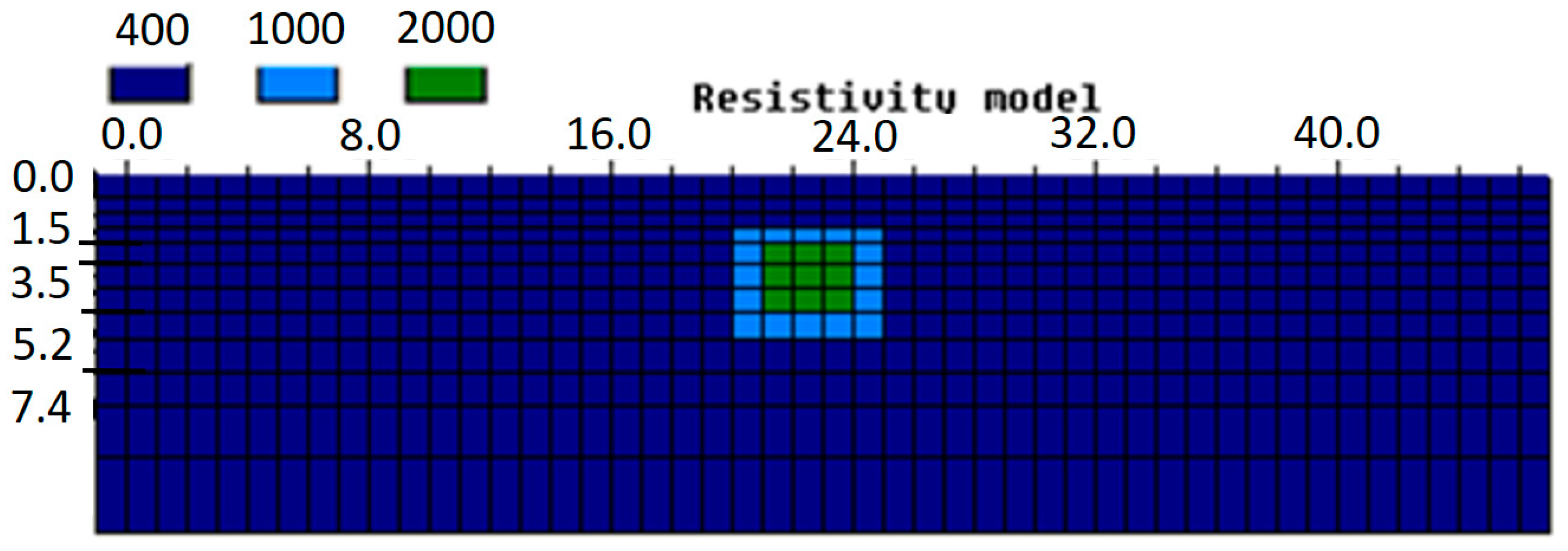
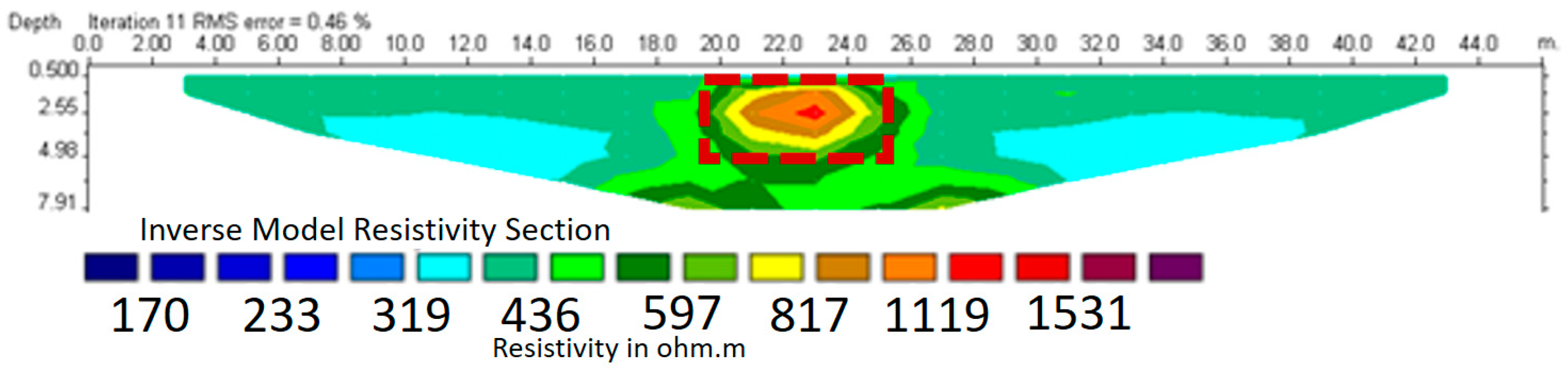
2.2. Reliability Analysis

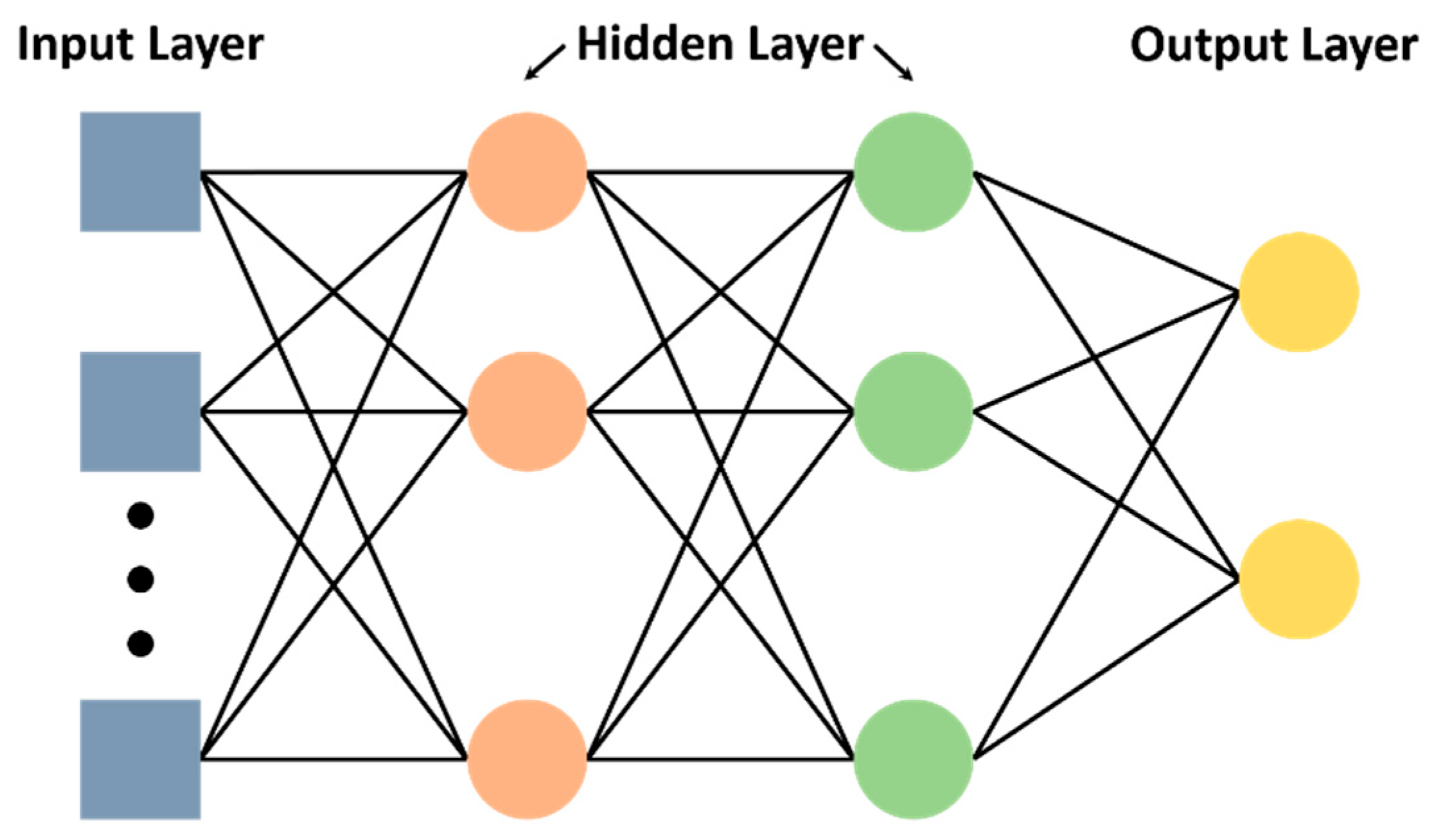
To analyse the reliability of the 2D-ERT result, this study attempts to build a numerical model to validate the correctness of in situ measured data. The numerical model was built using RES2DMOD developed by Geotomo [46]. The in situ geologic configuration was simulated in the built mesh, and an appropriate resistivity value was given. The numerical solution was calculated using the finite element method to obtain apparent resistivity, and the apparent resistivity profile inverse calculation was carried out using the Optimal least square method (Res2dinv [47]). The numerical simulation resistivity profile can be obtained and compared with the in situ actual resistivity profile result.

The numerical model resistivity can be obtained from the collected geologic data, such as geologic maps, drilling data, the resistivity distribution range of geomaterial, and the preliminary detection result of ERT. Different depths, positions, or specific regions of the model are given appropriate resistivity values according to experience and professional judgment.

According to the analysis of the collected geologic data of the site, the geology around the Shuangru Mountain Tunnel mainly comprises two kinds of strata, which are silty sand within 15 m below the earth’s surface and silty clay at 15–30 m below the earth’s surface. This study referred to the geologic drilling data of the site and took the silty sand as background to build the numerical model of a tunnel and simulate the tectonics stratum of the tunnel.

2.3. Deep Learning

The MLP is one of the basic types of deep learning architecture. Its architecture follows the neural network system principle, learns, and predicts data. The MLP learns in the perceptron; the weight is changed after each data processing. The weight is adjusted using an algorithm, and the deviation in the training process is reduced to minimize the error in the amount of output and prediction results. The main advantage is the ability to solve complex problems rapidly. The MLP is a feedforward neural network composed of the multilayer structure of linear and nonlinear activation functions. Each layer is composed of basic elements of neurons, and each neuron is fully connected to all others in the previous and subsequent layers. Neurons in the network have a bias value b and an activation function f. The connection between neurons in different layers is defined by connection weight, $w_i\in R, i\in \left\{1,2,\dots ,n\right\}$. These parameters are updated during the training of MLP. The general activation functions are ReLU, TANH, sigmoid, and softmax. The output value y of a neuron is defined as:

$$y=f\left({\displaystyle \sum }_{i=1}^n{w}_i{x}_i+b\right)$$

(1)

where $x_i$ is the output value of neuron i of the previous layer, $i\in \left\{1,2,\dots ,n\right\}$. The MLP network generally includes one input layer, one output layer, and one or more dense layers, detailed below.

• Input layer: the number of neurons of the input layer is determined by the point k of input data.
• Hidden layer: fully connected layer between the input layer and output layer.
• Output layer: the neuron of the output layer is determined by the number of classes or the output of the approximation function.

In the training process of MLP, the weight $w_i$ and offset parameter b are updated in every iteration, and the update target is a minimum loss function. After network training, it can be used for classification or function approximation. The architecture is shown in Figure 2 [48,49,50,51,52].

In this study, we used Adaptive Moment Estimation (Adam) optimization to train MLP and minimize the Mean Squared Error (MSE). Adam optimization was applied to calculate the adaptive training rate of the parameters [53]. This method, in addition to storing the descending mean of the square of the past of the gradient or $v_t$ and the mean of the descending of the past of the gradient or $m_t$, is kept as momentum. This is why the momentum can be seen as a ball sliding on a sloping surface with no friction and, therefore, can be placed at the minimum error level [54]. Both parameters of the mean descending average of the square of the gradient and the average of the descending of the past of the gradient can be calculated as follows:

$$m_t={\beta }_1{m}_{t-1}+\left(1-{\beta }_1\right)g_t$$

$$v_t={\beta }_2{v}_{t-1}+\left(1-{\beta }_2\right)g_t^2$$

where $g_t$ is the gradients at subsequent time steps, $m_t$ and $v_t$ are estimates of the first moment (the mean) and the second moment (the uncentered variance) of the gradients, respectively (hence the name of the method). As $m_t$ and $v_t$ are initialized as vectors of zeros, the authors of Adam observe that they are biased towards zero, especially during the initial time steps, especially when the decay rates are low (i.e., ${\beta }_1$ and ${\beta }_2$ are close to 1).

The prediction of unknown data has always been a complex problem, and it is also an important application in neural networks. The high-level network architecture of deep learning can more accurately predict and describe the distribution and changes of unknown data. The ERT profile is an inverted trapezoid; two sides are blank and short of resistivity data. This study used machine learning, data prediction, and computational ability to reduce the error between the actual value and prediction value of MLP for the blank in the field test ERT profile by MLP. The result was obtained after reiteration to convergence, forming a complete rectangular section. More profiles of different positions were developed from MLP, and the in situ 3D resistivity model was built last. In this study, we used only three-layer (discrete) 2D-ERT data to predict that multilayer (continuous) 3D ERT data is itself a complex and challenging problem. We hope that the 3D resistivity image predicted by MLP will enhance image resolution and interpretation capability.

3. Results and Discussion

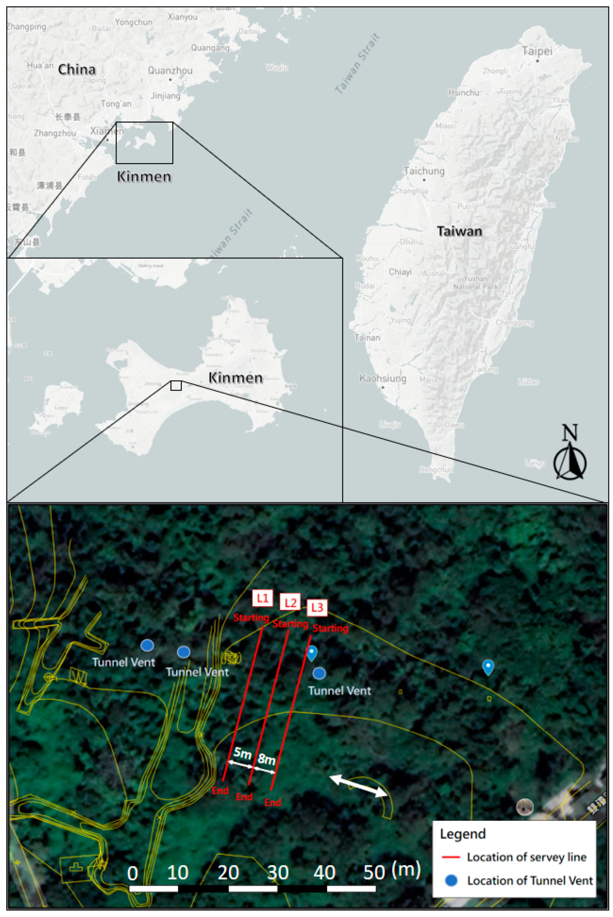
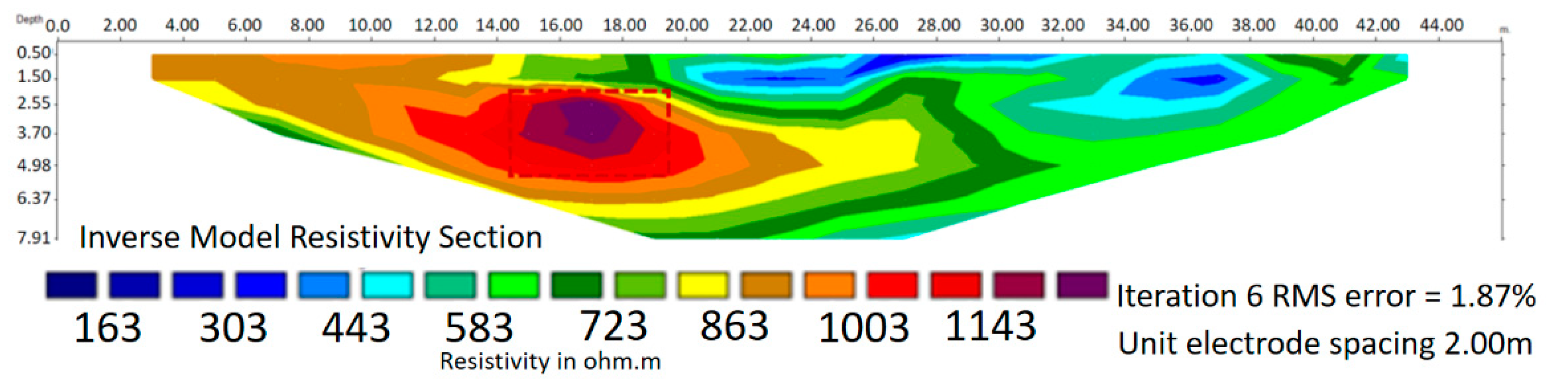
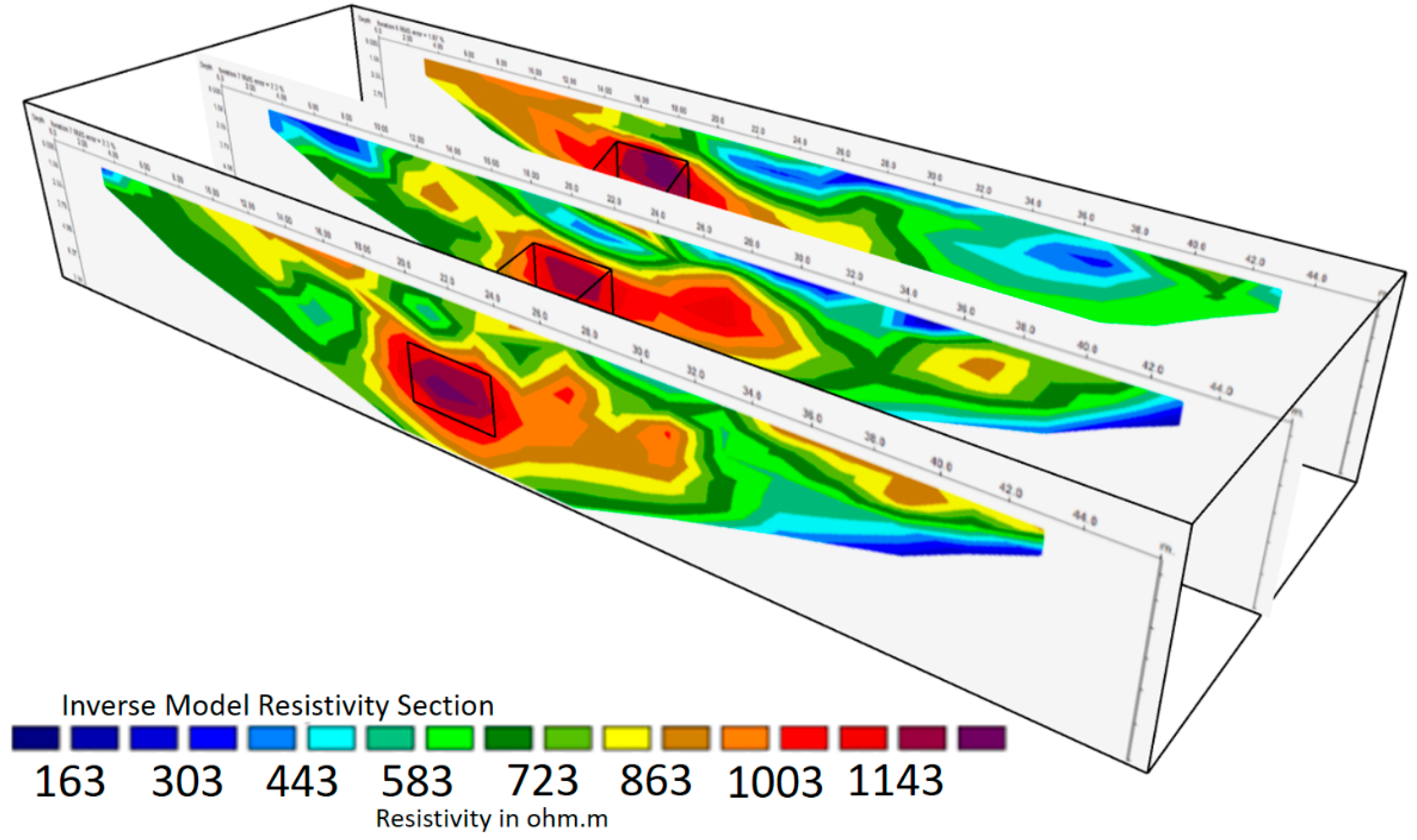
3.1. ERT Field Acquisition and Data Analysis

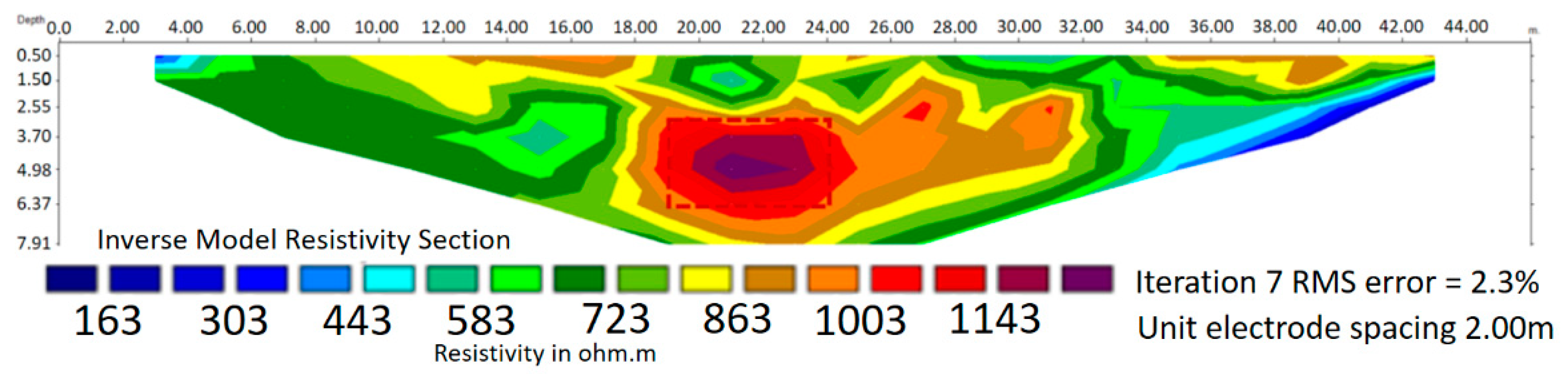
3.1.1. L1 Survey Line

The result of the L1 survey line, according to Wenner, is shown in Figure 3 (RMS Error = 2.3%). The electrical property of the stratum is approximately divided into two layers, and the resistivity profile descends as the depth increases. There are two higher resistivity regions located at the survey line 10–18 m and 34–42 m, within 1.5 m depth from the surface. Because Kinmen Island had been free of rain for a long time in the measurement period, the topsoil was very dry. The other region shows low resistivity values at 3–18 m and 32–42 m of survey line and within 1.5–7.9 m underground. As the geology of this region is silty sand stratum, the geology is relatively loose and has higher water content. Notably, at 18–25 m of survey line and 2.5–6.5 m of depth, the resistivity value increases suddenly, the resistivity value of this region increases inwards, indicating this may be the tunnel location, according to preliminary analysis. According to Figure 3, the tunnel may be located at 2.5 m underground, with a height of about 2.5 m and a width of about 4 m, indicated by red dotted lines in Figure 3.

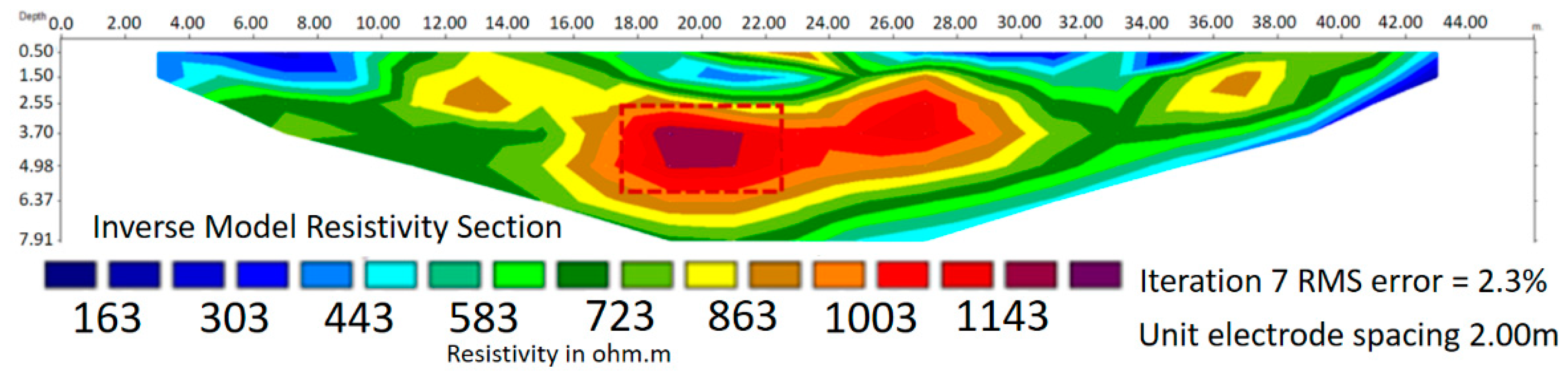
3.1.2. L2 Survey Line

Figure 4 shows the result of the L2 survey line (RMS Error = 2.3%). It shows the same trend as Figure 3 because the L2 survey line is close to L1. The stratum is divided into two layers, in which the middle region has relatively high resistivity, while the rest is a stratum of lower resistivity. As the geology of this region is silty sand stratum, the geology is relatively loose and has higher water content. At 18–28 m of survey line and 2.5–5.5 m of depth, the resistivity value increases suddenly, the resistivity value of this region increases inwards, indicating this may be the tunnel location according to preliminary analysis. As shown in Figure, the tunnel may be located at 2.5 m underground, with a height of about 2.5 m and width of about 4 m, indicated by red dotted lines in Figure 4.

3.1.3. L3 Survey Line

The result of the L3 survey line, according to Wenner, is shown in Figure 5 (RMS Error = 1.87%). It shows the same trend as Figure 4 because of the proximity of the L3 survey line to L2. The electrical property of the stratum is approximately divided into two layers. The resistivity profile descends as the depth increases, and there is a region of relatively high resistivity in the middle. At 3–14 m of survey line and within the earth’s surface to 1.5 m underground, this region showed higher resistivity. Because Kinmen Island had been free of rain for an extended period during measurement, the topsoil was extremely dry. The other region showed a low resistivity value at 22–42 m of survey line and within the distance of 7.9 m from the earth’s surface. As the geology of this region is silty sand stratum, the geology is relatively loose and has higher water content. At 12–20 m of the survey line and 2–5 m of depth, the resistivity value increases suddenly, and the resistivity value of this region increases inwards. This indicates a possible tunnel location, according to preliminary analysis. As shown in Figure 5, the tunnel may be located at 2 m underground, the height is about 2.5 m, and the width is about 4 m, indicated by red dotted lines in Figure 5.

3.1.4. Comprehensive Interpretation

According to the measurement results of three survey lines, L1, L2, and L3, there is a high resistivity region in the earth resistivity profile. In order to analyse whether the high resistivities are correlated with each other in space, a 2.5D simulated diagram of the three survey lines in relative positions is drawn, as shown in Figure 6. It is observed that if the high resistivity regions of various profiles are selected and connected in line, the selected region and path correspond to the tunnel location and path in the literature.

3.2. Reliability Analysis

To verify the reliability of the 2D-ERT images, this study constructed a numerical model to validate the correctness of in situ measured data. To simulate the onsite strata condition, this study used the same measurement parameters as in situ measurement, referred to the geologic drilling data of site, and took the silty sand as background to build the numerical model of a tunnel to simulate the stratum tectonics of the tunnel in the stratum. Referring to the site concrete tunnel size, a 3 m high and 5 m wide square tunnel was built at 2 m underground, and the reasonable resistivity of each unit was assumed. The resistivity value of the concrete tunnel was assumed to be 1000 ohm-m, dry air inside a tunnel, the resistivity was assumed to be 2000 ohm-m, the resistivity of the soil layer covering the tunnel was assumed to be 400 ohm-m. The numerical model is shown in Figure 7.

Figure 8 shows the numerical simulation result (RMS Error = 0.46%). As seen, the background silty sand shows low resistivity distribution, and relatively low resistivity values are shown at 2–18 m and 26–42 m of the survey line. Relatively high resistivity distribution is shown at 20–25 m of a survey line and 2–5 m of depth, indicated by red dotted lines in Figure 8. The numerical simulation result in Figure 8 is compared with the in situ test results in Figure 3, Figure 4 and Figure 5. The four figures are very similar to each other, proving that the stratum tectonics in Figure 3, Figure 4 and Figure 5 match the stratum tectonics assumed by numerical simulation, proving high reliability. Therefore, the high resistivity region is identified as the tunnel location and path.

4. Deep Learning Prediction

The 2D ERT test result mainly shows a 2D profile; the tunnel location and path cannot be interpreted directly. To establish a 3D electrical resistivity model, this study used MLP for calculation. The computational ability of learning, data prediction, and reducing the error between the actual value and prediction value of MLP was used to build the in situ 3D electrical resistivity model.

Figure 9a–g shows a series of results of deep learning prediction. Before artificial intelligence calculation, the measured data in this research must be converted into an MLP data format. The L1, L2, and L3 in situ measurement results are inputted to establish the graph of the relation of relative positions of L1, L2, and L3 for the initial model. Figure 9a shows the initial model of the original data of L1, L2, and L3; the result is similar to Figure 6.

Table 1. MLP network structure parameter list.

Structure	Parameter
Number of layers	3
Number of Neurons in the layers	Input = 2, Hidden1 = 32, Hidden2 = 32 Output = 1
Initial weights and biases	Random
Activation function	Sigmoid
Optimization	Adam

shows the MLP network structure parameters. The MLP is a three-layer architecture, including two hidden and one output layer. Figure 9b shows the training result of the MLP network. The MLP is reiterated during training to reduce the error amount of output and prediction results and performs calculations until the network converges. Through the nonlinear iterative calculation of the MLP, as seen in Figure 9b, the error value is converged slowly after each iterative computation. Figure 9c shows the result of the original data after MLP data prediction. This is the output of the training data, which can be compared with the original data in Figure 9a. It can be seen that the training results can faithfully present the original data characteristics. Figure 9d shows the results of using the trained MLP to predict the unknown regions of L1, L2, and L3. Figure 9d shows the initially blank areas and without onsite measurement data, such as the lower left corner and the lower right corner, which can be predicted by the MLP network to predict the resistance value. Figure 9e shows the result of using the trained MLP to predict successive profiles. When the predicted number of profiles increases, the 3D resistivity model is built, and 14 profiles are predicted in this study. Due to the narrow scope of this study, the 14 layers of data are predicted by three layers of original data of the resistivity values predicted by the MLP network, which is sufficient to establish a 3D model. Figure 9f shows the 3D resistivity model result. The tunnel is a reinforced concrete structure; it is characterized by unlikely electrical conduction and high resistivity, especially in the 2D ERT result. In order to highlight the location of high resistivity, this study concealed the low resistivity colour of the 3D resistivity model in Figure 9f. After repeated tests and the resistivities are arranged, the 60% of the resistance value is taken as a boundary, the colour of resistivity value lower than 60% is hidden, and the colour of resistivity value higher than 60% is displayed. The result, after adjustment, is shown in Figure 9g; the tunnel location and path have been shown clearly.

From the existing literature, we already know the approximate location and direction of the underground tunnel in reality. The results of the MLP study show that a few (three layers) 2D-ERT data to predict the 3D ERT data can be seen and that the location of the tunnel is consistent with the actual location.

5. Conclusions

Most of the extensively hidden underground tunnels in Kinmen Island have been abandoned and unoccupied to avoid the damage to human life and property caused by tunnel breakdown and prevent accidental destruction of the precious cultural heritage. This study used 2D-ERT for in situ measurement to find the location of tunnels hidden underground. To test the reliability of 2D-ERT in tunnel survey, a numerical model was built. The actual configuration of the onsite strata and the shape of the underground tunnel were simulated to analyze and validate the accuracy of in situ measurement. In addition, to enhance the measurement result interpretation ability and resolution to determine the actual position and path of the tunnel, this study used an artificial intelligence algorithm to estimate and build a 3D electrical resistivity model.

The results indicate that three survey lines were used for 2D ERT measurement in this study. As the tunnel is a reinforced concrete structure, it is characterized by unlikely electrical conduction and high resistivity, especially in the 2D ERT result. The three survey lines have high resistivity regions in the profiles. According to the numerical simulation result, this high resistivity region is highly likely to be the tunnel location, and the tunnel location, height, and width have been displayed clearly. The three survey lines are displayed in 2.5D mode. The high resistivity regions of various profiles are selected and connected in line, and the selected region and path are similar to in situ tunnel location and path. According to the results of this study, using 2D-ERT to survey underground tunnels is highly feasible.

With the 2D-ERT test result showing a 2D profile, the tunnel location and path cannot be interpreted directly. As the 3D electrical resistivity survey is limited by space, time, and economy, the measurement is not yet frequently used. In recent years, artificial intelligence has been extensively used in various domains. To establish a 3D resistivity map, this study used the MLP of artificial intelligence deep learning algorithm for calculation and used the computational ability of learning, data prediction. The error between the actual value and prediction value of MLP was reduced to complete the building of in situ 3D electrical resistivity model. According to a series of findings, the tunnel location and path can be displayed using an artificial intelligence algorithm. The measurement result interpretation ability and resolution are enhanced effectively. This study can further discuss different types of tunnels in the future to enhance the feasibility of 2D-ERT for underground tunnel surveys.

References

1. Chiang, B.W. Investigation and Research of Kinmen Wars Records; Kinmen National Park: Kinmen, Taiwan, 2005. [Google Scholar]
2. The Underground Tunnels Collapsed and Endangered the Houses, Kinmen Daily. 2014. Available online: https://www.chinatimes.com/realtimenews/20140523003816-260402?chdtv (accessed on 30 October 2021).
3. The Government Public Works Were Stopped Construction by Underground Tunnels during Excavation, Liberty Times. 2018. Available online: https://www.kmdn.gov.tw/1117/1271/1272/136247/ (accessed on 30 October 2021).
4. The Government Public Works Were Found Ammunition Galleries during Excavation, Kinmen Daily. 2006. Available online: https://www.kmdn.gov.tw/1117/1271/1272/136098/?cprint=pt (accessed on 30 October 2021).
5. Raffaele Persico Salvatore Piro Neil Linford, Innovation in Near Surface Geophysics; Elsevier: Amsterdam, The Netherlands, 2018; ISBN 9780128124307.
6. Lin, C.P.; Lin, C.H.; Wu, P.L.; Liu, H.C.; Hung, Y.C. Applications and challenges of near surface geophysicals in geotechnical engineering. Chin. J. Geophys. 2015, 58, 2664–2680. [Google Scholar]
7. Lin, C.H.; Lin, C.P.; Hung, Y.C.; Chung, C.C.; Wu, P.L.; Liu, H.C. Application of geophysical methods in a dam project: Life cycle perspective and Taiwan experience. J. Appl. Geophys. 2018, 158, 82–92. [Google Scholar] [CrossRef]
8. Stokoe, K.H.; Joh, S.H.; Woods, R.D. Some contribution of in situ geophysical measurements to solving geotechnical engineering problems. In Proceedings of the 2nd International Geotechnical and Geophysical Site Characterization Conference, ISC-2, Porto, Portugal, 19–22 September 2004; pp. 97–132. [Google Scholar]
9. Geophysical Survey System, Inc. Traning Notes; GSSI Press: Nashua, NH, USA, 1992. [Google Scholar]
10. Geophysical Survey System, Inc. RADAN for Windows Version 5.0 User’s Manual; GSSI Press: Nashua, NH, USA, 2003; pp. 1–132. [Google Scholar]
11. Ribolini, A.; Bini, M.; Isola, I.; Coschino, F.; Baroni, C.; Salvatore, M.C.; Zanchetta, G.; Fornaciati, A. GPR versus geoarchaeological findings in a complex archaeological site (Badia Pozzeveri, Italy). Archaeol. Prospect. 2017, 24, 141–156. [Google Scholar] [CrossRef]
12. Lee, D.H.; Lai, S.L.; Wu, J.H.; Chang, S.K.; Dong, Y.M. Detecting the remaining structure foundation using ground penetrating radar: The outer wall of small east gate of Taiwan FU, Taiwan. J. GeoEng. 2018, 13, 85–92. [Google Scholar] [CrossRef]
13. Baryshnikov, V.D.; Khmelin, A.P.; Denisova, E.V. GPR detection of inhomogeneities in concrete lining of underground tunnels. J. Min. Sci. 2014, 50, 25–32. [Google Scholar] [CrossRef]
14. Li, S.C.; Zhou, Z.Q.; Ye, Z.H.; Li, L.P.; Zhang, Q.Q.; Xu, Z.H. Comprehensive geophysical prediction and treatment measures of karst caves in deep buried tunnel. J. Appl. Geophys. 2015, 116, 247–257. [Google Scholar] [CrossRef]
15. Mochales, T.; Casas, A.M.; Pueyo, E.L.; Pueyo, O.; Román, M.T.; Pocoví, A.; Soriano, M.A.; Ansón, D. Detection of underground cavities by combining gravity, magnetic and ground penetrating radar surveys: A case study from the Zaragoza area, NE Spain. Environ. Geol. 2008, 53, 1067–1077. [Google Scholar] [CrossRef]
16. Karlovsek, J.; Scheuermann, A.; Willimas, D.J. Investigation of voids and cavities in bored tunnels using GPR. In Proceedings of the 2012 14th International Conference on Ground Penetrating Radar (GPR), Shanghai, China, 4–8 June 2012; pp. 496–501. [Google Scholar]
17. Gracia, V.P.; Canas, J.A.; Pujades, L.G.; Clapés, J.; Caselles, O.; Garcıa, F.; Osorio, R. GPR survey to confirm the location of ancient structures under the Valencian Cathedral (Spain). J. Appl. Geophys. 2000, 43, 167–174. [Google Scholar] [CrossRef]
18. Leucci, G.; Parise, M.; Sammarco, M.; Scardozzi, G. The Use of Geophysical Prospections to Map Ancient Hydraulic Works: The Triglio Underground Aqueduct (Apulia, Southern Italy): GPR and ERT Survey on Ancient Hydraulic Works. Archaeol. Prospect. 2016, 23, 195–211. [Google Scholar] [CrossRef]
19. Dahlin, T. The development of DC resistivity imaging techniques. Comput. Geosci. 2001, 27, 1019–1029. [Google Scholar] [CrossRef] [Green Version]
20. Hung, Y.C.; Chou, H.S.; Lin, C.P. Appraisal of the Spatial Resolution of 2D Electrical Resistivity Tomography for Geotechnical Investigation. Appl. Sci. 2020, 10, 4394. [Google Scholar] [CrossRef]
21. Suzuki, K.; Toda, S.; Kusunoki, K.; Fujimitsu, Y.; Mogi, T.; Jomori, A. Case studies of electrical and electromagnetic methods applied to mapping active faults beneath the thick quaternary. Eng. Geol. 2000, 56, 29–45. [Google Scholar] [CrossRef]
22. Demanet, D.; Renardy, F.; Vanneste, K.; Jongmans, D.; Camelbeeck, T.; Meghraoui, M. The use of geophysical prospecting for imaging active faults in the Roer Graben, Belgium. Geophysics 2001, 66, 78–89. [Google Scholar] [CrossRef]
23. Batayneh, A.; Barjous, M. A Case Study of Dipole-Dipole Resistivity for Geotechnical Engineering from the Ras en Naqab Area, South Jordan. J. Environ. Eng. Geophys. 2003, 8, 31–38. [Google Scholar] [CrossRef]
24. Rizzoa, E.; Colellab, A.; Lapennaa, V.; Piscitellia, S. High resolution images of the fault controlled High Agri Valley basin (Southern Italy) with deep and shallow electrical resistivity tomographies. Phys. Chem. Earth 2004, 29, 321–327. [Google Scholar] [CrossRef]
25. Nguyen, F.; Garambois, S.; Jongmans, D.; Pirard, E.; Loke, M.H. Image processing of 2D resistivity data for imaging faults. J. Appl. Geophys. 2005, 57, 260–277. [Google Scholar] [CrossRef]
26. Pazzi, V.; Morelli, S.; Fanti, R. A Review of the Advantages and Limitations of Geophysical Investigations in Landslide Studies. Int. J. Geophys. 2019, 2019, 2983087. [Google Scholar] [CrossRef] [Green Version]
27. Batayneh, A.; Al-Diabat, A.A. Application of a two dimensional electrical tomography technique for investigating landslides along the Amman–Dead Sea highway, Jordan. Environ. Geol. 2002, 42, 399–403. [Google Scholar] [CrossRef]
28. Perrone, A.; Iannuzzi, A.; Lapenna, V.; Lorenzo, P.; Piscitelli, S.; Rizzo, E.; Sdao, F. High resolution electrical imaging of the Varco d’Izzo earthflow (southern Italy). J. Appl. Geophys. 2004, 56, 17–29. [Google Scholar] [CrossRef]
29. Chen, T.T.; Hung, Y.C.; Hsueh, M.W.; Yeh, Y.H.; Weng, K.W. Evaluating the Application of Electrical Resistivity Tomography for Investigating Seawater Intrusion. Electronics 2018, 7, 107. [Google Scholar] [CrossRef] [Green Version]
30. Nyquist, J.E.; Bradley, J.C.; Davis, R.K. DC resistivity monitoring of potassium permanganate injected to oxidize TCE in situ. J. Environ. Eng. Geophys. 1999, 4, 135–148. [Google Scholar] [CrossRef]
31. Lin, C.-P.; Hung, Y.-C.; Yu, Z.-H. Performance of 2D ERT in Investigation of Abnormal Seepage: A Case Study at the Hsin-Shan Earth Dam in Taiwan. J. Environ. Eng. Geophys. 2014, 9, 101–112. [Google Scholar] [CrossRef]
32. Hung, Y.C.; Chen, T.T.; Tsai, T.F.; Chen, H.X. A Comprehensive Investigation on Abnormal Impoundment of Reservoirs—A Case Study of Qionglin Reservoir in Kinmen Island. Water 2021, 13, 1463. [Google Scholar] [CrossRef]
33. Colucci, P.; Darilek, G.T.; Laine, D.L.; Binley, A. Locating Landfill Leaks Covered with Waste. In Proceedings of the International Waste Management and Landfill Symposium, Sardinia 99, Cagliari, Italy, 4–8 October 1999; Volume 3, pp. 137–140. [Google Scholar]
34. Binley, A.; Daily, W.; Ramirez, A. Detecting leaks from waste storage ponds using electrical tomographic methods. In Proceedings of the 1st World Congress on Process Tomography, Buxton, UK, 14 April 1999; pp. 6–17. [Google Scholar]
35. Daily, W.; Ramirez, A.; Binley, A. Remote Monitoring of Leaks in Storage Tanks using Electrical Resistance Tomography: Application at the Hanford Site. J. Environ. Eng. Geophys. 2004, 9, 11–24. [Google Scholar] [CrossRef]
36. Orfanos, C.; Apostolopoulos, G. 2D-3D resistivity and microgravity measurements for the detection of an ancient tunnel in the Lavrion area, Greece. Near Surf. Geophys. 2011, 9, 449–457. [Google Scholar] [CrossRef]
37. Mousavi, H.; Khazaei, S. Detection of underground tunnels using electrical resistivity and refraction seismic tomography methods. J. Earth Space Phys. 2016, 42, 578–606. [Google Scholar]
38. Lesparre, N.; Boyle, A.; Grychtol, B.; Cabrera, J.; Marteau, J.; Adler, A. Electrical resistivity imaging in transmission between surface and underground tunnel for fault characterization. J. Appl. Geophys. 2016, 128, 163–178. [Google Scholar] [CrossRef]
39. Loke, M.H. Tutorial: 2-D and 3-D Electrical Imaging Surveys; Geotomo Software: Penang, Malaysia, 2004. [Google Scholar]
40. Pouyanfar, S.; Sadiq, S.; Yan, Y.; Tian, H.; Tao, Y.; Reyes, M.P.; Shyu, M.L.; Chen, S.C.; Iyengar, S.S. A survey on deep learning: Algorithms, techniques, and applications. ACM Comput. Surv. (CSUR) 2018, 51, 1–36. [Google Scholar] [CrossRef]
41. Alile, O.M.; Aigbogun, C.O.; Enoma, N.; Abraham, E.M.; Ighodalo, J.E. 2D and 3D Electrical Resistivity Tomography (ERT) Investigation of Mineral Deposits in Amahor, Edo State, Nigeria. Niger. Res. J. Eng. Environ. Sci. 2017, 2, 215–231. [Google Scholar]
42. Alile, O.M.; Abraham, E.M. Three dimensional geoelectrical imaging of the subsurface structure of university of Benin-Edo state Nigeria. Adv. Appl. Sci. Res. 2015, 6, 85–93. [Google Scholar]
43. Bentley, L.R.; Gharibi, M. Resistivity Imaging at a Heterogeneous Two and Three Dimensional Electrical Remediation Site. Geophysics 2004, 69, 674–680. [Google Scholar] [CrossRef]
44. Chávez, R.E.; Cifuentes Nava, G.; Tejero, A.; Hernández Quintero, J.E.; Vargas, D. Special 3D electric resistivity tomography (ERT) array applied to detect buried fractures on urban areas: San Antonio Tecómitl, Milpa Alta, México. Geofísica Int. 2014, 53, 425–434. [Google Scholar] [CrossRef] [Green Version]
45. Osinowo, O.O.; Falufosi, M.O. 3D Electrical Resistivity Imaging (ERI) for subsurface evaluation in pre engineering construction site investigation. NRIAG J. Astron. Geophys. 2018, 7, 309–317. [Google Scholar] [CrossRef]
46. Geotomo Software 2002. RES2DMOD Ver. 3.01, Rapid 2D Resistivity forward Modelling Using the Finite Difference and Finite-Element Methods. Available online: https://www.geotomosoft.com/index.php (accessed on 30 October 2021).
47. Geotomo Software 2007. RES2DINV Ver. 3.56, Rapid 2D Resistivity and IP Inversion Using the Least Squares Method. Available online: https://www.geotomosoft.com/index.php (accessed on 30 October 2021).
48. Russell, S.; Norvig, P. Artificial Intelligence: A Modern Approach. 2002. Available online: https://storage.googleapis.com/pub-tools-public-publication-data/pdf/27702.pdf (accessed on 30 October 2021).
49. Rojas, R. Neural Networks: A Systematic Introduction; Springer Science & Business Media: Berlin/Heidelberg, Germany, 2013. [Google Scholar]
50. Nilsson, N.J. Principles of Artificial Intelligence; Morgan Kaufmann: Burlington, MA, USA, 2014. [Google Scholar]
51. LeCun, Y.; Bengio, Y.; Hinton, G. Deep learning. Nature 2015, 521, 436–444. [Google Scholar] [CrossRef] [PubMed]
52. Goodfellow, I.; Bengio, Y.; Courville, A. Deep Learning; MIT Press: Cambridge, MA, USA, 2016. [Google Scholar]
53. Kingma, D.P.; Ba, J.L. Adam: A Method for Stochastic Optimization. In Proceedings of the International Conference on Learning Representations, San Diego, CA, USA, 7–9 May 2015; pp. 1–13. [Google Scholar]
54. Heusel, M.; Ramsauer, H.; Unterthiner, T.; Nessler, B.; Hochreiter, S. GANs Trained by a Two Time Scale Update Rule Converge to a Local Nash Equilibrium. Adv. Neural Inf. Processing Syst. 2017, 30, 1–12. [Google Scholar]
Figure 1. Test site location and measurement wiring diagram.
Applsci 12 00639 g001
Figure 2. MLP architecture diagram.
Applsci 12 00639 g002
Figure 3. L1 result.
Applsci 12 00639 g003
Figure 4. L2 result.
Applsci 12 00639 g004
Figure 5. L3 result.
Applsci 12 00639 g005
Figure 6. 2.5D simulated diagram of three survey lines.
Applsci 12 00639 g006
Figure 7. Numerical simulation model.
Applsci 12 00639 g007
Figure 8. Numerical simulation result.
Applsci 12 00639 g008
Figure 9. Deep learning prediction results (ag). (a) Original data of L1, L2, and L3; (b) Error rate of MLP network training process; (c) Result of the original data of L1, L2, and L3 after MLP data prediction; (d) Result of unknown regions of L1, L2, and L3 after MLP data prediction; (e) Result of successive profiles after MLP data prediction; (f) Result of 3D resistivity model; (g) MLP predicted tunnel location and path.
Applsci 12 00639 g009aApplsci 12 00639 g009bApplsci 12 00639 g009cApplsci 12 00639 g009dApplsci 12 00639 g009e