In this section, we describe the hybrid ASR systems developed by the MLLP-VRAIN that participated in the Albayzín-RTVE 2020 S2T Challenge.
3.2. Language Modelling
Regarding language modelling, we trained count-based (n-gram) and neural-based (LSTM, Transformer) language models (LMs) to perform one-pass decoding with different linear combinations of them [
16], using the text data sources and corpora described in
Table 2.
On the one hand, we trained 4-gram LMs using SRILM [
36] with all text resources plus the Google-counts v2 corpus [
37], accounting for 102G running words. The vocabulary size was limited to 254 K words, with an OOV ratio of
% computed over our internal development set.
On the other hand, regarding neural LMs, we considered the LSTM and Transformer architectures. In both cases, LMs were trained using a 1-gigaword subset randomly extracted from all available text resources, except Google-counts. Their vocabulary was defined as the intersection between the n-gram vocabulary (254 K words) and that derived from the aforementioned training subset. We did this to avoid having zero probabilities for words that are present in the system vocabulary but not in the training subset. This is taken into account when computing perplexities by renormalizing the unknown-word score accordingly.
Specific training details for each neural LM architecture are as follows. Firstly, LSTM LMs were trained using the CUED-RNNLM toolkit [
38]. The Noise Contrastive Estimation (NCE) criterion [
39] was used to speed up model training, and the normalization constant learned from training was used during decoding [
40]. Based on the lowest perplexity observed on our internal development set, a model with a 256-unit embedding layer and two hidden LSTM layers of 2048 units was selected. Secondly, Transformer LMs (TLMs) were trained using a customized version of the FairSeq toolkit [
41], with the following configuration minimizing perplexity in our internal development set: 24-layer network with 768 units per layer, 4096-unit feed-forward neural network, 12 attention heads, and an embedding of 768 dimensions. These models were trained until convergence with batches limited to 512 tokens. Parameters were updated every 32 batches. During inference, Variance Regularization was applied to speed up the computation of TLM scores [
21].
Table 2.
Statistics of Spanish text resources for LM training. S = Sentences, RW = Running words, V = Vocabulary. Units are in thousands (K).
Table 2.
Statistics of Spanish text resources for LM training. S = Sentences, RW = Running words, V = Vocabulary. Units are in thousands (K).
| Corpus | S (K) | RW (K) | V (K) |
|---|
| OpenSubtitles [42] | 212,635 | 1,146,861 | 1576 |
| UFAL [43] | 92,873 | 910,728 | 2179 |
| Wikipedia [44] | 32,686 | 586,068 | 3373 |
| UN [45] | 11,196 | 343,594 | 381 |
| News Crawl [46] | 7532 | 198,545 | 648 |
| Internal: entertainment | 4799 | 59,235 | 307 |
| eldiario.es [47] | 1665 | 47,542 | 247 |
| El Periódico [48] | 2677 | 46,637 | 291 |
| Common Crawl [49] | 1719 | 41,792 | 486 |
| Internal: parliamentary data | 1361 | 35,170 | 126 |
| News Commentary [46] | 207 | 5448 | 83 |
| Internal: educational | 87 | 1526 | 35 |
| TOTAL | 369,434 | 3,423,146 | 5785 |
| Google-counts v2 [37] | - | 97,447,282 | 3693 |
3.3. Decoding Strategy
Our hybrid ASR systems follow a real-time one-pass decoding by means of a History Conditioned Search (HCS) strategy, as described in [
16]. HCS groups hypotheses by their LM history, with each group representing all state hypotheses sharing a common history. In this way, word histories only need to be considered when handling word labels, and thus can be ignored during dynamic programming at intra-word state level [
50]. This approach allows us to benefit from the direct usage of additional LMs during decoding while satisfying real-time constraints. This decoding strategy introduces two additional and relevant parameters to control the trade-off between Real-Time Factor (RTF) and WER: LM history recombination, and LM histogram pruning. The static look-ahead table, needed by the decoder to use pre-computed look-ahead LM scores, is generated from a pruned version of the n-gram LM.
For streaming ASR, as the full sequence (context) is not available during decoding, BLSTM AMs are queried with a sliding, overlapping context window of limited size over the input sequence, averaging outputs of all windows for each frame to obtain the corresponding acoustic score [
20]. The size of the context window (in frames or seconds) is set in decoding, and defines the theoretical latency of the system. This limitation of the context prevents us from performing a Full Sequence Normalization, which is typically applied under the off-line setting. Instead, we applied the Weighted Moving Average (WMA) technique, which uses the content of the current context window to update normalization statistics on-the-fly [
51]. This technique is applied over a batch
of frames as
where
being
the accumulated values of previous frames until batch
,
the
t-th frame in batch
,
the number of frames until batch
, and
b and
w the batch and window sizes, respectively.
and
are accumulated values that are updated by weighting the contribution of previous batches with an adjustable parameter
:
Finally, as Transformer LMs have the inherent capacity of attending to potentially infinite word sequences, history is limited to a given maximum number of words, in order to meet the strict computational time constraints imposed by the streaming scenario [
21]. By applying all these modifications, our decoder acquires the capacity to deliver live transcriptions for incoming audio streams of potentially infinite length, with latencies lower-bounded by the context window size.
3.4. Experiments and Results
To carry out and evaluate our system development, we used the dev and test sets from the RTVE2018 database. For the experiments, we devoted our internally split
dev1-dev set [
28] for development purposes, whilst
dev2 and
test-2018 were used to test ASR performance. Finally,
test-2020 was the blind test used by the organisation to rank the participant systems.
Table 3 provides basic statistics of these sets.
First, we studied the perplexity (PPL) on the
dev1-dev set of all possible linear combinations for the three types of LMs considered in this work.
Table 4 shows the PPLs of these interpolations, along with the optimum LM weights that minimized PPL in the
dev1-dev set. The Transformer LM provides significantly lower perplexities in all cases and, accordingly, takes very high weight values when combined with other LMs. Indeed, the TLM in isolation already delivers a strong perplexity baseline value of 63.3, while the maximum PPL improvement is just 6% relative when all three LMs are combined.
Second, we tuned decoding parameters to provide a good WER-RTF tradeoff on dev1-dev, with the hard constraint of RTF < 1 to ensure real-time processing of the input. From these hyperparameters, we highlight, due to their relevance, a LM history recombination of 12, LM histogram pruning of 20, and TLM history limited to 40 words.
At this point, we defined our participant off-line hybrid ASR system identified as
c3-offline (contrastive system no. 3), consisting of a fast pre-recognition + Voice Activity Detection (VAD) step to detect speech/non-speech segments as in [
28], followed by real-time one-pass decoding with our BLSTM-HMM AM, using a Full Sequence Normalization scheme and a linear combination of the three types of LMs: n-gram, LSTM and Transformer. This system scored 12.3 and 17.1 WER points on test-2018 and test-2020, respectively.
Next, as our focus was to develop the best-performing streaming-capable hybrid ASR system for this competition, we explored streaming-related decoding parameters to optimize WER on dev1-dev, using the BLSTM-HMM AM and a linear combination of all three LMs. From this exploration, a context window size of 1.5 s and = 0.95 was chosen for the WMA normalization technique. This configuration was used for our primary system, labelled p-streaming_1500ms_nlt, that showed WER rates of 11.6 and 16.0 on test-2018 and test-2020, respectively. It is important to note that this system does not integrate any VAD module. Instead, this task is left for the decoder to carry out via the implicit non-speech model of the BLSTM-HMM AM.
A small change in the configuration of the primary system, consisting in the removal of the LSTM LM from the linear interpolation, led to the contrastive system no. 1, identified as c1-streaming_1500ms_nt. The motivation behind this change is that the computation of LSTM LM scores is quite computationally expensive, and its contribution to PPL is negligible with respect to the n-gram LM + TLM combination (3% relative improvement). We thus increased system latency stability while experiencing nearly no degradation in terms of WER: 11.6 and 16.1 points on test-2018 and test-2020, respectively.
Both streaming ASR systems,
p-streaming_1500ms_nlt and
c1-streaming_1500ms_nt, share the same theoretical latency of 1.5 s due to the context window size. As stated in
Section 3.3, this parameter can be adjusted at decoding time. This allows us to configure the decoder for lower latency responses or better transcription quality. Hence, our final goal for the challenge was to find a proper system configuration providing state-of-the-art, stable latencies with minimal WER degradation.
Figure 1 illustrates the evolution of WER on
dev1-dev as a function of the context window size, limited to one second at maximum. As we focused on gauging AM performance, we used the
n-gram LM in isolation for efficiency reasons. In light of the results, we chose a window size of 0.6 s, as it brings a good balance between transcription quality and theoretical latency.
The last step to set up our latency-focused streaming system was to measure WER and empirical latencies as a function of different pruning parameters and LM combinations. In our experiments, latency is measured as the time elapsed between the instant at which an acoustic frame is generated, and the instant at which it is fully processed by the decoder. Latency figures are provided at the dataset level, computed as the average of the latencies observed at the frame level on the whole dataset.
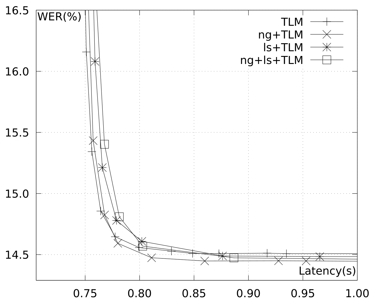
Figure 2 shows WER vs mean empirical latency figures, computed over
dev1-dev, with different pruning parameter values, and comparing the LM combinations including the Transformer LM. These measurements were made on an Intel i7-3820 CPU @ 3.60GHz, with 64GB of RAM and a GeForce RTX 2080 Ti GPU. On the one hand, we can see how combinations involving LSTM LMs are systematically shifted rightwards with respect to other combinations. This means that the LSTM LM has a clear negative impact on system latency, with little to no effect on system quality. This evidence corroborates our decision to remove the LSTM LM to define our contrastive system
c1-streaming_1500ms_nt. On the other hand, the TLM alone generally provides a good baseline that is slightly improved in terms of WER if we include the other LMs. However, this comes at the cost of increasing latency. Hence, we selected the Transformer LM in isolation for our final latency-focused streaming system. This system was our contrastive system no. 2, identified as
c2-streaming_600ms_t. Its empirical latency on
dev1-dev was 0.81 ± 0.09 s (mean ± stdev), and its performance was 12.3 and 16.9 WER points on
test-2018 and
test-2020, respectively. This is, with just a very small relative WER degradation of 6% with respect to the primary system, we got state-of-the-art (mean = 0.81 s) and very stable (stdev = 0.09 s) empirical latencies. This system has a baseline consumption (when idle) of 9 GB RAM and 3.5 GB GPU memory (on a single GPU), adding 256 MB RAM and one CPU thread per decoding (audio stream). For instance, decoding four simultaneous audio streams in a single machine would use four CPU threads, 10 GB RAM and 3.5 GB GPU memory.
Table 5 summarises the results obtained for all four participant ASR systems on the
dev2,
test-2018 and
test-2020 sets, and also includes the results obtained with our 2018 open-condition system for comparison. On the one hand, surprisingly, the offline system is surpassed by the three streaming ones on
test-2020, by up to 1.1 absolute WER points (6% relative). We believe that this is caused, first, by the Gaussian mixture HMM-based VAD module producing false negatives (speech segments labelled as non-speech). As the non-speech model was trained with music and noise audio segments, and given the inherent limitations of Gaussian Mixture models, it is likely to misclassify speech passages with loud background music and noise (often present in TV programmes) as non-speech. Second, the Full Sequence Normalization technique might not be appropriate for some types of TV shows, as local acoustic condition changes become diluted in the full-sequence normalization, leading to somewhat inaccurate acoustic scores that can degrade system performance at that point. On the other hand, it is remarkable that our primary 2020 system significantly outperforms the 2018 winning system by 28% relative WER points on both
dev2 and
test-2018 (25% in the case of our latency-focused system
c2-streaming_600ms_t), and also works under strict streaming conditions.
All these streaming ASR systems can be easily put into production environments using our custom gRPC-based server-client infrastructure (
https://mllp.upv.es/git-pub/jjorge/MLLP_Streaming_API, accessed on 7 January 2022). Indeed, ASR systems comparable to
c2-streaming_600ms_t and
c1-streaming_1500ms_nt are already in production at our MLLP Transcription and Translation Platform (
https://ttp.mllp.upv.es/, accessed on 7 January 2022) for streaming and off-line processing, respectively. Both can be freely tested using our public APIs, accessible via the MLLP Platform.


 ,
, 


