Laplace Transform for Finite Element Analysis of Electromagnetic Interferences in Underground Metallic Structures

Abstract

A numerical methodology is proposed for the calculation of transient electromagnetic interference induced by overhead high-voltage power lines in metallic structures buried in soil—pipelines for oil or gas transportation. A series of 2D finite element simulations was employed to sample the harmonic response of a given geometry section. The numerical inverse Laplace transform of the results allowed obtaining the time domain evolution of the induced voltages and currents in the buried conductors, for any given condition of the power line.

1. Introduction

Metallic buried pipelines sharing the same corridor as AC power lines are subjected to AC interference, which is potentially harmful to personnel and equipment [1,2,3]. Some of the most critical conditions for the pipelines’ integrity are caused by transient phenomena, such as lightning or short circuits of the power lines [4,5]. In particular, lightning strikes may cause discharge currents up to hundreds of $\mathrm{k}\mathrm{A}$ for a duration of several microseconds [6]. In the last few decades, considerable efforts have been devoted to the numerical simulation of interference problems involving power lines and earth-return metallic conductors. The existing methodologies for the assessment of such phenomena are generally based either on transmission line theory [7,8,9,10,11] or a combination of finite element methodologies (FEMs) and circuital analysis [12,13,14,15,16]. In either case, however, fundamental requirements for such modeling tools include the capability of taking into account variations in the soil resistivity [17,18], non-parallel pipeline–power line routings [19], and the presence of multiple metallic conductors, such as mitigation wires [20]. Finally, the majority of the currently employed numerical techniques are developed under the assumption of a sinusoidal steady-state [21,22,23]. Indeed, since the 2D FEM simulations of this kind of physical configuration require meshes that are both large and detailed [19], the adoption of time-marching procedures would result in substantial computational loads. In this work, a new methodology was developed for the FEM simulation of interference problems in transient conditions. The technique is based on a finite element analysis of the Laplace-transformed problem. Once the problem was solved in the Laplace domain for a set of complex frequencies, a numerical inversion technique was adopted to compute the time-response at any required time-instant. Unlike time-marching procedures, whose accuracy at a given instant depends on the previous ones, the Laplace transformation of the mathematical problem allows avoiding the dependence on the previous time steps [24]. Moreover, since the solution corresponding to each complex frequency in the Laplace domain is independent of the others, the proposed method easily lends itself to parallel implementations in high-performance computing facilities.

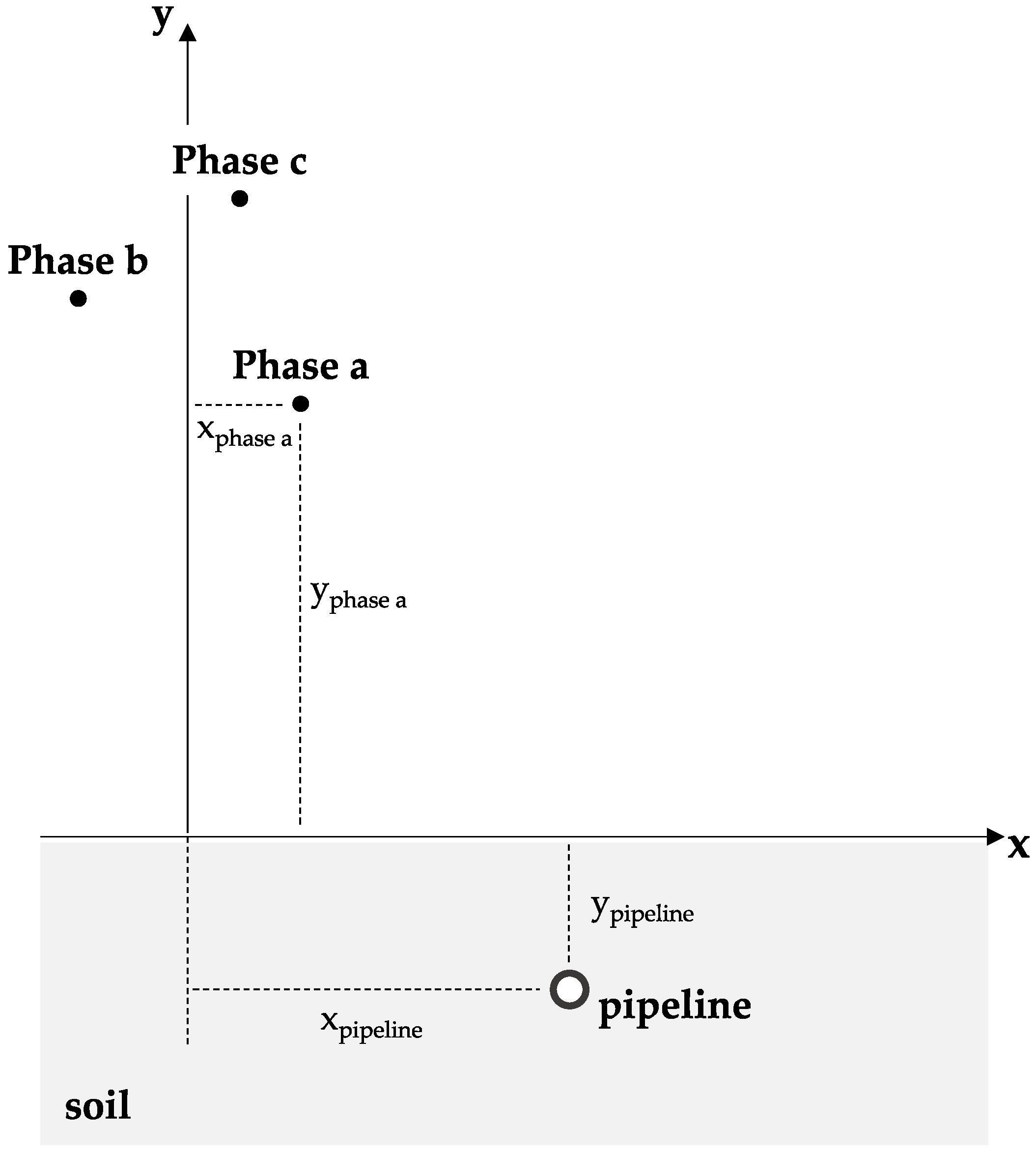
2. Model Formulation

The methodology described in this paper is based on a magnetoquasistatic formulation (i.e., ${\displaystyle \frac{\partial \mathrm{D}}{\partial t}}=0$) of the physical problem. The formulation holds if the condition $\sigma \gg (2\pi /\tau )ϵ$ is verified for the modeled conductors, where $\sigma$ and $ϵ$ are the electrical conductivity and permittivity, respectively, and $\tau$ the characteristic time of the considered electrical phenomena. The current densities and the magnetic vector potential were assumed to have a preferential direction, i.e., z. Hence, these can be defined as $\mathrm{J}=J_z\widehat{\mathrm{k}}$ and $\mathrm{A}=A_z\widehat{\mathrm{k}}$. By neglecting the spatial derivatives $\frac{\partial ·}{\partial z}$ of J and A along z, the problem can be formulated in the two-dimensional plane perpendicular to z. The governing equation is:

$$-\nabla ·(\frac{1}{\mu }\nabla A_z)+\sigma \frac{\partial A_z}{\partial t}=J_{0,z},$$

(1)

where $\mu$ is the magnetic permeability. The system’s forcing term $J_{0,z}=-\sigma \Delta {\phi }^{\prime }$ can be regarded as the current density that would flow in the conductors in the absence of the electromagnetic induction mechanism as a response to a per-unit length voltage $\Delta {\phi }^{\prime }$ applied along z.

Assuming that all materials behave linearly, a Laplace transform can be applied to Equation (1) to obtain a differential equation in the complex frequency s domain:

$$-\nabla ·(\frac{1}{\mu }\nabla {\tilde{A}}_z)+s\sigma {\tilde{A}}_z={\tilde{J}}_{0,z}+\sigma A_z\left(0^{-}\right).$$

(2)

Equation (2) is discretized by means of an FEM approach. The unknown is approximated by means of a piecewise polynomial representation ${\tilde{A}}_z(x,y)=\left\{N\right\}\left\{{\tilde{A}}_z\right\}$, where $\left\{N\right\}$ is the set of shape functions and $\left\{{\tilde{A}}_z\right\}$ is an array constituted by the nodal values of ${\tilde{A}}_z$. Using the generic shape function $N_k$ as the weighting function, the weak formulation resulting from Equation (2) is obtained from the weighted residual on the calculation domain $\mathrm{\Omega }$ bounded by the closed curve $\partial \mathrm{\Omega }$:

$${\int }_{\mathrm{\Omega }}\nabla N_k·(\frac{1}{\mu }\nabla {\tilde{A}}_z)\mathrm{d}S+s{\int }_{\mathrm{\Omega }}{N}_k\sigma {\tilde{A}}_z\mathrm{d}S={\int }_{\mathrm{\Omega }}{N}_k{\tilde{J}}_{0,z}\mathrm{d}S+{\int }_{\mathrm{\Omega }}{N}_k\sigma A_z\left(0^{-}\right)\mathrm{d}S+{\oint }_{\partial \mathrm{\Omega }}{N}_k\frac{1}{\mu }\frac{\partial {\tilde{A}}_z}{\partial n}\mathrm{d}l.$$

(3)

From Equation (3), a complex linear system is derived:

$$\left[\mathrm{K}\left(s\right)\right]\left\{{\tilde{A}}_z\right\}=RHS\left[{\tilde{J}}_{0,z},A_z\left(0^{-}\right)\right].$$

(4)

The coefficient matrix $\left[K\right]$ in Equation (4) is a sparse complex matrix. The values of $\left[K\right]$ depend on the properties (i.e., electrical conductivity and magnetic permeability) of the materials and on the complex frequency s. The right-hand-side term $\left\{RHS\right\}$ is a function of the transformed imposed current densities ${\tilde{J}}_{0,z}$, the initial distribution $A_z\left(0^{-}\right)$ of the magnetic vector potential, and the boundary conditions. That is, for a given set of initial and boundary conditions, Equation (4) allows the distribution of the vector potential ${\tilde{A}}_z$ to be found at a generic complex frequency s as the response of a forcing term ${\tilde{J}}_{0,z}$. Once Equation (4) has been solved, the current density in the complex frequency domain can be computed as:

$${\tilde{J}}_z={\tilde{J}}_{0,z}-s\sigma {\tilde{A}}_z+\sigma A_z\left(0^{-}\right).$$

(5)

The electric current flowing through a conductor is then found by integrating the current density computed by means of Equation (5) over the conductor cross-section.

The Laplace inversion formula used to compute the behavior of the physical quantities of interest $f\left(t\right)$ (e.g., the pipeline current or voltage) in the time domain from $\tilde{f}\left(s\right)$, i.e., the corresponding quantity in the frequency domain, is:

$$f\left(t\right)=\frac{1}{2\pi j}{\int }_{\alpha -j\infty }^{\alpha +j\infty }\tilde{f}\left(s\right)e^{st}\mathrm{d}s,$$

(6)

with $t>0$ and, defining ${\alpha }_0$ as the abscissa of convergence, $\alpha >{\alpha }_0$. The numerical procedure for computing Equation (6) is obtained by discretizing the domain $\left[\alpha -j\infty ,\alpha +j\infty \right]$ with a step amplitude $\Delta \omega =\pi /T$ and integrating the expression by means of the trapezoidal rule. The resulting discrete expression for computing Equation (6) is:

$$f\left(t\right)=\frac{e^{\alpha t}}{T}\mathrm{Re}\{\frac{\tilde{f}\left(\alpha \right)}{2}+\sum _{k=1}^{\infty }\tilde{f}\left(\alpha +j\frac{k\pi }{T}\right)e^{j\frac{k\pi t}{T}}\},$$

(7)

with $0<t<T$. Equation (7) is affected by a discretization error due to the trapezoidal rule. An additional error is introduced when the infinite sum in Equation (7) is arrested at the Nth term. The inversion is computed using the algorithm described in [25]. While the abscissa of convergence ${\alpha }_0$ must be provided by the user (${\alpha }_0=0$ for this work), the values of the T and N parameters are computed internally in order to satisfy the tolerance required by the user. The actual value of $\alpha >{\alpha }_0$ is also computed internally, as a function of the time t at which the inverse transform has to be evaluated. The process is repeated for the set of complex frequencies s at which Equation (3) is solved. Further details on the implementation of the numerical inversion algorithm can be found in [26].

A particularly relevant piece of information that can be obtained with the proposed methodology is the impulse response of the system. The convolution of the impulse response allows the behavior of the considered system to be evaluated as a response to any forcing term $J_{0,z}\left(t\right)$, avoiding the need to Laplace transform the forcing term itself.

3. Simulation Results

In this section, the developed methodology was employed to study the transient response of a typical corridor including an overhead power line and a metallic pipeline, buried in the soil. While real corridors can feature complex routings [27,28], the pipeline was assumed to run parallel to the power line for the sake of simplicity. A cross-section of the considered pipeline–power line corridor is reported in Figure 1. The geometrical and electrical characteristics of the considered conductors are summarized in

Table 1. Geometrical and electrical data.

Conductor	x (m)	y (m)	Radius (m)	Conductivity (S m${}^{-1}$)
Phase a	3.5	12	1.5 × 10−2	3.5 × 107
Phase b	−3	14	1.5 × 10−2	3.5 × 107
Phase c	2.9	16	1.5 × 10−2	3.5 × 107
pipeline	2	−1.1	5 × 10−1	5.5 × 106
soil	-	-	6 × 102	0.01

. In order to assess the effects of the pipeline magnetic properties, a sensitivity analysis was performed by assuming three different values of relative magnetic permeability, i.e., ${\mu }_r=500$, ${\mu }_r=250$ and ${\mu }_r=1$. The pipeline was perfectly insulated from the surrounding soil, and its thickness was $1.5$ $\mathrm{c}$$\mathrm{m}$. The soil was represented as a hemicircular region, whose radius value was selected according to the criteria discussed in [18]. To simplify the calculation, a uniform soil electrical conductivity was considered, since this hypothesis does not compromise the validity of the proposed methodology. Because of the condition $\sigma \gg (2\pi /\tau )ϵ$, discussed in Section 2, the developed approach cannot be applied to high-resistivity soils in the presence of fast electrical transients. In the following paragraphs, the described configuration is assessed with the methodology described in Section 2. The study was performed by comparing the current response of Phase Conductor a, the soil, and the pipeline when three different voltage signals are applied to Phase a (see Table 1).

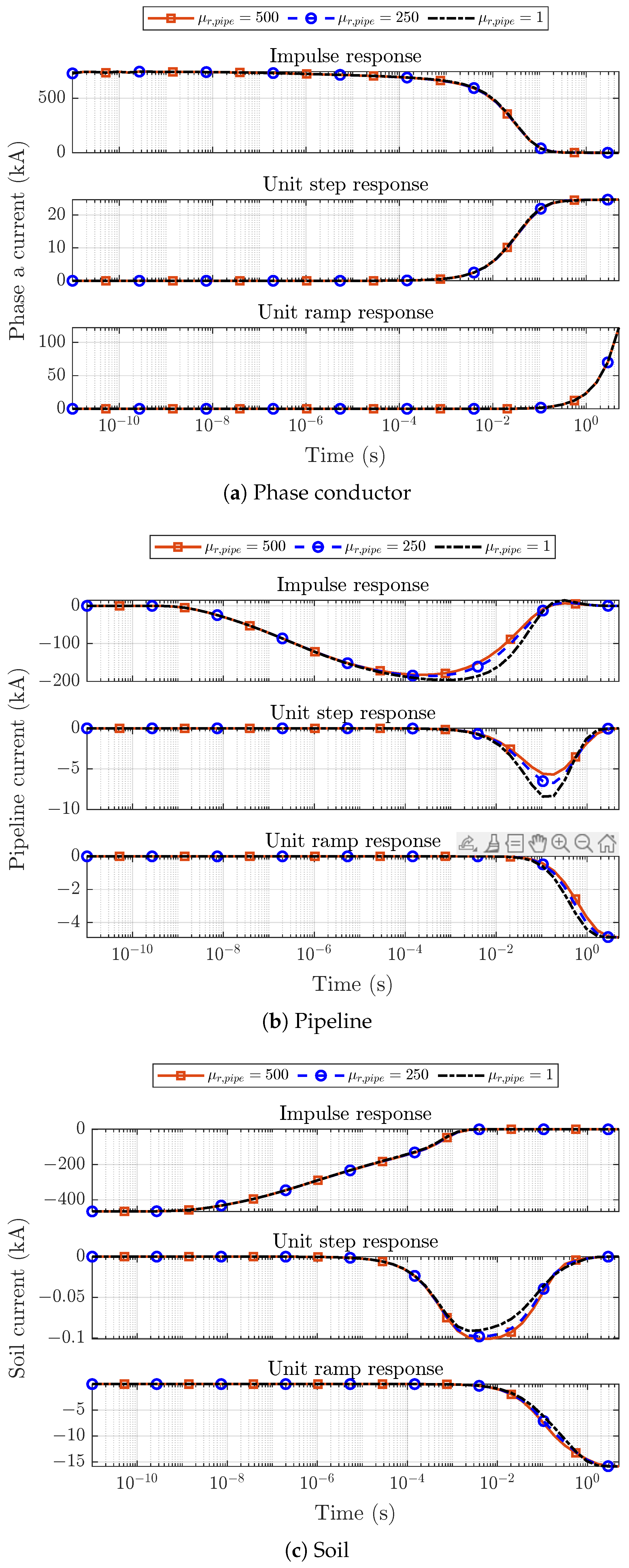
3.1. Time-Domain Current Response

Figure 2 shows the induced current in Phase Conductor a, the pipeline, and the soil when Phase Conductor a is subjected to three distinct $\Delta {\phi }^{\prime }$ per-unit length voltage waveforms. These are:

• Dirac impulse $\delta \left(t\right)\to \mathcal{L}\left(\delta \right)=1$;
• Unit step $u\left(t\right)\to \mathcal{L}\left(u\right)=\frac{1}{s}$;
• Unit ramp $r\left(t\right)\to \mathcal{L}\left(r\right)=\frac{1}{s^2}$.

3.1.1. Impulse Response

Figure 2a shows that, when subjected to a positive impulsive voltage $\delta \left(t\right)$, the phase conductor immediately responds with a current. Hence, the phase conductor current shows a discontinuity, due to the infinite power injected into the system by the impulsive voltage waveform. As can be observed in Figure 2b,c, the phase current impulse immediately induces a negative current in both the pipeline and the soil, due to Faraday’s law. Indeed, since the magnetoquasistatic approximation was adopted in the FEM model, the magnetic field instantaneously generated by the phase conductor propagates with infinite speed.

Due to the skin effect, an intense current density develops in the upper layers of the soil, screening the pipeline from the phase conductor magnetic field. This is the reason behind the observed delay in the pipeline current response with respect to the other conductors. The dynamics of the magnetic field diffusion in the soil are regulated by the product ${\mu }_s{\sigma }_s$, where ${\mu }_s$ and ${\sigma }_s$ are the soil’s magnetic permeability and electrical conductivity, respectively. Hence, defining d as the pipeline depth, $\left({\mu }_s{\sigma }_s\right)d^2$ yields a characteristic magnetic field penetration time ${\tau }_p=1.5\times {10}^{-8}$ s, compatible with the dynamics of the pipeline current in Figure 2b.

Focusing on the pipeline and soil impulsive response in Figure 2b,c, the induced negative current becomes positive at $0.138$ $\mathrm{s}$ and $2.7$ $\mathrm{m}$$\mathrm{s}$, respectively. This effect was obtained because of the progressive decrease of the phase conductor current from its initial value caused by the impulsive voltage waveform.

3.1.2. Unit Step and Unit Ramp Response

As concerns the unit step $u\left(t\right)$ and ramp $r\left(t\right)$ response of Phase Conductor a, considerably slower dynamics were obtained with respect to the described current response to an impulsive waveform. The reason behind this different behavior lies in the finite power associated with $u\left(t\right)$ and $r\left(t\right)$, as opposed to $\delta \left(t\right)$. Indeed, in these latter cases, the phase conductor (and soil) currents are bound to the energy continuity principle. Their time-evolution is regulated by the conductors’ resistance and inductance values.

The discussed slower dynamics obtained for the Phase Conductor a current results in the observed lag of the pipeline and soil response with respect to the impulsive waveform case. While $\delta \left(t\right)$ yields a substantial lag between the soil and pipeline currents, the same feature cannot be observed when $u\left(t\right)$ and $r\left(t\right)$ are considered. This is due to the above-discussed magnetic field characteristic penetration time ${\tau }_p$, whose value becomes negligible with respect to the soil current dynamics when $u\left(t\right)$ and $r\left(t\right)$ are considered, respectively.

Finally, the previously discussed inversion of the pipeline and soil current is not observed when the unit step and unit ramp responses are considered. This is due to the nature of $u\left(t\right)$ and $r\left(t\right)$, which results in a monotonic phase conductor current. Furthermore, it can be noticed that both the pipeline and the soil unit ramp responses approach a constant value since the phase conductor current increases linearly due to the applied unit ramp voltage waveform $r\left(t\right)$.

3.1.3. Influence of the Pipeline Magnetic Permeability

As can be noticed in Figure 2a, the different values of the pipeline relative magnetic permeability ${\mu }_r$ have a negligible influence on the phase conductor current. Conversely, higher values of ${\mu }_r$ lead to lower induced current magnitudes on the pipeline, shown in Figure 2b. This is because the pipeline penetration depth for the current density decreases with ${\mu }_r$, increasing the pipeline impedance. Finally, an opposite trend can be noticed for the unit step and unit ramp current response of the soil in Figure 2c, where the soil current magnitude increases with ${\mu }_r$. The soil current is caused by the opposite inductive contributions generated by the power line and the pipeline currents. Hence, since the power line current is substantially unaffected by ${\mu }_r$, when the pipeline current magnitude decreases, a larger current magnitude is induced in the soil.

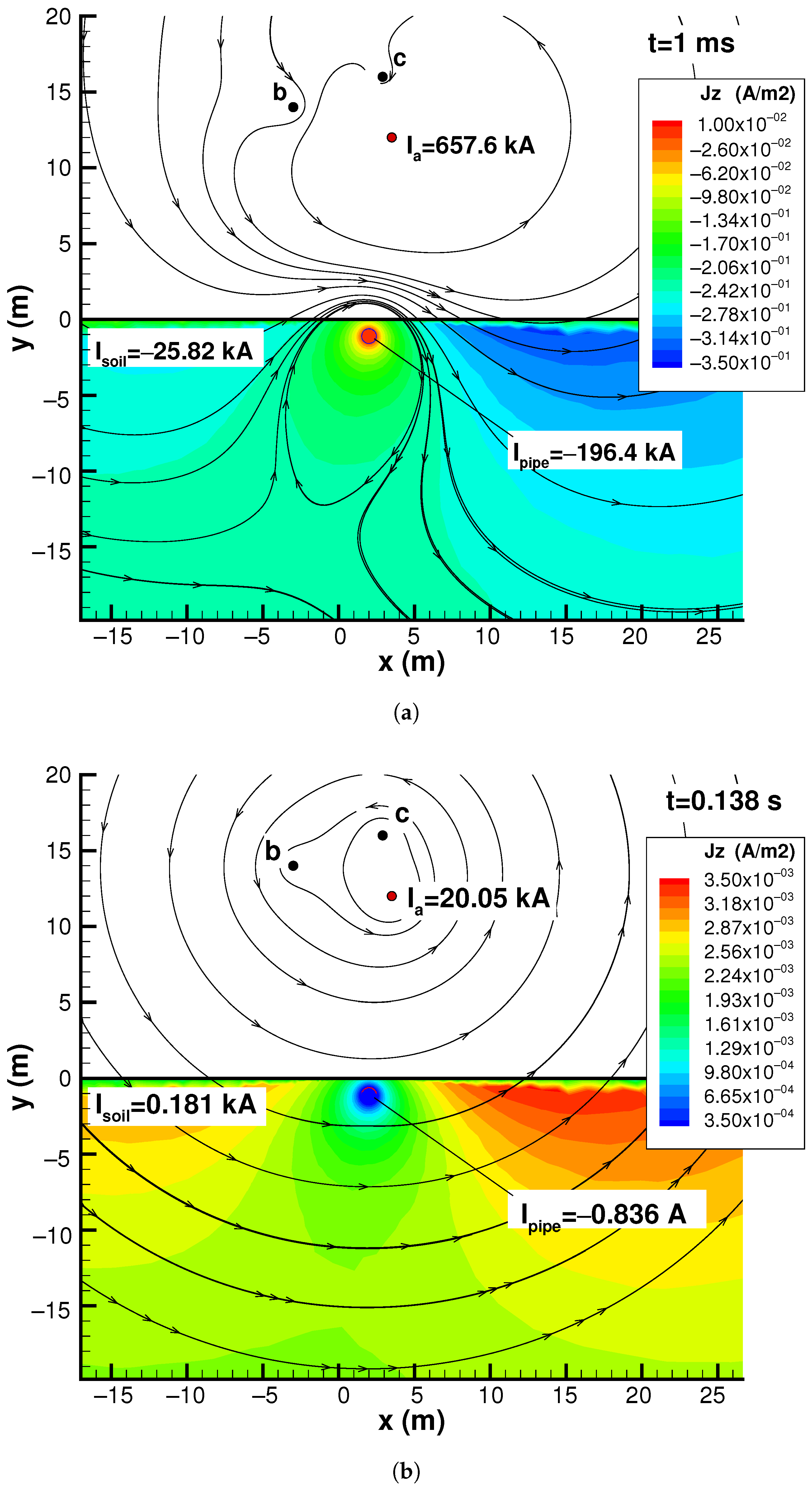
3.2. Time-Domain Current Density and Magnetic Flux Density Field

Figure 3 shows the soil current density and the magnetic field lines resulting from the application of a Dirac voltage impulse $\delta \left(t\right)$ to Phase Conductor a. The results in Figure 3a,b refer to two different instants of the same simulation and were obtained through the described numerical inversion of the solution in the Laplace domain.

Figure 3a shows the results after $1\times {10}^{-3}$ $\mathrm{s}$ from the application of the impulse. Comparing the obtained magnitudes of the phase conductor ($I_{phasea}$) and soil ($I_{soil}$) currents, $I_{soil}$ exhibits a faster decay. The soil features a lower time constant $\tau$ compared to the phase conductor, due to its lower electrical conductivity.

Finally, Figure 3b refers to $t=0.138\mathrm{s}$, i.e., the moment corresponding to the pipeline current sign inversion. This feature is highlighted by the change in magnetic field topology compared to Figure 3a.

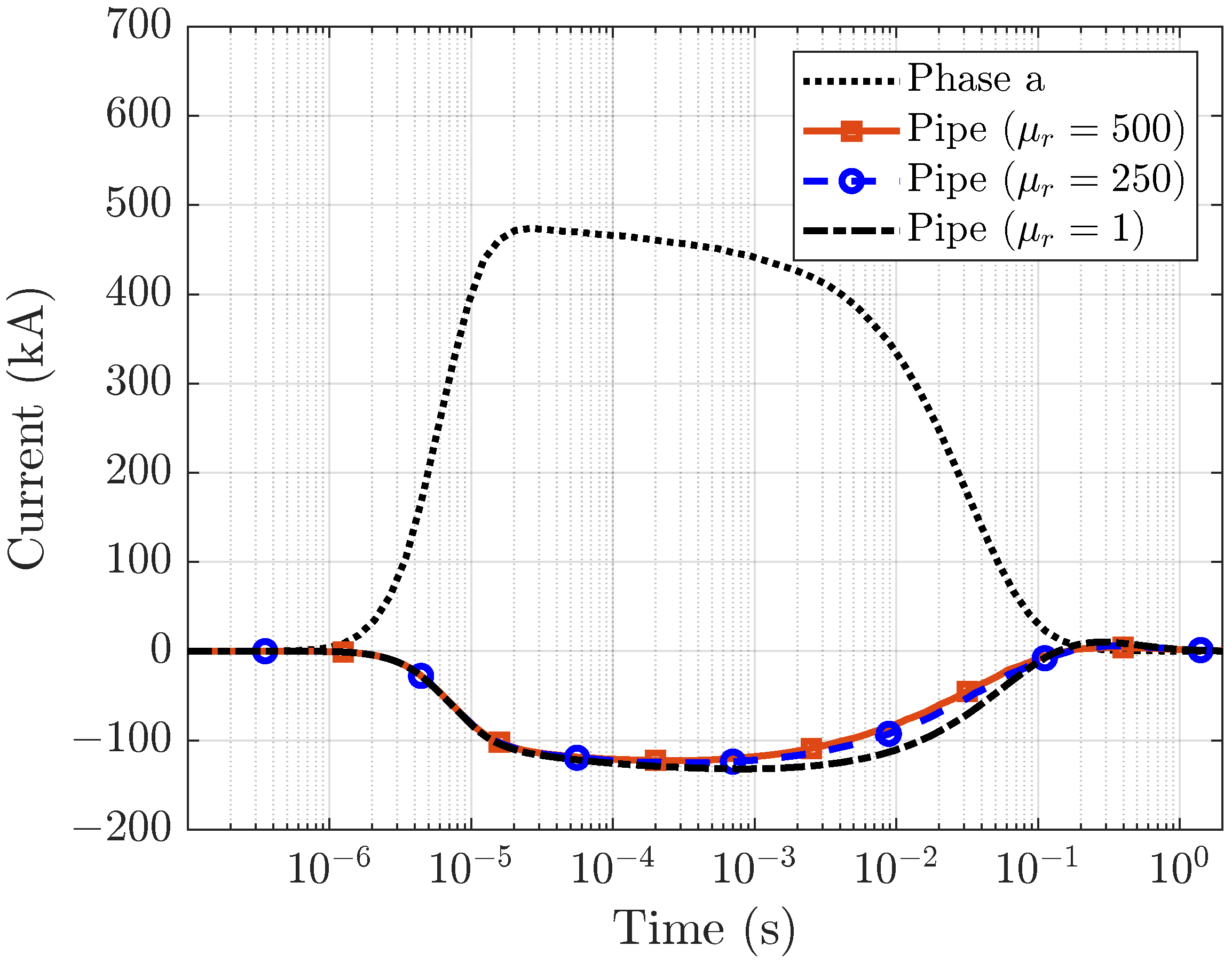
3.3. Pipeline Response to a Lightning Event Striking a Power Line Conductor

Once the impulse response of the conductors of a given system is available, it can be used to obtain the transient response to any given applied waveform. Let us consider the following physical situation: a lightning event striking Phase Conductor a of the power line described in Figure 1 and Table 1 of the previous section. The resulting voltage waveform on the phase conductor $\Delta {\phi }_L^{\prime }$ is shown in Figure 4. The applied per-unit length voltage $\Delta {\phi }_L^{\prime }$ was taken from the measurements performed by Piantini and Janiszewski on a scaled power line in [29]. The phase conductor current due to the lightning strike, $I_{phasea}$, can be obtained with the following convolution integral:

$$I_{phasea}\left(t\right)={\int }_{-\infty }^{\infty }\Delta {\phi }_L^{\prime }(t-\tau )I_{phasea,\delta }^{\prime }(\tau )\mathrm{d}\tau ,$$

(8)

where $I_{phasea,\delta }$ is the current impulse response of Phase Conductor a. Analogously, the transient pipeline current response to the lightning event can be obtained using $I_{pipeline,\delta }^{\prime }$, i.e., the impulse response of the buried pipeline:

$$i_{pipeline}\left(t\right)={\int }_{-\infty }^{\infty }\Delta {\phi }_L^{\prime }(t-\tau )I_{pipeline,\delta }^{\prime }\left(\tau \right)\mathrm{d}\tau .$$

(9)

It is worth noticing that $I_{phasea}^{\prime }$ and $I_{pipeline,\delta }^{\prime }$ in the two former expression have units of $\mathrm{A}\mathrm{m}{\mathrm{V}}^{-1}{\mathrm{s}}^{-1}$, since they were obtained as the response to a per-unit length voltage impulse with a time-integral equal to one. The computed currents on the pipeline and on Phase Conductor a are shown in Figure 5.

4. Conclusions

A numerical methodology was proposed and discussed for the assessment of electromagnetic interference induced by power lines in conductors buried in soil. The technique, based on the finite element solution in the Laplace domain and subsequent numerical inversion, allows taking into account the effects of arbitrary power line voltage and currents. The proposed method was used to derive the electrical response of a typical right-of-way to three different elementary waveforms, including a Dirac voltage impulse. Finally, the pipeline current induced by a lightning event striking the power line was obtained through the convolution of the previously computed impulse response and a lightning-induced voltage measurement. Future developments will focus on extending the methodology to study more complex and realistic cases, such as long and non-straight pipeline paths. This will be performed by applying the developed approach to multiple 2D sections of the geometry. The addition of suitable impedance networks will allow taking into account physical phenomena causing flows of current in the $xy$ (transverse) plane, such as currents due to an imperfect pipeline coating or capacitive effects. An adequate treatment of the latter is of fundamental importance to investigate propagation effects in electrically long structures. It is worth noticing that the proposed methodology can also be extended to account for a frequency-dependent magnetic permeability in a straightforward way. This can be achieved by selecting the permeability corresponding to the given value of the complex variable s when solving the problem in the frequency domain. This is an advantage compared to time-marching procedures, where one would have to deal with the challenge of identifying ${\mu }_r\left(f^{*}\right)$ corresponding to the given time instant $t^{*}$. On the other side, time-marching procedures would allow for a more straightforward modeling of the ferromagnetic nonlinear properties. Nevertheless, the use of Volterra series allows the applicability of the Laplace transform to be extended to nonlinear systems [30,31].

References

1. CIGRE. Guide on the Influence of High Voltage AC Power Systems on Metallic Pipelines; Technical Report, Cigré Working Group 36.02; CIGRE: Paris, France, 1995. [Google Scholar]
2. Baete, C.; Haynes, G.; Marmillo, J. Unmasking AC Threats on Petrochemical Pipelines. In Proceedings of the NACE CORROSION, Virtual, 19–30 April 2021. [Google Scholar]
3. Fieltsch, W.; Shahinas, F.; Olesen, A.J.; Nielsen, L.V. AC Corrosion at Other Frequencies Part A: Field Investigation and Mitigation. In Proceedings of the NACE CORROSION, Virtual, 19–30 April 2021. [Google Scholar]
4. Cotton, I.; Kopsidas, K.; Zhang, Y. Comparison of Transient and Power Frequency-Induced Voltages on a Pipeline Parallel to an Overhead Transmission Line. IEEE Trans. Power Deliv. 2007, 22, 1706–1714. [Google Scholar] [CrossRef]
5. Wu, X.; Zhang, H.; Karady, G.G. Transient analysis of inductive induced voltage between power line and nearby pipeline. Int. J. Electr. Power Energy Syst. 2017, 84, 47–54. [Google Scholar] [CrossRef]
6. Tleis, N. Power Systems Modelling and Fault Analysis: Theory and Practice; Elsevier: Amsterdam, The Netherlands, 2007. [Google Scholar]
7. Haubrich, H.J.; Flechner, B.A.; Machczynski, W. A universal model for the computation of the electromagnetic interference on earth return circuits. IEEE Trans. Power Deliv. 1994, 9, 1593–1599. [Google Scholar] [CrossRef]
8. Dabkowski, J. How to predict and mitigate A.C. Voltages on buried pipelines. Pipeline Gas J. 1979, 206, 19–21. [Google Scholar]
9. Dawalibi, F.P.; Southey, R.D. Analysis of electrical interference from power lines to gas pipelines. I. Computation methods. IEEE Trans. Power Deliv. 1989, 4, 1840–1846. [Google Scholar] [CrossRef]
10. Li, L.; Gao, X. AC corrosion interference of buried long distance pipeline. In Proceedings of the 2021 3rd International Conference on Intelligent Control, Measurement and Signal Processing and Intelligent Oil Field (ICMSP), Xi’an, China, 23–25 July 2021; pp. 342–346. [Google Scholar] [CrossRef]
11. Muresan, A.; Papadopoulos, T.A.; Czumbil, L.; Chrysochos, A.I.; Farkas, T.; Chioran, D. Numerical Modeling Assessment of Electromagnetic Interference Between Power Lines and Metallic Pipelines: A Case Study. In Proceedings of the 2021 9th International Conference on Modern Power Systems (MPS), Cluj-Napoca, Romania, 16–17 June 2021; pp. 1–6. [Google Scholar]
12. Cristofolini, A.; Popoli, A.; Sandrolini, L. Numerical Modelling of Interference from AC Power Lines on Buried Metallic Pipelines in Presence of Mitigation Wires. In Proceedings of the 2018 IEEE International Conference on Environment and Electrical Engineering and 2018 IEEE Industrial and Commercial Power Systems Europe (EEEIC/I&CPS Europe), Palermo, Italy, 12–15 June 2018; pp. 1–6. [Google Scholar] [CrossRef]
13. Micu, D.D.; Christoforidis, G.C.; Czumbil, L. AC interference on pipelines due to double circuit power lines: A detailed study. Electr. Power Syst. Res. 2013, 103, 1–8. [Google Scholar] [CrossRef]
14. Christoforidis, G.C.; Labridis, D.P.; Dokopoulos, P.S. Ahybrid method for calculating the inductive interference caused by faulted power lines to nearby buried pipelines. IEEE Trans. Power Deliv. 2005, 20, 1465–1473. [Google Scholar] [CrossRef]
15. Dawalibi, F.P.; Donoso, F. Integrated analysis software for grounding, EMF, and EMI. IEEE Comput. Appl. Power 1993, 6, 19–24. [Google Scholar] [CrossRef]
16. Abdullah, N. HVAC interference assessment on a buried gas pipeline. IOP Conf. Ser. Earth Environ. Sci. 2021, 704, 012009. [Google Scholar] [CrossRef]
17. Nakagawa, M.; Ametani, A.; Iwamoto, K. Further studies on wave propagation in overhead lines with earth return: Impedance of stratified earth. Proc. Inst. Electr. Eng. 1973, 12, 1521–1528. [Google Scholar] [CrossRef]
18. Popoli, A.; Sandrolini, L.; Cristofolini, A. Inductive coupling on metallic pipelines: Effects of a nonuniform soil resistivity along a pipeline-power line corridor. Electr. Power Syst. Res. 2020, 189, 106621. [Google Scholar] [CrossRef]
19. Popoli, A.; Sandrolini, L.; Cristofolini, A. Finite Element Analysis of Mitigation Measures for AC Interference on Buried Pipelines. In Proceedings of the 2019 IEEE International Conference on Environment and Electrical Engineering and 2019 IEEE Industrial and Commercial Power Systems Europe (EEEIC/I CPS Europe), Genova, Italy, 11–14 June 2019; pp. 1–5. [Google Scholar] [CrossRef]
20. Popoli, A.; Sandrolini, L.; Cristofolini, A. Comparison of screening configurations for the mitigation of voltages and currents induced on pipelines by HVAC power lines. Energies 2021, 14, 3855. [Google Scholar] [CrossRef]
21. Lucca, G. Mutual impedance between an overhead and a buried line with earth return. In Proceedings of the Ninth International Conference on Electromagnetic Compatibility, Manchester, UK, 5–7 September 1994; pp. 80–86. [Google Scholar]
22. Lucca, G. AC interference from a faulty power line on nearby buried pipelines: Influence of the surface layer soil. IET Sci. Meas. Technol. 2019, 14, 225–232. [Google Scholar] [CrossRef]
23. Popoli, A.; Cristofolini, A.; Sandrolini, L.; Abe, B.; Jimoh, A. Assessment of AC interference caused by transmission lines on buried metallic pipelines using F.E.M. In Proceedings of the 2017 International Applied Computational Electromagnetics Society Symposium—Italy, ACES 2017, Firenze, Italy, 26–30 March 2017; pp. 1–2. [Google Scholar] [CrossRef]
24. Conte, S.D.; Carl, W. De Boor, Elementary Numerical Analysis: An Algorithmic Approach; SIAM: Philadelphia, PA, USA, 2018. [Google Scholar]
25. D’amore, L.; Laccetti, G.; Murli, A. Algorithm 796: A Fortran software package for the numerical inversion of the Laplace transform based on a Fourier series method. ACM Trans. Math. Softw. (TOMS) 1999, 25, 306–315. [Google Scholar] [CrossRef]
26. D’amore, L.; Laccetti, G.; Murli, A. An implementation of a Fourier series method for the numerical inversion of the Laplace transform. ACM Trans. Math. Softw. (TOMS) 1999, 25, 279–305. [Google Scholar] [CrossRef]
27. Martins-Britto, A.G.; Moraes, C.M.; Lopes, F.V. Inductive interferences between a 500 kV power line and a pipeline with a complex approximation layout and multilayered soil. Electr. Power Syst. Res. 2021, 196, 107265. [Google Scholar] [CrossRef]
28. Martins-Britto, A.G.; Moraes, C.M.; Lopes, F.V. Transient electromagnetic interferences between a power line and a pipeline due to a lightning discharge: An EMTP-based approach. Electr. Power Syst. Res. 2021, 197, 107321. [Google Scholar] [CrossRef]
29. Piantini, A.; Janiszewski, J.M. Lightning-induced voltages on overhead lines—Application of the extended rusck model. IEEE Trans. Electromagn. Compat. 2009, 51, 548–558. [Google Scholar] [CrossRef]
30. Farina, A.; Bellini, A.; Armelloni, E. Non-linear convolution: A new approach for the auralization of distorting systems. In Proceedings of the Audio Engineering Society Convention 110, Amsterdam, The Netherlands, 12–15 May 2001. [Google Scholar]
31. Tronchin, L.; Coli, V.L. Further investigations in the emulation of nonlinear systems with Volterra series. J. Audio Eng. Soc. 2015, 63, 671–683. [Google Scholar] [CrossRef]
Figure 1. Cross-section of the considered pipeline–power line corridor. The physical characteristics of the conductors are reported in Table 1.
Applsci 12 00872 g001
Figure 2. Current response of Phase Conductor a (a), the pipeline (b), and the soil (c), as a result of different voltage waveforms enforced in Phase Conductor a at t = 0 s.
Applsci 12 00872 g002
Figure 3. Current density distribution and magnetic field lines at t   =   1   ×   10 3 s (a) and t = 0.138 s (b) obtained from the impulse response in the Laplace domain.
Applsci 12 00872 g003
Figure 4. Response of the phase conductor voltage to a lightning event from [29].
Applsci 12 00872 g004
Figure 5. Pipeline and Phase Conductor a current response to the lightning event shown in Figure 4.
Applsci 12 00872 g005