Abstract
Early detection of the dysfunction of the cardiac autonomic regulation (CAR) may help in reducing cannabis-related cardiovascular morbidities. The current study examined the occurrence of changes in the CAR activity that is associated with the consumption of bhang, a cannabis-based product. For this purpose, the heart rate variability (HRV) signals of 200 Indian male volunteers, who were categorized into cannabis consumers and non-consumers, were decomposed by Empirical Mode Decomposition (EMD), Discrete Wavelet transform (DWT), and Wavelet Packet Decomposition (WPD) at different levels. The entropy-based parameters were computed from all the decomposed signals. The statistical significance of the parameters was examined using the Mann–Whitney test and t-test. The results revealed a significant variation in the HRV signals among the two groups. Herein, we proposed the development of machine learning (ML) models for the automatic classification of cannabis consumers and non-consumers. The selection of suitable input parameters for the ML models was performed by employing weight-based parameter ranking and dimension reduction methods. The performance indices of the ML models were compared. The results recommended the Naïve Bayes (NB) model developed from WPD processing (level 8, db02 mother wavelet) of the HRV signals as the most suitable ML model for automatic identification of cannabis users.
1. Introduction
Cannabis is a dioecious annual plant, which is used to develop various therapeutic agents for the treatment of pain, nausea, and insomnia in cancer patients and anorexia in acquired immune deficiency syndrome (AIDS) patients [1]. However, the cannabis plant is also used to derive various recreational products like bhang, ganja, and charas. Cannabis-based recreational products are believed to have low toxicity, and their consumption is increasing day by day [2]. As per the reported literature, cannabis has become the most highly used psychotropic recreational compound across the globe, following alcohol and tobacco [1]. Many states of the USA have legalized the non-medical use of cannabis and have allowed companies to sell cannabis to adults who are older than 21 years old [3]. However, many recent reports have revealed the occurrence of a variety of unfavorable health effects of cannabis, including cardiovascular diseases [4]. Hence, it is important to identify the effect of cannabis intake on the cardiovascular activities of cannabis users. It is a well-known fact that the modulation in cardiac autonomic regulation (CAR) provides prognostic information about cardiovascular diseases [5]. This is attributed to the innervations of the sympathetic and vagal nerves of the ANS to the heart [6]. The functioning of the ANS can be understood non-invasively by analyzing the RR interval/HRV signals, derived from the electrocardiogram (ECG) signals [7]. Researchers have proposed both linear and nonlinear techniques for the processing of the HRV signals [8]. However, decomposition-based methods (e.g., EMD, DWT, and WPD) are getting more attention from researchers nowadays because of the nonlinear and non-stationary behavior of the HRV signals [8,9,10].
The EMD technique is a popular nonlinear signal decomposition technique, which was first proposed by Huang et al. (1998) [11]. It divides the input signal into mono-component functions called intrinsic mode functions (IMFs) and simplifies the further processing of the signals [8]. Several researchers have proposed that subtle variations within the HRV signals can be identified easily using EMD [8]. Pachori et al. (2015) performed the EMD analysis of the HRV signals for the automated detection of diabetes [12]. The EMD-based decomposition of the HRV signals produced six IMFs. The IMFs were used to extract two time-domain parameters and three frequency-domain parameters [12]. The clinically significant variations were obtained between the diabetic and control groups, suggesting the applicability of the EMD method in the automated identification of diabetic patients. Djelaila et al. (2016) used EMD analysis of HRV signals and calculated the power spectral density (PSD) of the IMFs for the detection of cardiac arrhythmia [13]. Acharya et al. (2017) reported EMD-based processing of HRV signals to facilitate the automated detection of congestive heart failure (CHF) disease [8]. Each of the HRV signals was decomposed into six IMFs, and 13 types of entropies were extracted from them. The extracted parameters were ranked using five ranking methods, and the highly-rated variables were classified using probabilistic neural networks and support vector machines. The normal and the CHF classes could be classified with the accuracy, sensitivity, and specificity of 97.64%, 97.01%, and 98.24%, respectively. Thus, the authors recommended that the proposed automated method could be employed to recognize the persons suffering from CHF, which will help the clinicians to plan their treatment.
In the last few decades, studies have also been carried out on wavelet (DWT and WPD)-based decomposition of the HRV signals [14,15]. The DWT represents a widely used wavelet-based decomposition method that simultaneously enables the time and frequency domain analyses of the signals [16]. Acharya et al. (2015) employed DWT-based processing of HRV signals for automated diagnosis of diabetes [10]. The HRV signals were extracted from 30 volunteers (15 controls and 15 diabetics). The decomposition of the HRV signals was performed using DWT (level 5, db08 mother wavelet). The parameters, namely, energy, sample entropy, approximation entropy, kurtosis, and skewness, were extracted from the wavelet coefficients, and the ranking of the parameters was carried out. The classification of diabetic and control groups could be performed with a maximum accuracy of 92.02% using the decision tree (DT) algorithm. Thus, the authors recommended that DWT can be considered as a potential candidate for the processing of the HRV signals. The WPD technique represents an extension of the DWT technique. It decomposes a signal like that of DWT. However, the difference lies in the fact that both the approximation and the detail coefficients of WPD participate in decomposition, unlike DWT, where only the approximate coefficient is decomposed at each level. Suparerk Janjarasjitt (2017) proposed WPD (level 3, db02 mother wavelet)-based processing of HRV data for detecting congestive heart failure (CHF) [15]. The spectral exponent of the HRV data was computed and the author could correctly discriminate the CHF patients from the people who were having a normal sinus rhythm. Therefore, WPD has been suggested as a potential method for the processing of the HRV signals. Recently, Geng et al. (2020) used WPD for the parameter extraction of HRV signals along with the Hilbert Huang Transform (HHT) and the Singular Value Decomposition (SVD) techniques for the development of an automatic sleep-staging decision support system [9]. The parameters extracted using WPD exhibited the highest classification accuracy for the random forest (RF) classifier suggesting the superiority of WPD compared to HHT and SVD methods of parameter extraction for HRV signals.
Although the above-mentioned nonlinear signal decomposition methods have been used by many researchers in the processing of HRV signals to carry out the detection of various diseases, no studies could be found that have implemented them for the detection of any alteration in the CAR due to cannabis consumption. Taking motivation from the above-mentioned facts, the current article proposes the decomposition of the HRV signals using the EMD, DWT, and WPD methods to identify variations in the CAR activity in a habitual bhang (a cannabis product)-consuming population. Furthermore, an ML-based model for automatic detection of cannabis users has also been designed. In this manuscript, bhang has been represented as cannabis unless otherwise mentioned.
2. Results
2.1. EMD-Based Analysis of the HRV Signals
EMD has been reported to be an efficient method for the processing of nonlinear and non-stationary data [8]. This may be attributed to its adaptive nature [11]. The HRV signals were subjected to EMD-based decomposition. The decomposition resulted in the generation of at least seven IMFs for each of the HRV signals. Hence, seven IMFs were considered for further analysis [12]. The typical IMFs for HRV signals belonging to Category-C and Category-B have been shown in Figure 1.
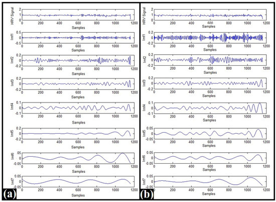
Figure 1.
Typical IMFs of 5 min HRV signals: (a) Category-C and (b) Category-B.
The extraction of 11 entropy-based parameters (described in Section 4.3) was carried out from each of the IMFs. The extracted parameters were named XY, where X represents the IMF name and Y indicates the base name of the parameter. Out of the 77 parameters extracted from 7 IMFs, 49 parameters were found to have non-normal distribution, and the remaining 28 parameters exhibited normal distribution as per the Shapiro–Wilk Test. The Mann–Whitney U test (with a critical p-value of 0.05) was used to analyze the statistical importance of the IMF parameters having non-Gaussian distribution. It revealed that the IMF7SpE parameter was significantly different (p-value ≤ 0.05) among Category-C and Category-B. The statistical importance testing using the t-test for the parameters having Gaussian distribution suggested four significantly different parameters among Category-C and Category-B. The statistically different parameters include IMF5SVDE, IMF5SpE, IMF5FI, and IMF5HjC. The median (MD) ± standard deviation (SD), and the25th and 75th percentile values of these parameters, have been tabulated in Table 1.

Table 1.
Characteristics of statistically important IMF-derived parameters.
Among all the extracted entropy-based parameters, the parameters that ranked within the top 10 by the weight-based parameter ranking methods and the parameters suggested by the dimensionality reduction methods were used as input for developing nine ML models as discussed in Section 4.5.2. As a result, 135 ML (9 ML models × 15 weight-based selection methods) models were developed from 15 weight-based parameter ranking methods, and 45 ML (9 ML models × 5 dimensionality reduction methods) models were obtained from 5 dimensionality reduction methods. The most accurate ML models (out of the nine ML models) along with their performance measures generated from each parameter selection method are shown in Table 2 [17].
Table 2.
Performance matrix of the machine learning models.
The GBT models generated using the ten important parameters obtained from the “Deviation” and “IG” parameter ranking methods exhibited an accuracy of 67.00 ± 10.06 and 67.00 ± 9.78%, respectively. Although the mean value of the accuracy was the same in both the models, the standard deviation (SD) of the IG-based GBT model was relatively lower than that of the Deviation-based GBT model. Hence, the IG-based GBT model was selected as the most suitable model for automatic identification of cannabis consumers using EMD-based processing of the HRV signals. The GBT model is an ensemble of either classification or regression trees, which uses boosting to provide the results with progressively improved estimations [18]. The proposed GBT model generated 20 classification trees to provide the final classification result. A typical classification tree among them has been shown in Figure 2.
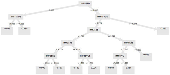
Figure 2.
A typical classification tree generated by the GBT Model.
2.2. DWT-Based Analysis of the HRV Signals
DWT is a popular joint time-frequency analysis method that helps to detect subtle variations in the signals [10]. The DWT-based decomposition of the HRV signals was performed from level 2 up to level 8 using Daubechies (db02, db04, db06, and db08) mother wavelets [10]. Hence, 28 different sets of DWT wavelet coefficients were generated in our study. The representative DWT coefficients generated for level 6 decomposition (using db02 mother wavelet) of HRV signals that belonged to Category-C and Category-B, respectively, have been shown in Figure 3.
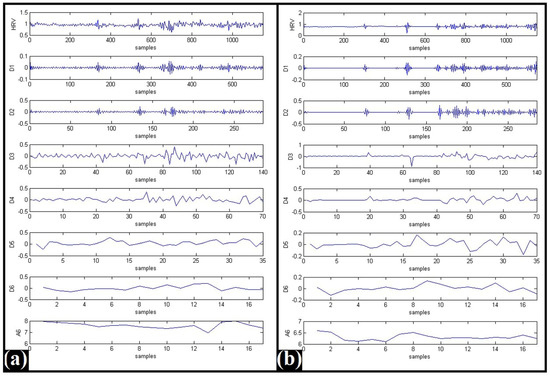
Figure 3.
Typical DWT coefficients for db02 mother wavelet-based level 6 decomposition of HRV signals: (a) Category-C and (b) Category-B.
A total of 11 entropy-based parameters were extracted from each wavelet coefficient. The extracted parameters were named as PQ, where P corresponded to the base name of the parameter and Q indicated the index of the wavelet coefficients. The index of the wavelet coefficients started from 0, i.e., the 1st wavelet coefficient was assigned with the index number 0. For each of the parameters extracted from the 28 different sets of DWT wavelet coefficients, the nature of distribution was found using the Shapiro–Wilk test. The results suggest that the majority of the parameters have non-Gaussian distribution, and the Mann–Whitney U test was performed to test their statistical significance. The parameters having Gaussian distribution were subjected to the t-test to examine their statistical importance. The MD ± SD, and the 25th and 75th percentile values of the statistically important parameters that were extracted from only db02 mother wavelet-based level 2 decomposition, have been provided in Table 3 as a typical representation.
Table 3.
Characteristics of statistically important parameters extracted from db02 mother wavelet-based level 2 decomposition of the HRV signals using DWT.
The parameters were examined for their relevance in the development of ML models using weight-based ranking and dimensionality reduction methods. In the case of the ranking methods, the parameters which ranked within the top 10 were considered relevant. The relevant parameters were used as inputs for the development of the ML models. The accuracies and AUCs of the most efficient ML models developed from the various levels of decomposition of the HRV signals have been provided in Table 4, [17]. The GBT model generated during level 8 decomposition (using db08 as the mother wavelet) exhibited the highest accuracy of 73.00 ± 5.87. The top 10 important parameters suggested by the “GI” parameter ranking method were used as the input parameters for the development of this GBT model.
Table 4.
Classification and AUC accuracies of the best ML models generated from DWT-based processing of HRV signals at different decomposition levels.
2.3. WPD-Based Analysis of the HRV Signals
The WPD method is a generalization of the DWT technique, where both the approximation and the detail coefficients participate in the decomposition process [19]. The HRV signals were subjected to WPD-based decomposition up to level 8 using Daubechies (db02, db04, db06, and db08) mother wavelets [10]. The typical WPD coefficients generated from level 2 decomposition of the HRV signals (using db02 mother wavelet) that belonged to Category-C and Category-B have been shown in Figure 4.
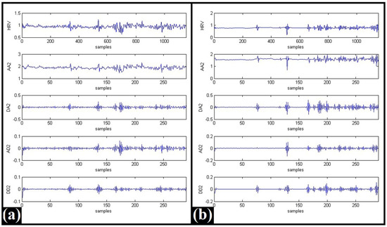
Figure 4.
Typical WPD coefficients for db02 mother wavelet-based level 2 decomposition of HRV signals: (a) Category-C, and (b) Category-B.
The extraction and naming of 11 entropy-based parameters were carried out from each of the WPD coefficients, which was similar to that of the DWT-based processing of HRV signals. The Shapiro-Wilk test revealed that majority of the parameters exhibited a non-normal behavior. Hence, their statistical importance was analyzed using the Mann–Whitney U test. The parameters that suggested normal behavior were analyzed for their statistical importance using the t-test. The results of the statistical test suggested several parameters varied significantly among Category-C and Category-B (p-value ≤ 0.05). The MD ± SD, and the 25th and 75th percentile values of the statistically important parameters extracted from db02 mother wavelet-based level 2 decomposition using WPD, have been provided in Table 5 as a typical representation.
Table 5.
Characteristics of statistically important parameters extracted from db02 mother wavelet-based level 2 decomposition of the HRV signals using WPD.
The judgment of the relevance of the parameters using ranking and dimensionality reduction methods as well as the development of the ML models was carried out similarly to that of DWT-based processing of the HRV signals. The accuracies and AUCs of the most efficient ML models developed from each decomposition level in WPD-based processing of the HRV signals have been provided in Table 6. The NB model generated during level 8 decomposition (db02 mother wavelet) exhibited the highest accuracy of 75.00 ± 13.94% among all the ML models that were developed using WPD-based processing of the HRV signals. This model used the top 10 important parameters ranked by the “SVM” method as the input parameters.
Table 6.
Classification and AUC accuracies of the best ML models generated from WPD-based processing of HRV signals at different decomposition levels.
3. Discussion
Cannabis refers to one of the ancient annual plants that are found mainly in Central Asia. It has been reported that cannabis plants were cultivated in China as much as 10,000 years ago for food and medical applications [20]. The ancient use of cannabis is also evident from the mythological scriptures. In Hindu mythology, cannabis (bhang) has been designated as the favorite food of Lord Shiva, and it is used as a beverage in many ceremonies like Shivaratri, Holi, etc. However, cannabis-based products are also consumed as popular illicit drugs due to their psychoactive behavior. In the last 50 years, the recreational intake of cannabis by adolescents and young adults has increased exponentially. As per Hall et al. (2009), the recreational cannabis intake by college students was first observed in 1979 in the USA, and it has gradually spread to the entire globe [21]. Cohen et al. (2019) have reported that ~4% of the entire population of the globe consume cannabis. Consumption is more in the USA compared to other rich countries in Europe [22]. The authors have revealed that ~11% of the US population have taken cannabis at least once in their lifetime. This might be because of the legalization of recreational cannabis use by adults in various states of the USA since 2012 [23]. However, various adverse health effects of recreational cannabis intake have been found in regular cannabis users [22]. This has been evident from the increased emergency department visits and hospitalizations by regular cannabis users. Among the various adverse health effects of cannabis consumption, the risk of addiction remains the primary concern [24]. It has both short-term as well as long-term influences on the functioning of the brain. The short-term effect depends on the way that cannabis is consumed. When a person smokes cannabis, the psychoactive compound (i.e., tetrahydrocannabinol (THC)) reaches the lungs directly, from where it quickly partitions into the bloodstream. The compound is then easily transported to the brain and other organs. On the other hand, THC is passed to the brain at a slower rate of up to 30 min to 1 h when it is consumed as a food or drink. The psychoactive compound acts on the brain cell receptors, thereby inducing short-term effects like altered sense, delusion, psychosis, and hallucination. The long-term effects of cannabis consumption on the brain include the decline in intelligence quocient (IQ) level and verbal ability, and the risk of anxiety and depression. The physical effects of cannabis on breathing, pregnancy, and vomiting, etc., have also been reported in addition to the mental effects.
The adverse effects of cannabis consumption on cardiovascular activities were also acknowledged more than four decades ago [25]. Some of the common and acute effects include an increment in heart rate and blood pressure that causes an enhancement in the workload of cardiac muscles. Kalla et al. analyzed the National Inpatient Sample (NIS) database of patients to understand the prevalence of cardiovascular diseases in people who regularly consumed cannabis [26]. They found that diseases like a cardiac failure and coronary artery disease were more in cannabis users than in the general population. Van Keer reported a case of complete heart block in a 19 year-old boy after the intake of cannabis [27]. The treatment of the patient was started using IV isoprenaline, and the occurrence of bradycardia was resolved within 24 h. Based on the outcomes, the boy was advised to stop consuming cannabis and the author recommended that the doctors in the emergency department should be aware of the potential cardiovascular effects of cannabis intake. Although many such cardiovascular complications have been reported in cannabis takers [4,28], the underlying mechanisms causing such effects are still very little known [25]. Hence, it is the need of the hour to understand the modulation in cardiovascular activity that is caused by cannabis consumption.
An understanding of the CAR provides valuable diagnostic information about the cardiovascular activity. This is because the rhythmic contraction of the heart is primarily regulated by the ANS through its nerve innervations (both vagal and sympathetic) into the heart. The ANS activity results in the alteration of the time duration between the consecutive RR intervals (also regarded as the HRV signals) [29]. Hence, the HRV signals have been widely used in the last few decades for diagnosing any imbalance in the CAR activity due to any external stimuli or diseases [8]. Usually, the processing of the HRV signals is performed using the time domain (statistical, geometric), frequency domain (e.g., FFT, AR), or the nonlinear methods (e.g., Poincare plot, recurrence quantification analysis (RQA), correlation dimension, and detrended fluctuation analysis (DFA)) [30]. However, several recent studies have proposed the use of signal decomposition-based techniques like EMD, DWT, and WPD for the analysis of the HRV signals [8,9,10]. This may be attributed to their ability to evaluate the original signatures that are present within the nonlinear and non-stationary HRV signals [8,31]. Hence, EMD, DWT, and WPD-based processing of the HRV signals were performed in the current study to examine the existence of any alteration in the CAR activity due to cannabis consumption. The EMD method resulted in the generation of at least seven IMFs from each HRV signal. Hence, only the first seven IMFs of each HRV signal were chosen as the input signals for the feature extraction process [12]. The selection of the appropriate mother wavelet plays a vital role in the wavelet analysis of the signals. Singh et al. (2006) have advocated the use of the Daubechies series of the mother wavelet for the processing of the HRV signals due to its ability to clearly reveal the properties of the transient and other components of the HRV signals [32]. Hence, Daubechies (db) wavelet was used as the mother wavelet for the processing of the HRV signals using DWT and WPD. The level of decomposition of the HRV signals was varied from 2 to 8 for identifying the most suitable level of decomposition.
The entropy-based parameters were extracted from the IMFs and the wavelet coefficients to obtain useful information related to the corresponding HRV signals. The reason behind the extraction of the entropy-based parameters may be attributed to the fact that entropy reveals the rate of generation of the information in a dynamical system and is extensively used as a complexity measure in the biomedical signal analysis [8,33]. Apart from this, the entropy-based parameters also help to quantify the degree of regularity in the signal by examining the repetitive patterns [34].
It is customary to use hypothesis testing as a tool for establishing whether there is a significant difference between the data of two populations using samples of a relatively lower size [35]. The t-test method was used for hypothesis testing when the parameter followed the normal distribution. However, most of the IMF and wavelet coefficient-derived entropy parameters did not exhibit the normal distribution (evident from the Shapiro—Wilk test). Hence, the Mann–Whitney U test (with a critical p-value = 0.05) was used to identify the significantly varying parameters for such parameters, which is a nonparametric statistical method. This method does not require the normal distribution of the parameters [36]. The results of the t-test and Mann–Whitney U test revealed many statistically significant parameters. This corresponds to the existence of variation in the characteristics of the HRV signals obtained from Category-C and Category-B. The variation in the HRV signal behavior might be due to the alteration in the CAR activity induced by cannabis intake. This is because HRV signals are regarded as a non-invasive indicator of CAR [37]. The analysis of these HRV signals using time and frequency methods by our group [38] has revealed an increase in sympathetic activity and a corresponding reduction in parasympathetic activity due to the regular intake of cannabis. This information further supported the hypothesis regarding the alteration of CAR activity due to the regular consumption of cannabis.
The ML models are currently extensively studied for the development of automated decision support systems for biomedical applications [39]. Many youths across the globe are getting addicted to cannabis products and may suffer from various health issues in the future. The development of automated cannabis user detection can help the healthcare givers to detect the changes in cardiac electrophysiology at an early stage. Accordingly, healthcare givers can counsel cannabis users to refrain from its consumption. Hence, the current study is an attempt to develop an ML model that can be used for the automated detection of the bhang-consuming population from their HRV signals. Although the efficiency of our developed ML models based on signal decomposition techniques may not be high, it will help researchers to do further research in this direction to develop robust automated cannabis-user detection systems that will contribute to the computer-aided prognosis of cannabis-induced ailments.
A small and efficient set of signal parameters is important for the development of an ML model [40]. This is because the optimal number of parameters reduces the complexity of the feature space that helps the model to achieve better performance. It also reduces the noise of the target signal [40]. Therefore, 15 weight-based parameter ranking methods and 5 dimensionality reduction methods were applied for the identification of the reduced set of the appropriate parameters to develop the ML models. The important parameters revealed by each method were used to train and validate nine ML models. The most accurate models developed from the EMD, DWT, and WPD decomposition methods have been summarized in Table 2, Table 4 and Table 6, respectively. The accuracy (75.00 ± 13.94%) of the NB model generated from the WPD-based processing of the HRV signals outperformed the highest accuracies of the best GBT models, i.e., 73.00 ± 5.87% and 67.00 ± 9.78%, generated by the DWT and EMD-based processing of the HRV signals, respectively. The other performance measures for this model were the AUC of 0.797 ± 0.130, precision (%) of 76.66 ± 15.22%, the F-measure (%) of 73.90 ± 15.22%, sensitivity (%) of 72.00 ± 16.87%, and specificity (%) of 78.00 ± 13.98%. Most of these measures were also superior to the other models. Hence, the NB model generated from WPD-based decomposition (db02 mother wavelet) of HRV signals at level 8 has been proposed for the automated identification of the bhang consuming population.
An in-depth review of the recent literature on the effects of cannabis on cardiovascular health was conducted. A comparative analysis of the studies has been summarized below in Table 7.
Table 7.
Recent studies on the effects of cannabis on cardiovascular health.
4. Materials and Methods
4.1. Acquisition of the ECG Signals and Extraction of the HRV Signals
The present study involved the analysis of the HRV signals of 200 paddy-field workers who had given consent to volunteer in this study. All of them were residents of the Sambalpur district in Odisha, India [38]. Written consent from the volunteers was taken as per the World Health Organization (WHO) guidelines. Initially, there were 218 paddy-field workers, out of which 207 paddy-field workers gave written permission for their voluntary participation in the study after detailed information about the study was provided to them. Out of the 207 interested volunteers, 200 volunteers were chosen for this study based on our inclusion criteria of 18–60 years of age and no occurrence of cardiovascular diseases [38]. Prior ethical approval was received from the Institute Ethical Committee (IEC) of NIT Rourkela, India (Ref.# NIRTKL/IEC/FORM-2/002; dated 16/8/2017) to acquire the ECG signals. The ECG signals were acquired using an ECG machine (VESTA 121i ECG machine, RMS Pvt. Ltd., India) for 5 min in the lead-I configuration. The sampling rate of the ECG machine was 500.6 Hz. The acquired signals were divided into two categories, i.e., Category-C (control group) and Category-B (bhang consuming group) [38]. Each of the categories comprised 100 signals. The ECG signals were processed through the Biomedical Workbench toolkit of LabVIEW (V2017, National Instruments, USA) and were further analyzed using the Pan–Tompkins algorithm to extract the RR interval signals (also known as HRV Signals). The ECG Feature Extractor tool of the Biomedical Workbench toolkit initially performs the signal enhancement through bandpass filtering (10–25 Hz). The employment of the bandpass filter allows for the extraction of the QRS complexes from the ECG signals. After the filtering process, the processed signal is rectified by squaring the signal. The combined processing technique allows the ECG Feature Extractor tool to extract the R waves accurately [46]. The use of default settings has also been suggested in numerous studies like Zaidi et al. (2017) [47] and Khong et al. (2019) [48]. The tool subsequently uses a threshold adjustment factor for the identification of the R peaks. In other words, a threshold value is used to detect the peak of the R-wave. The default threshold adjustment factor of 0.1 was used in our study. Furthermore, the “remove noise from raw signal” box was ticked to obtain a noise-free measurement, as recommended by Khong et al. (2019) [48]. The HRV signals were resampled at 4 Hz before subjecting them to decomposition using the EMD, DWT, and WPD methods [49].
4.2. Decomposition of the HRV Signals
4.2.1. EMD
The decomposition of the signals using EMD is a relatively new nonlinear signal processing method. It is employed for the processing of nonlinear and non-stationary signals [11]. Herein, the basis functions for decomposition are derived from the signal itself, unlike the Fourier or wavelet transforms where the basis signal is pre-fixed. The EMD method decomposes a given signal into several intrinsic mode functions (IMFs) and a residue (Equation (1)) using the process regarded as sifting [50]. The IMFs are a set of amplitude and frequency (AM–FM) modulated signal components. They satisfy two criteria: (i) the number of maxima and minima should be either the same or vary only by one to the number of zero crossings, and (ii) the average value of the envelopes formed by connecting local maxima and minima of the signal is zero [8]. As the HRV signals are nonlinear and non-stationary [38], the decomposition of the HRV signals was carried out by EMD. The implementation of the decomposition process was carried out in MATLAB software (2015a, MathWorks Inc., Natick, MA, USA).
where M represents the number of IMFs, fk(t) indicates the kth IMF, and rM corresponds to the residue.
4.2.2. DWT
The DWT is a widely used joint time-frequency analysis method [16]. Herein, the term wavelet refers to irregular, non-symmetric, and short-duration waveforms having finite energy, zero mean, and a real value of Fourier transform [19]. Wavelets have been used to analyze typical events that are embedded within a signal. Researchers have used DWT as an efficient tool for the processing of non-stationary signals. In DWT, the signals are decomposed into the detail and the approximation coefficients at each level by passing them through a high-pass and a low-pass filter, respectively. The detail coefficient is kept undivided, but the approximation coefficient is subjected to decomposition again in the next step, which results in the formation of a new set of detail and approximation coefficients. The decomposition process continues till the desired level of decomposition has arrived. Hence, a signal x(t) can be expressed as the sum of its approximation coefficient at a specific scale m0 (i.e., xm0(t)) and the detail coefficients with scales ranging from − to m0 as shown in Equation (2) [51]. The decomposition of the HRV signals using DWT was carried out in this study with the help of MATLAB software (2015a, MathWorks Inc., Natick, MA, USA).
where, xm0(t) = approximation coefficient at scale m0 and dm(t) = detail coefficient at scale m.
4.2.3. WPD
The WPD method is an extension of the DWT method with the advantage of providing a more precise decomposition of the high-frequency components of the given signal [52]. It differs from the DWT method in the sense that the decomposition of both the approximation and the detail coefficients takes place at each level of WPD, which contrasts with the DWT method where only the approximation coefficient is decomposed. The decomposition process in WPD segregates the time-frequency plane into rectangles having a constant aspect ratio [19]. In other words, as the level of decomposition is increased, the side of the rectangle representing the time axis becomes broader, and the side representing the frequency axis becomes narrower. In this study, the decomposition of the HRV signals using WPD was performed with the help of MATLAB software (2015a, MathWorks Inc., Natick, MA, USA).
4.3. Parameter Extraction
In this study, 11 entropy-based parameters were extracted from each of the decomposed (EMD, DWT, and WPD) signals using Python (Version 3.7, Python Software Foundation, Wilmington, DE, USA). The extracted parameters include: Approximate entropy (ApE), Sample Entropy (SaE), Shannon Entropy (ShE), Spectral Entropy (SpE), SVD Entropy (SVDE), Permutation Entropy (PE), Fisher Information (FI), Signal Activity (SiA), Hjorth Mobility (HjM), Hjorth Complexity (HjC), and Petrosian Fractal Dimension (PFD). A brief description of these parameters has been given below.
4.3.1. Approximate Entropy (ApE)
The ApE parameter can be regarded as the entropy that estimates the variation and instability in a signal [8]. It is calculated as given in Equation (3) [53]. The value of ApE quantifies the regularity in the signal.
where k represents the coefficient of similarity and and represent patterns with a mean length of l and l + 1, respectively. The parameter l was set to 2 for the calculation of ApE in our study.
4.3.2. Sample Entropy (SaE)
The SaE parameter represents a type of entropy that tries to determine the regularity inherent in a signal irrespective of the signal length. Its value can be computed as given in Equation (4) [54]. A high value of SaE corresponds to a significantly unpredictable signal and vice versa.
where M and N indicate the vector pair having lengths of a + 1 and a, respectively. The vector length a was set to 2 during the calculation of SaE in our study.
4.3.3. Shannon Entropy (ShE)
The ShE parameter divulges information regarding the extent to which the probability of a signal is spread out over all the possible magnitudes of the signal. It is often considered a measure of uncertainty. ShE is calculated from the signal amplitude using Equation (5).
where xt represents the possible amplitude values of the signal.
4.3.4. Spectral Entropy (SpE)
The SpE parameter is a special case of ShE wherein the calculation of the entropy is done using the distribution of the normalized power spectrum of the signal. Mathematically, it is represented by Equation (6).
where Yt represents the possible amplitude values in each frequency band.
4.3.5. Singular Value Decomposition Entropy (SVDE)
The SVDE is a complexity measure based on the singular value decomposition of the data matrix (signal). The value of SVDE corresponds to the orderliness or disorderliness of a signal, which is elucidated by a single eigenvector. Mathematically, SVDE is defined using Equation (7) [55]. The complexity of a signal is a function of its attributes. A higher value of the SVDE of a signal suggests that there is more complexity and the involvement of more attributes [56].
where M represents the number of values and represents the normalized singular value.
4.3.6. Permutation Entropy (PeE)
The PeE is a measure of complexity for time series similar to Lyapunov exponents [57]. However, it provides meaningful results even in the presence of noise. Its value is calculated using Equation (8) [58]. A high value of PeE is indicative of the asymmetry in the given signal [8]. For the calculation of PeE in our study, the decomposed signals were converted into a time series of time delay = 1 and an embedding dimension = 3 for representation in the state space.
where represents the probability of occurrence of each permutation π of order n.
4.3.7. Fisher Information (FI)
The FI parameter represents the amount of information conveyed by a random variable X for a parameter of interest θ (Equation (9)) [59]. This concept has a relation with the law of entropy because both of them offer ways to measure the disorderliness in a system [60]. Similar to the PE calculation, the decomposed signals were converted into a time series of time delay = 1 and an embedding dimension = 3 for the calculation of PeE in our study.
where the derivative is called the score function and describes the sensitivity of the model (i.e., the function f) for the changes in θ.
4.3.8. Hjorth Descriptors
A Hjorth descriptor represents a digital signal processing method that offers the statistical parameter values in the time domain [61].
Signal Activity (SiA)
The SiA is the first Hjorth descriptor and can be defined as a measure of the squared standard deviation of the amplitude or the variance of a signal (Equation (10)) [62].
where xi and µ represent the amplitude value of the signal and the mean of the signal, respectively. N represents the number of samples of the signal.
Hjorth Mobility (HjM)
The HjM represents the second Hjorth descriptor that provides information about the mean frequency of the signal. It can be expressed using Equation (11) [63].
where σx represents the variance of the signal and represents the 1st derivative of the variance, respectively.
Hjorth Complexity (HjC)
The HjC is the third Hjorth descriptor, which provides an estimation of the bandwidth of a signal. Here, the bandwidth is represented by the ratio of peak value to the harmonic content of the signal. Mathematically, it is given by Equation (12) [62].
where σx represents the variance of the signal, and and represent the 1st and the 2nd derivative of the variance, respectively.
4.3.9. Petrosian Fractal Dimension (PFD)
The fractal dimension of a signal calculated using Petrosian’s algorithm is regarded as PFD. The fractal dimension helps to detect the occurrence of transients in the signal. The calculation of the PFD takes place very fast because the computation is carried out directly in the time domain. If a signal is an analog, then Petrosian’s algorithm derives a digital sequence from it by subtracting the consecutive samples of the signal and assigning either a + 1 or a − 1 to the subtraction result based on whether it is positive or negative. Mathematically, PFD is given by Equation (13).
where n represents the length of the sequence and refers to the number of sign changes in the sequence.
4.4. Statistical Analysis
The Shapiro–Wilk test was used to determine the nature of the distribution of the parameters extracted using all the decomposition methods, namely, EMD, DWT, and WPD. The parameters having a p-value of ≤0.05 were confirmed to have non-Gaussian distribution. On the other hand, the parameters having a p-value of ≥0.05 were considered to follow the Gaussian distribution. The parameters having non-Gaussian distribution were tested for their significance using the Mann–Whitney U test, also regarded as the Wilcoxon rank-sum test, using IBM SPSS Statistics software (ver. 24, IBM Corporation, Armonk, NY, USA) [64]. This test does not require the normal distribution of the parameters due to its nonparametric nature [65]. For parameters with Gaussian distribution, the t-test was used for statistical analysis. The Mann–Whitney U test/t-test was performed on the parameters of the different groups in the population under investigation, namely Category-B and Category-C. Here, Category-B refers to the bhang-consuming population and Category-C indicates the control group. There were 100 samples in each of the groups; therefore, each of the groups had 100 samples in the Mann–Whitney U test/t-test.
4.5. Development of Machine Learning-Based Models
In recent years, many studies have reported the use of machine-learning model-based automated diagnosis/identification of stimulants or diseases [66]. This helps the clinicians to accelerate the treatment process [39,67]. Hence, machine learning models have been developed in our study (using RapidMiner software, Educational Version 9.3, RapidMiner Inc., Troy, MI, USA), which can automatically recognize the cannabis-consuming population using the extracted entropy-based parameters of the decomposed HRV signals [68].
4.5.1. Selection of Input Parameters
The selection of suitable input parameters is important for the proper performance of the machine learning models [69]. In this study, the choice of the parameters was performed using the parameter ranking methods of (Information Gain (IG), Information Gain Ratio (IGR), Uncertainty, Gini Index (GI), Chi-Squared Statistic (CSS), Correlation, Deviation, Relief, Rule, Tree Importance (TI), Support Vector Machine (SVM), and Component Model (CM)), and the dimensionality reduction methods of (Principal Component Analysis (PCA), Kernel PCA, Independent Component Analysis (ICA), Singular Value Decomposition (SVD), and Self-Organizing Map (SOM)) [40]. A short description of the parameter selection methods and their Rapidminer implementation details are provided in Table 8.
Table 8.
Description of the parameter selection methods.
4.5.2. Machine Learning Techniques
The ML methods, namely, Naïve Bayes (NB), Generalized Linear Model (GLM), Linear Regression (LR), First Large Margin (FLM), Deep Learning (DL), Decision Tree (DT), Random Forest (RF), Gradient Boosted Tree (GBT), and Support Vector Machine (SVM) were implemented in our study using the Rapidminer software [68]. The selection of the nine ML models was made as per the recommendation of the Auto Model feature of the Rapidminer software [86]. Evaluation of the performance of the developed models using validation techniques plays an important role in establishing their generalizability. Cross-validation provides an efficient way of evaluating the performance of ML models with a limited data set. The efficacy of the developed models was examined through a 10-fold cross-validation technique. The partition of the data set into ten equal subsets was performed using a stratified sampling method to implement the 10-fold cross-validation method [75]. In this process, the total data set was divided into training and validation data sub-sets in a 9:1 ratio, randomly 10 times. Finally, the performance of the 10-fold cross-validated ML models was highlighted using the following metrics: accuracy, area under the receiver operating characteristics curve (AUC), precision, sensitivity, F-Measure, and specificity (Table 9).
Table 9.
Performance measures of classification models.
4.5.3. Final Model Generation
The performance of all the models was examined from their performance metrics mentioned above. Based on the result of the performance comparison of all the developed ML models, the best model was selected to automatically recognize the cannabis-consuming population.
5. Conclusions
The occurrence of cardiovascular diseases in cannabis users is increasing day by day. This demands that the alteration in the physiology of the CAR (the primary regulator of heart activity) is recognized and that automated cannabis user identification tools are developed. The current study attempted to detect the alteration in the CAR activity due to regular cannabis intake. The HRV signals obtained from 200 Indian male paddy-field workers were subjected to three popular decomposition methods, namely, EMD, DWT, and WPD. The extraction of entropy-based parameters was carried out from the IMFs and the wavelet coefficients. The statistical analysis of the entropy parameters using the Mann–Whitney test suggested a significant variation of the entropy parameters between the control and the bhang-consuming group. This fact suggested a change in CAR activity caused by cannabis intake. The present study also attempted to propose an ML model for the automated recognition of the bhang consuming population. The suitable input parameter set for the ML models was chosen using a weight-based parameter ranking and dimension reduction methods. For each set of input parameters, nine ML models were developed. The performance indices of the ML models developed from EMD, DWT, and WPD-based processing of the HRV signals were scrutinized to select the best model. The results suggest that an NB model developed from WPD-based decomposition (level 8, db02 mother wavelet) of the HRV signal is the most efficient model for automated identification of cannabis users. The model used the top 10 parameters suggested by the weight-based parameter ranking method, i.e., SVM, as the input parameters. The weight-based feature ranking methods are used to identify the most relevant features in a data set. This helps to improve the speed of computation and enhances the accuracy of classifiers. Many recent studies like Chang et al. (2017) [88], Wang et al. (2018) [89], and Maguire et al. (2022) [90] have recommended the use of the top-10 features obtained in feature ranking methods for the development of machine learning (ML) models. Hence, the top-10 features were used for classification purposes in our study. In summary, a variation in the CAR activity was detected due to regular cannabis intake, and the WPD method was found to be a superior parameter extraction method as compared to the other decomposition methods, namely EMD and DWT. However, one limitation of the current research lies in the fact that the increase in the family-wise error rate in the statistical analyses performed in our study was not controlled [91]. As multiple statistical tests were used in our study, it was planned to apply the multiple testing correction method called the sequential Bonferroni correction technique. This technique keeps the p-values at a constant value of 0.05. However, several researchers have argued against its use for testing correction, due to its mathematical and logical flaws. Hence, it was not performed [91]. Overall, we consider this research relatively preliminary and encourage future replication of this study.
Author Contributions
Conceptualization, S.K.N. and K.P.; methodology, S.K.N.; software, S.K.N.; validation, S.K.N. and K.P.; formal analysis, M.J.; investigation, S.K.N.; resources, K.P.; data curation, S.K.N.; writing—original draft preparation, S.K.N., K.P., M.J. and A.G.-M.; writing—review and editing, M.J. and A.G.-M.; visualization, S.K.N.; supervision, K.P. All authors have read and agreed to the published version of the manuscript.
Funding
This research received no external funding. The publication was financed within the Department of Gastronomy Sciences and Functional Foods statutory funds No. 506.751.03.00.
Institutional Review Board Statement
Not applicable.
Informed Consent Statement
Not applicable.
Data Availability Statement
The data is available on request from SKN.
Conflicts of Interest
The authors declare no conflict of interest.
Sample Availability
Not applicable.
References
- Jouanjus, E.; Raymond, V.; Lapeyre-Mestre, M.; Wolff, V. What is the current knowledge about the cardiovascular risk for users of cannabis-based products? A systematic review. Curr. Atheroscler. Rep. 2017, 19, 26. [Google Scholar] [CrossRef] [PubMed]
- Arnold, J.C. A primer on medicinal cannabis safety and potential adverse effects. Aust. J. Gen. Pract. 2021, 50, 345–350. [Google Scholar] [CrossRef]
- Kilmer, B. Recreational cannabis—minimizing the health risks from legalization. N. Engl. J. Med. 2017, 376, 705–707. [Google Scholar] [CrossRef] [PubMed]
- Rezkalla, S.; Kloner, R.A. Cardiovascular effects of marijuana. Trends Cardiovasc. Med. 2019, 29, 403–407. [Google Scholar] [CrossRef] [PubMed]
- Nortamo, S.; Ukkola, O.; Kiviniemi, A.; Tulppo, M.; Huikuri, H.; Perkiömäki, J.S. Impaired cardiac autonomic regulation and long-term risk of atrial fibrillation in patients with coronary artery disease. Heart Rhythm. 2018, 15, 334–340. [Google Scholar] [CrossRef] [PubMed]
- Hall, J.E. Guyton and Hall Textbook of Medical Physiology E-Book; Elsevier Health Sciences: Los Angeles, CA, USA, 2015. [Google Scholar]
- Ortiz, A.; Bradler, K.; Moorti, P.; MacLean, S.; Husain, M.I.; Sanches, M.; Goldstein, B.I.; Alda, M.; Mulsant, B.H. Reduced heart rate variability is associated with higher illness burden in bipolar disorder. J. Psychosom. Res. 2021, 145, 110478. [Google Scholar] [CrossRef]
- Acharya, U.R.; Fujita, H.; Sudarshan, V.K.; Oh, S.L.; Muhammad, A.; Koh, J.E.W.; Tan, J.H.; Chua, C.K.; Chua, K.P.; Tanet, R.S. Application of empirical mode decomposition (EMD) for automated identification of congestive heart failure using heart rate signals. Neural Comput. Applic. 2017, 28, 3073–3094. [Google Scholar] [CrossRef]
- Geng, D.-Y.; Zhao, J.; Wang, C.-X.; Ning, Q. A decision support system for automatic sleep staging from HRV using wavelet packet decomposition and energy features. Biomed. Signal Process. Control 2020, 56, 101722. [Google Scholar] [CrossRef]
- Acharya, U.R.; Vidya, K.S.; Ghista, D.N.; Lim, W.J.E.; Molinari, F.; Sankaranarayanan, M. Computer-aided diagnosis of diabetic subjects by heart rate variability signals using discrete wavelet transform method. Knowl.-Based Syst. 2015, 81, 56–64. [Google Scholar] [CrossRef]
- Huang, N.E.; Shen, Z.; Long, S.R.; Wu, M.C.; Shih, H.H.; Zheng, Q.; Yen, N.-C.; Tung, C.C.; Liu, H.H. The empirical mode decomposition and the Hilbert spectrum for nonlinear and non-stationary time series analysis. Proc. R. Soc. Lond. A Math. Phys. Eng. Sci. 1998, 454, 903–995. [Google Scholar] [CrossRef]
- Pachori, R.B.; Avinash, P.; Shashank, K.; Sharma, R.; Acharya, U.R. Application of empirical mode decomposition for analysis of normal and diabetic RR-interval signals. Expert Syst. Appl. 2015, 42, 4567–4581. [Google Scholar] [CrossRef]
- Djelaila, S.; Berrached, N.-E.; Chalabi, Z.; Taleb-Ahmed, A. The diagnosis of cardie arrhythmias using heart rate variability analysis by the EMD. In Proceedings of the 2016 8th International Conference on Modelling, Identification and Control (ICMIC), Algiers, Algeria, 15–17 November 2016; IEEE: Piscataway, NJ, USA, 2016; pp. 822–825. [Google Scholar]
- Bouziane, A.; Yagoubi, B.; Vergara, L.; Salazar, A. The ANS sympathovagal balance using a hybrid method based on the wavelet packet and the KS-segmentation algorithm. Adv. Circuits Syst. Signal Process. Telecommun. 2015. [Google Scholar]
- Janjarasjitt, S. A Spectral Exponent-Based Feature of RR Interval Data for Congestive Heart Failure Discrimination Using a Wavelet-Based Approach. J. Med. Biol. Eng. 2017, 37, 276–287. [Google Scholar] [CrossRef]
- Nayak, S.K.; Banerjee, I.; Pal, K. Electrocardiogram signal processing-based diagnostics: Applications of wavelet transform. Bioelectron. Med. Devices 2019, 591–614. [Google Scholar] [CrossRef]
- Subasi, A. Electromyogram-controlled assistive devices. In Bioelectronics and Medical Devices; Elsevier: Amsterdam, The Netherlands, 2019; pp. 285–311. [Google Scholar]
- Krauss, C.; Do, X.A.; Huck, N. Deep neural networks, gradient-boosted trees, random forests: Statistical arbitrage on the S&P 500. Eur. J. Oper. Res. 2017, 259, 689–702. [Google Scholar]
- Addison, P.S. The Illustrated Wavelet Transform Handbook: Introductory Theory and Applications in Science, Engineering, Medicine and Finance; CRC Press: Boca Raton, FL, USA, 2002. [Google Scholar]
- Klumpers, L.E.; Thacker, D.L. A brief background on cannabis: From plant to medical indications. J. AOAC Int. 2019, 102, 412–420. [Google Scholar] [CrossRef]
- Hall, W.; Degenhardt, L. Adverse health effects of non-medical cannabis use. Lancet 2009, 374, 1383–1391. [Google Scholar] [CrossRef]
- Cohen, K.; Weizman, A.; Weinstein, A. Positive and negative effects of cannabis and cannabinoids on health. Clin. Pharmacol. Ther. 2019, 105, 1139–1147. [Google Scholar] [CrossRef]
- Hall, W.; Lynskey, M. Assessing the public health impacts of legalizing recreational cannabis use: The US experience. World Psychiatry 2020, 19, 179–186. [Google Scholar] [CrossRef]
- Facts, D. Marijuana. NIoD Abuse 2014. Available online: https://www.ashlanddecisions.org/wp-content/uploads/2018/10/Marijuana-FINAL.pdf (accessed on 21 January 2021).
- Thomas, G.; Kloner, R.A.; Rezkalla, S. Adverse cardiovascular, cerebrovascular, and peripheral vascular effects of marijuana inhalation: What cardiologists need to know. Am. J. Cardiol. 2014, 113, 187–190. [Google Scholar] [CrossRef]
- Kalla, A.; Krishnamoorthy, P.M.; Gopalakrishnan, A.; Figueredo, V.M. Cannabis use predicts risks of heart failure and cerebrovascular accidents: Results from the National Inpatient Sample. J. Cardiovasc. Med. 2018, 19, 480–484. [Google Scholar] [CrossRef]
- Van Keer, J.M. Cannabis-induced third-degree AV block. Case Rep. Emerg. Med. 2019, 2019, 1–4. [Google Scholar] [CrossRef] [PubMed]
- Goyal, H.; Awad, H.H.; Ghali, J.K. Role of cannabis in cardiovascular disorders. J. Thorac. Dis. 2017, 9, 2079. [Google Scholar] [CrossRef] [PubMed]
- Lahiri, M.K.; Kannankeril, P.J.; Goldberger, J.J. Assessment of autonomic function in cardiovascular disease: Physiological basis and prognostic implications. J. Am. Coll. Cardiol. 2008, 51, 1725–1733. [Google Scholar] [CrossRef] [PubMed]
- Tarvainen, M.P.; Niskanen, J.-P.; Lipponen, J.A.; Ranta-Aho, P.O.; Karjalainen, P.A. Kubios HRV–heart rate variability analysis software. Comput. Methods Programs Biomed. 2014, 113, 210–220. [Google Scholar] [CrossRef]
- Acharya, U.R.; Sudarshan, V.K.; Rong, S.Q.; Tan, Z.; Lim, C.M.; Koh, J.E.; Nayak, S.; Bhandary, S.V. Automated detection of premature delivery using empirical mode and wavelet packet decomposition techniques with uterine electromyogram signals. Comput. Biol. Med. 2017, 85, 33–42. [Google Scholar] [CrossRef]
- Singh, D.; Kumar, V.; Chawla, M. Wavelet filter evaluation for HRV signal processing. In Proceedings of the IET 3rd International Conference MEDSIP 2006. Advances in Medical, Signal and Information Processing, Glasgow, UK, 17–19 July 2006. [Google Scholar]
- Gao, J.; Hu, J.; Tung, W.-W. Complexity measures of brain wave dynamics. Cogn. Neurodynamics 2011, 5, 171–182. [Google Scholar] [CrossRef]
- Acharya, U.R.; Fujita, H.; Sudarshan, V.K.; Bhat, S.; Koh, J.E. Application of entropies for automated diagnosis of epilepsy using EEG signals: A review. Knowl. Based Syst. 2015, 88, 85–96. [Google Scholar] [CrossRef]
- Rees, D.G. Essential Statistics; Chapman and Hall/CRC: New York, NY, USA, 2018. [Google Scholar]
- MacFarland, T.W.; Yates, J.M. Mann–whitney u test. In Introduction to Nonparametric Statistics for the Biological Sciences Using R; Springer: Berlin/Heidelberg, Germany, 2016; pp. 103–132. [Google Scholar]
- Abhishekh, H.A.; Nisarga, P.; Kisan, R.; Meghana, A.; Chandran, S.; Raju, T.; Sathyaprabha, T.N. Influence of age and gender on autonomic regulation of heart. J. Clin. Monit. Comput. 2013, 27, 259–264. [Google Scholar] [CrossRef] [PubMed]
- Nayak, S.K.; Pradhan, B.K.; Banerjee, I.; Pal, K. Analysis of heart rate variability to understand the effect of cannabis consumption on Indian male paddy-field workers. Biomed. Signal Process. Control. 2020, 62, 102072. [Google Scholar] [CrossRef]
- Rajkomar, A.; Dean, J.; Kohane, I. Machine learning in medicine. N. Engl. J. Med. 2019, 380, 1347–1358. [Google Scholar] [CrossRef]
- Nisbet, R.; Elder, J.; Miner, G. Handbook of Statistical Analysis and Data Mining Applications; Academic Press: Cambridge, MA, USA, 2009. [Google Scholar]
- DeAngelis, B.N.; Al’Absi, M. Regular cannabis use is associated with blunted affective, but not cardiovascular, stress responses. Addict. Behav. 2020, 107, 106411. [Google Scholar] [CrossRef]
- Rompala, G.; Nomura, Y.; Hurd, Y.L. Maternal cannabis use is associated with suppression of immune gene networks in placenta and increased anxiety phenotypes in offspring. Proc. Natl. Acad. Sci. USA 2021, 118, e2106115118. [Google Scholar] [CrossRef]
- Lee, K.; Laviolette, S.R.; Hardy, D. Exposure to Δ9-tetrahydrocannabinol during rat pregnancy leads to impaired cardiac dysfunction in postnatal life. Pediatric Res. 2021, 90, 532–539. [Google Scholar] [CrossRef]
- Majhi, M.K.; Pradhan, B.K.; Sarkar, P.; Sivaraman, J.; Pal, K. Can statistical and entropy-based features extracted from ECG signals efficiently differentiate the cannabis-consuming women population from the non-consumer? Med. Hypotheses 2022, 167, 110952. [Google Scholar] [CrossRef]
- Razanouski, Z.; Corcoran, A. The effects of acute cannabidiol on autonomic balance. Physiology 2022, 36. [Google Scholar] [CrossRef]
- LabVIEW for ECG Signal Processing. Available online: http://www.ni.com/tutorial/6349/en/ (accessed on 25 January 2021).
- Zaidi, A.M.A.; Ahmed, M.J.; Bakibillah, A. Feature extraction and characterization of cardiovascular arrhythmia and normal sinus rhythm from ECG signals using LabVIEW. In IEEE International Conference on Imaging, Vision & Pattern Recognition (icIVPR); IEEE: Dhaka, Bangladesh, 2017; pp. 1–6. [Google Scholar]
- Khong, W.; Mariappan, M.; Rao, N.K. National instruments LabVIEW biomedical toolkit for measuring heart beat rate and ECG LEAD II features. In IOP Conference Series: Materials Science and Engineering; IOP Publishing: Pulau Pinang, Malaysia, 2019; p. 012020. [Google Scholar]
- Bilgin, S.; Çolak, O.H.; Koklukaya, E.; Arı, N. Efficient solution for frequency band decomposition problem using wavelet packet in HRV. Digit. Signal Process. 2008, 18, 892–899. [Google Scholar] [CrossRef]
- Bajaj, V.; Pachori, R.B. Classification of seizure and nonseizure EEG signals using empirical mode decomposition. IEEE Trans. Inf. Technol. Biomed. 2011, 16, 1135–1142. [Google Scholar] [CrossRef]
- Addison, P.S. The Illustrated Wavelet Transform Handbook: Introductory Theory and Applications in Science, Engineering, Medicine and Finance; CRC Press: Boca Raton, FL, USA, 2017. [Google Scholar]
- Hu, Q.; Qin, A.; Zhang, Q.; He, J.; Sun, G. Fault diagnosis based on weighted extreme learning machine with wavelet packet decomposition and KPCA. IEEE Sens. J. 2018, 18, 8472–8483. [Google Scholar] [CrossRef]
- Pincus, S.M.; Huang, W.-M. Approximate entropy: Statistical properties and applications. Commun. Stat. Theory Methods 1992, 21, 3061–3077. [Google Scholar] [CrossRef]
- Richman, J.S.; Moorman, J.R. Physiological time-series analysis using approximate entropy and sample entropy. Am. J. Physiol. Heart Circ. Physiol. 2000, 278, H2039–H2049. [Google Scholar] [CrossRef] [PubMed]
- Ghose, U. A Novel Differential Selection Method Based on Singular Value Decomposition Entropy for Solving Real-World Problems. In International Conference on Computer and Information Science; Springer: Berlin/Heidelberg, Germany, 2018; pp. 33–47. [Google Scholar]
- Jelinek, H.F.; Donnan, L.; Khandoker, A.H. Singular value decomposition entropy as a measure of ankle dynamics efficacy in a Y-balance test following supportive lower limb taping. In Proceedings of the 2019 41st Annual International Conference of the IEEE Engineering in Medicine and Biology Society (EMBC), Berlin, Germany, 23–27 July 2019; pp. 2439–2442. [Google Scholar]
- Bandt, C.; Pompe, B. Permutation entropy: A natural complexity measure for time series. Phys. Rev. Lett. 2002, 88, 174102. [Google Scholar] [CrossRef] [PubMed]
- Jouny, C.C.; Bergey, G.K. Characterization of early partial seizure onset: Frequency, complexity and entropy. Clin. Neurophysiol. 2012, 123, 658–669. [Google Scholar] [CrossRef]
- Ly, A.; Marsman, M.; Verhagen, J.; Grasman, R.P.; Wagenmakers, E.-J. A tutorial on Fisher information. J. Math. Psychol. 2017, 80, 40–55. [Google Scholar] [CrossRef]
- Frieden, B.R. Science from Fisher Information: A Unification; Cambridge University Press: Cambridge, UK, 2004. [Google Scholar]
- Tanveer, M.; Pachori, R.B.; Angami, N. Classification of seizure and seizure-free EEG signals using Hjorth parameters. In Proceedings of the 2018 IEEE Symposium Series on Computational Intelligence (SSCI), Bangalore, India, 18–21 November 2018; pp. 2180–2185. [Google Scholar]
- Hadiyoso, S.; Tati, L.E. Mild Cognitive Impairment Classification using Hjorth Descriptor Based on EEG Signal. In Proceedings of the 2018 International Conference on Control, Electronics, Renewable Energy and Communications (ICCEREC), Bandung, Indonesia, 5–7 December 2018; pp. 231–234. [Google Scholar]
- Chow, J.C.; Ouyang, C.S.; Chiang, C.T.; Yang, R.C.; Wu, R.C.; Wu, H.C.; Lin, L.C. Novel method using Hjorth mobility analysis for diagnosing attention-deficit hyperactivity disorder in girls. Brain Dev. 2019, 41, 334–340. [Google Scholar] [CrossRef]
- Hauben, M. A visual aid for teaching the Mann–Whitney U formula. Teach. Stat. 2018, 40, 60–63. [Google Scholar] [CrossRef]
- McKnight, P.E.; Najab, J. Mann-Whitney U Test. In The Corsini Encyclopedia of Psychology; John Wiley & Sons, Inc.: Hoboken, NJ, USA, 2010; p. 1. [Google Scholar]
- Acharya, U.R.; Fujita, H.; Oh, S.L.; Raghavendra, U.; Tan, J.H.; Adam, M.; Gertych, A.; Hagiwara, Y. Automated identification of shockable and non-shockable life-threatening ventricular arrhythmias using convolutional neural network. Future Gener. Comput. Syst. 2018, 79, 952–959. [Google Scholar] [CrossRef]
- Choy, G.; Khalilzadeh, O.; Michalski, M.; Do, S.; Samir, A.E.; Pianykh, O.S.; Geis, R.; Pandharipande, P.V.; Brink, J.A.; Dreyer, K.J. Current applications and future impact of machine learning in radiology. Radiology 2018, 288, 318–328. [Google Scholar] [CrossRef]
- Kotu, V.; Deshpande, B. Predictive Analytics and Data Mining: Concepts and Practice with Rapidminer; Morgan Kaufmann: Waltham, MA, USA, 2015. [Google Scholar]
- Li, T.; Zhou, M. ECG classification using wavelet packet entropy and random forests. Entropy 2016, 18, 285. [Google Scholar] [CrossRef]
- Novaković, J. Toward optimal feature selection using ranking methods and classification algorithms. Yugosl. J. Oper. Res. 2016, 21, 1. [Google Scholar] [CrossRef]
- Hall, M.A.; Smith, L.A. Practical feature subset selection for machine learning. In Proceedings of the Computer Science ’98, 21st Australasian Computer Science Conference ACSC’98, Perth, Australia, 4–6 February 1998; McDonald, C., Ed.; Springer: Berlin/Heidelberg, Germany, 1998; pp. 181–191. [Google Scholar]
- Zhu, W.; Feng, J.; Lin, Y. Using gini-index for feature selection in text categorization. In Proceedings of the 2014 International Conference on Information, Business and Education Technology (ICIBET 2014), Beijing, China, 27–28 February 2014; Atlantis Press: Amsterdam, The Netherlands, 2014. [Google Scholar]
- Liu, H.; Setiono, R. Chi2: Feature selection and discretization of numeric attributes. In Proceedings of the 7th IEEE International Conference on Tools with Artificial Intelligence, Herndon, VA, USA, 5–8 November 1995; IEEE: Piscataway, NJ, USA, 1995; pp. 388–391. [Google Scholar]
- Blessie, E.C.; Karthikeyan, E. Sigmis: A feature selection algorithm using correlation based method. J. Algorithms Comput. Technol. 2012, 6, 385–394. [Google Scholar] [CrossRef]
- RapidMiner 9 Operator Reference Manual. 20 December 2019. Available online: https://docs.rapidminer.com/latest/studio/operators/rapidminer-studio-operator-reference.pdf (accessed on 20 December 2019).
- Kamkar, I.; Gupta, S.K.; Phung, D.; Venkatesh, S. Stable feature selection for clinical prediction: Exploiting ICD tree structure using Tree-Lasso. J. Biomed. Inform. 2015, 53, 277–290. [Google Scholar] [CrossRef] [PubMed]
- Menze, B.H.; Kelm, B.M.; Masuch, R.; Himmelreich, U.; Bachert, P.; Petrich, W.; Hamprecht, F.A. A comparison of random forest and its Gini importance with standard chemometric methods for the feature selection and classification of spectral data. BMC Bioinform. 2009, 1, 213. [Google Scholar] [CrossRef] [PubMed]
- Almansour, N.A.; Syed, H.F.; Khayat, N.R.; Altheeb, R.K.; Juri, R.E.; Alhiyafi, J.; Alrashed, S.; Olatunji, S.O. Neural network and support vector machine for the prediction of chronic kidney disease: A comparative study. Comput. Biol. Med. 2019, 109, 101–111. [Google Scholar] [CrossRef]
- Tan, P.-N. Introduction to Data Mining; Pearson Education: Delhi, India, 2018. [Google Scholar]
- Tripathi, M.; Singal, S.K. Use of Principal Component Analysis for parameter selection for development of a novel Water Quality Index: A case study of river Ganga India. Ecol. Indic. 2019, 96, 430–436. [Google Scholar] [CrossRef]
- Thomas, M.; De Brabanter, K.; De Moor, B. New bandwidth selection criterion for Kernel PCA: Approach to dimensionality reduction and classification problems. BMC Bioinform. 2014, 15, 137. [Google Scholar] [CrossRef]
- Tharwat, A. Principal component analysis-a tutorial. IJAPR 2016, 3, 197–240. [Google Scholar] [CrossRef]
- Hyvärinen, A.; Oja, E. Independent component analysis: Algorithms and applications. Neural Netw. 2000, 13, 411–430. [Google Scholar] [CrossRef]
- Zaki, M.J.; Meira, W., Jr.; Meira, W. Data Mining and Analysis: Fundamental Concepts and Algorithms; Cambridge University Press: Cambridge, UK, 2014. [Google Scholar]
- Gennari, J.H.; Langley, P.; Fisher, D. Models of incremental concept formation. Artif. Intell. 1989, 40, 11–61. [Google Scholar] [CrossRef]
- Bjaoui, M.; Sakly, H.; Said, M.; Kraiem, N.; Bouhlel, M.S. Depth insight for data scientist with RapidMiner—An innovative tool for AI and big data towards medical applications. In Proceedings of the 2nd International Conference on Digital Tools & Uses Congress; 2020; pp. 1–6. [Google Scholar]
- Subasi, A. Electroencephalogram-controlled assistive devices. In Bioelectronics and Medical Devices; Elsevier: Amsterdam, The Netherlands, 2019; pp. 261–284. [Google Scholar]
- Chang, C.H.; Rampasek, L.; Goldenberg, A. Dropout feature ranking for deep learning models. Bioinformatics 2017, 1–8. [Google Scholar] [CrossRef]
- Wang, G.; Yuan, Y.; Chen, X.; Li, J.; Zhou, X. Learning discriminative features with multiple granularities for person re-identification. In Proceedings of the 26th ACM international conference on Multimedia, Seoul, Korea, 22–26 October 2018; pp. 274–282. [Google Scholar]
- Maguire, T.; Manuel, L.; Smedinga, R.A.; Biehl, M. A review of feature selection and ranking methods. In Proceedings of the 19th SC@RUG 2022 Proceedings 2021–2022; Smedinga, R., Biehl, M., Eds.; Rijksuniversiteit Groningen: Groningen, The Netherlands, 2022; pp. 15–20. Available online: https://pure.rug.nl/ws/portalfiles/portal/214074117/proceedings_2022.pdf (accessed on 9 June 2022).
- Moran, M.D. Arguments for rejecting the sequential Bonferroni in ecological studies. Oikos 2003, 100, 403–405. [Google Scholar] [CrossRef]


Publisher’s Note: MDPI stays neutral with regard to jurisdictional claims in published maps and institutional affiliations. |
© 2022 by the authors. Licensee MDPI, Basel, Switzerland. This article is an open access article distributed under the terms and conditions of the Creative Commons Attribution (CC BY) license (https://creativecommons.org/licenses/by/4.0/).