Elasto-Plastic Short Exoskeleton to Improve the Dynamic and Seismic Performance of Frame Structures

Abstract

The coupling with external mechanical systems such as oscillating masses working as tuned mass dampers, dynamic mass absorbers, elasto-plastic dampers, and rigid walls is an effective method to reduce the displacements and drifts of structures under external loads. An alternative method is provided by the coupling of the structure with an independent, auxiliary elasto-plastic system. This paper investigates the dynamic and seismic behaviour of a structure rigidly coupled with an auxiliary yielding mechanical system under harmonic and seismic ground excitation. A two-degree-of-freedom model is used to describe the dynamic and seismic behaviour of the main structure rigidly coupled to the yielding system, which is described by a one-degree-of-freedom model. The auxiliary system has an elasto-plastic constitutive behaviour that is modelled by a Bouc-Wen model. The equations of motion of the coupled system are obtained by a direct approach. The coupling with the yielding system is considered beneficial if the displacements of the coupled system reduce with respect to those of the stand-alone frame structure. An extensive parametric analysis is performed to point out the role of the mechanical parameters that describe the elasto-plastic constitutive behaviour of the auxiliary system. Results reveal that in large ranges of the parameters’ values, the coupling with the elasto-plastic system improves the performance of the frame structure.

1. Introduction

In the last few years, multiple studies proposed the coupling with external mechanical systems as a means to reduce displacements and drifts of structures under external ground excitation. Examples of such external mechanical systems are rocking structures and rigid blocks. In [1], the authors investigated the effect of placing a structure on a rocking podium. Similarly, in [2], the authors analysed the effects of rocking isolation. Researchers also studied couplings between frames and rocking walls. In some cases [3,4], frames and rocking walls have a rigid coupling; in other cases [5,6,7,8], the connection between the frame and rocking wall was achieved by using visco-elastic devices. It was found that the rigid wall can work as an enhanced tuned mass damper for the frame.

Other studies proposed to improve the performance of structures by coupling them with adjacent structures. For instance, in [9], the seismic performances of frame structures connected with adjacent towers were investigated. Instead, in [10,11], improvement of the galloping motion under turbulent wind of two similar adjacent towers was obtained by a nonlinear viscous coupling. In [12], coupling between adjacent structures was used to increase the seismic performance of both structures.

Two-degree-of-freedom models (2-DOF) were often used in the literature to study the conceptual aspects related to seismic protection methodologies. For example, the conceptual aspects of Base Isolation (BI) were studied in [13], and those of the Tuned Mass Damper (TMD) systems were studied in [14,15,16]. Such low-dimensional models were also used to analyse various modifications and combinations of the two techniques. In [17,18], the reduction of the base displacement in a base isolated system through the use of a TMD was investigated. The same objective was lately pursued in [19,20,21] by means of a TMD and an inerter device.

This paper investigates the dynamic and seismic behaviour of a structure rigidly coupled with a yielding, elasto-plastic system, representing a short exoskeleton. A two-degree-of-freedom model (2-DOF) is used to capture the main dynamic and seismic behaviour of the structure, whereas a single-degree-of freedom model (1-DOF) is used for the yielding system. A rigid link connects the bottom mass of the 2-DOF model of the structure to the yielding system.

The yielding system has an elasto-plastic constitutive behaviour that is described by the Bouc-Wen model [22]. Such a model is chosen for its versatility, since the Bouc-Wen model is able to describe several different hysteretic behaviours by varying a few constitutive parameters, and it has already been used in combination with simplified 2-DOF models, as in [23]. Additionally, it is possible to find several generalisations of the original Bouc-Wen model that furtherly increase the range of hysteretic behaviours that such models can describe. Due to the rigid link between the structure and yielding system, the coupled system is described by a 2-DOF mechanical model. The nonlinear equations of motion are obtained by a direct approach and successively numerically integrated to analyse the behaviour of the coupled system. The coupling with the yielding system is considered beneficial for the structure when there is a reduction in its displacements or drifts.

An extensive parametric analysis is performed to point out the role of the mechanical parameters describing the elasto-plastic constitutive behaviour of the yielding system. Both harmonic and seismic base excitations are considered. The results are summarised in behaviour maps plotted in the plane of the system’s parameters. The maps provide the ratio between the maximum displacements of the coupled system and the stand-alone structure. A ratio less than unity highlights the effectiveness of the yielding system in improving the dynamics of the structure. Results reveal that such effectiveness can be achieved in large ranges of the parameters’ values.

2. Motivation of the Study

Many researchers used low-dimensional mechanical models to capture the main dynamic and seismic behaviour of real structures. It is a common practice in structural mechanics in the field of Civil Engineering.

In this paper, a 2-DOF model represents a general, sufficiently regular, N-storey frame structure, whereas a 1-DOF model represents a yielding, elasto-plastic exoskeleton. The dynamics of such a reduced model is studied via the numerical integration of the governing equations of motion and provide preliminary information on the possibility of improving the seismic response of real frame structures by rigidly coupling them with an external structure. Neither technological nor building aspects are studied in this paper and, in general, they would require further studies and experimental tests.

Some studies already focused on the coupling between a structure and an exoskeleton. For instance, in [24], adaptative exoskeletons were used to improve the performances of existing buildings or, in [25], a special type of steel exoskeletons, named diagrid structures, were analysed. Some papers studied the optimal connection between parallel structures, where one of these can be an external exoskeleton [26,27].

The majority of papers propose the use of exoskeletons that have the same height as the structure. In this case, the height of the exoskeleton may raise issues related to both the realisation process and a possible strong aesthetic impact of the exoskeleton. This paper considers an exoskeleton shorter than the structure to be protected (see Figure 1). Moreover, the exoskeleton is considered to be rigidly connected to the first or second storey of the structure. In such a way, the aesthetic impact could be negligible if, for instance, the existing building had an underground level so that the exoskeleton could be connected at the ground level. It is worth observing that a rigid connection to an elasto-plastic external structure is conceptually similar to the use of braced and/or knee-braced frames [28,29,30,31,32,33,34,35], since the coupling adds a higher dissipation energy capability to the structure. However, contrarily to the use of braced and/or knee-braced frames, which are usually distributed in the whole structure, the coupling with the external structure affects only a small part of the structure to be protected (the first storey or first two storeys).

This paper focuses of understanding whether it is possible to improve the dynamic and seismic performances of both the part of the structure below the connection level, namely the sub-structure, and the part above the connection, namely the super-structure. Additionally, since the exoskeleton is considered as a yielding structure with elasto-plastic constitutive behaviour, a parametric analysis is performed to find the values of the constitutive parameters of the exoskeleton that minimise the displacements and drifts of the structure.

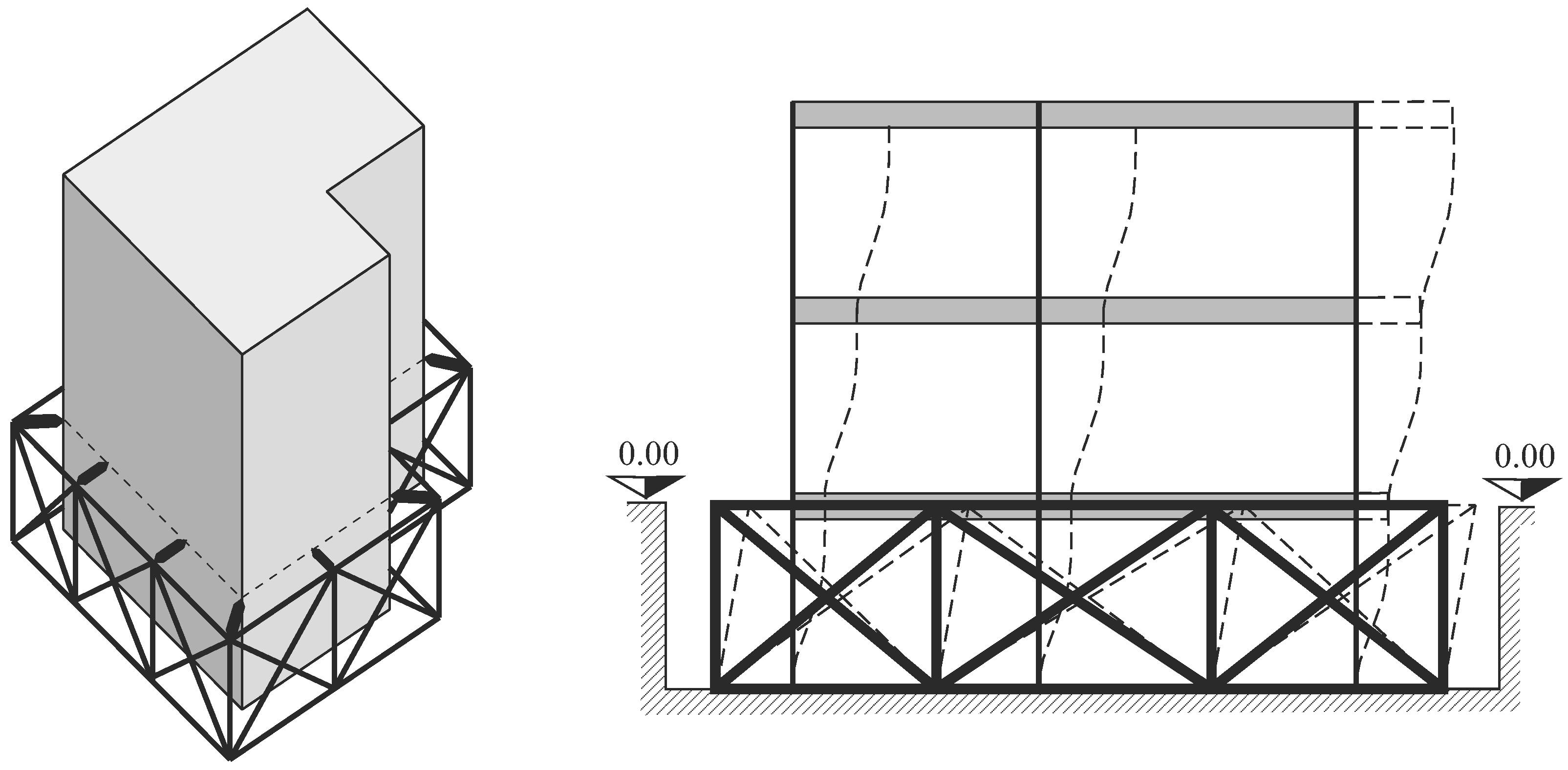
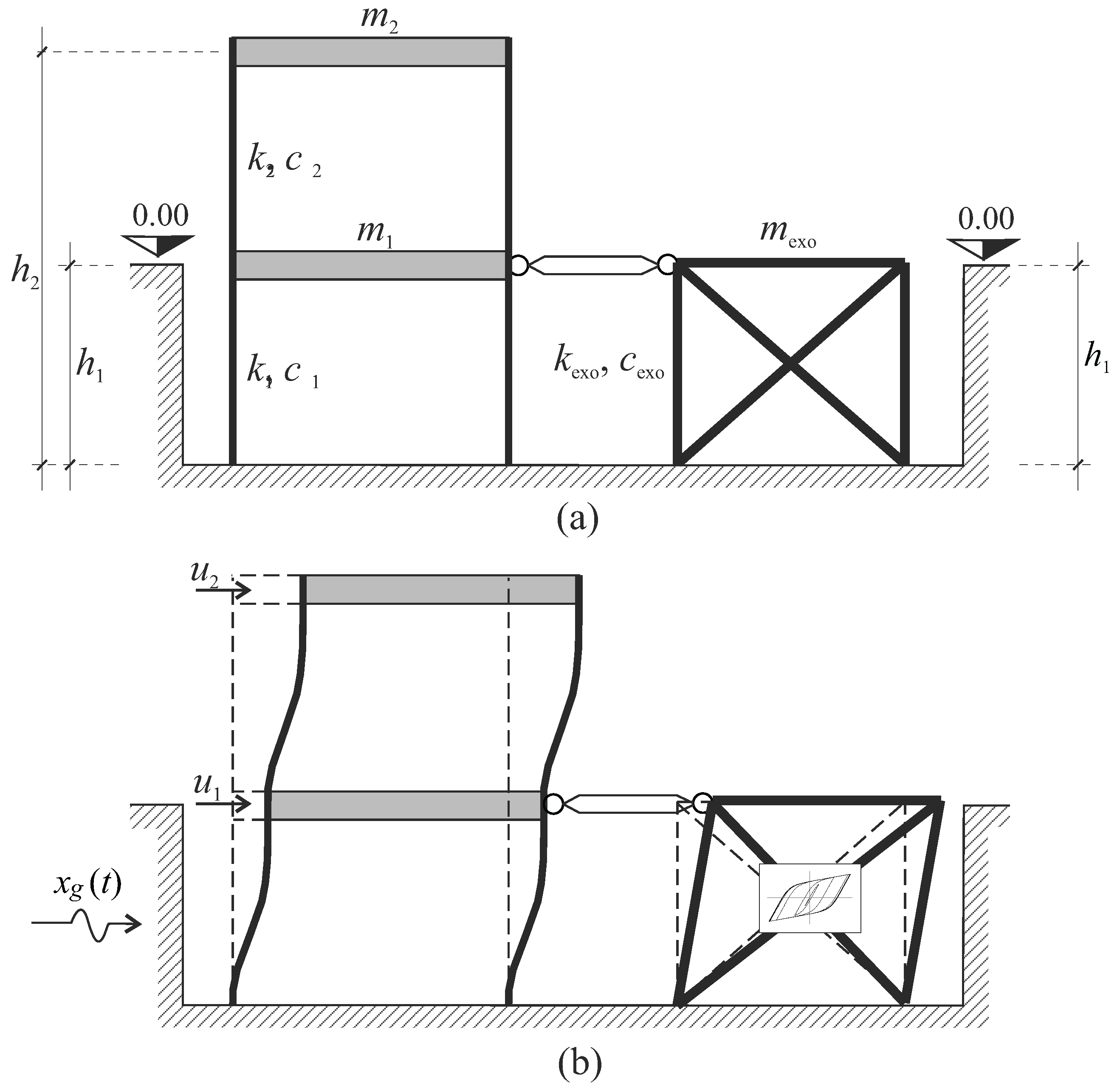
3. Mechanical System

Regardless of the number of storeys, the structure is modelled by an equivalent 2-DOF system (Figure 2a), in which the first DOF, $u_1$, is associated with the sub-structure and the second one, $u_2$, is associated with the super-structure (Figure 2b). The exoskeleton is modelled by a 1-DOF yielding system. Due to the rigid connection between mass $m_1$, which is associated with the displacement $u_1$ of the equivalent 2-DOF system, and the yielding system, the coupled system has the same number of degrees of freedom as the model of the stand-alone structure.

Starting from a given multiple-degree of freedom (M-DOF) sufficiently regular frame structure, the mechanical characteristics of the equivalent 2-DOF system derive from the procedure presented in [36,37,38]. Such a procedure is applied to derive the equivalent stiffnesses, $k_1$ and $k_2$, that are associated to the two DOF. Masses $m_1$ and $m_2$ coincide with the physical masses of the sub-structure and super-structure, respectively. According to the same procedure, the two DOF, $u_1$ and $u_2$, represent the displacements of the floor connected to the yielding system and of the top floor of the structure, respectively. The two damping coefficients of the 2-DOF model, $c_1$ and $c_2$, are derived from the Rayleigh formulation, assuming a damping ratio $\xi =0.05$ for both the oscillation modes of the model.

The mechanical characteristics of the yielding 1-DOF system $m_{\mathrm{exo}}$ and $k_{\mathrm{exo}}$ are the parameters varied in the analyses. In particular, $k_{\mathrm{exo}}$ is the linear elastic stiffness, before the plastic deformation, whereas the damping coefficient $c_{\mathrm{exo}}$ is obtained by treating the stand-alone yielding system as a 1-DOF elastic system. Specifically, $c_{\mathrm{exo}}=2{\xi }_{\mathrm{exo}}{m}_{\mathrm{exo}}{\omega }_{\mathrm{exo}}$, with ${\omega }_{\mathrm{exo}}=\sqrt{k_{\mathrm{exo}}/m_{\mathrm{exo}}}$ (${\xi }_{\mathrm{exo}}=0.02$).

3.1. Equations of Motion

The equations of motion are derived by imposing the equilibrium of the forces acting on $m_1$ and $m_2$,

$$\begin{array}{c}(m_1+m_{\mathrm{exo}}){\ddot{u}}_1\left(t\right)+(c_1+c_2+c_{\mathrm{exo}}){\dot{u}}_1\left(t\right)-c_2{\dot{u}}_2\left(t\right)+\hfill \\ (k_1+k_2)u_1\left(t\right)-k_2{u}_2\left(t\right)+f_{\mathrm{exo}}\left(t\right)=-(m_1+m_{\mathrm{exo}}){\ddot{x}}_g\left(t\right)\hfill \\ m_2{\ddot{u}}_2\left(t\right)-c_2{\dot{u}}_1\left(t\right)+c_2{\dot{u}}_2\left(t\right)-k_2{u}_1\left(t\right)+k_2{u}_2\left(t\right)=-m_2{\ddot{x}}_g\left(t\right)\hfill \end{array}$$

(1)

where ${\ddot{x}}_g$ is the external base excitation, and $f_{\mathrm{exo}}$ is the restoring force describing the constitutive behaviour of the yielding system.

3.2. Elasto-Plastic Description of the Yielding System

The elasto-plastic constitutive behaviour of the yielding system is described by the Bouc-Wen model [22]. According to this model, the restoring force $f_{\mathrm{exo}}$ can be expressed as

$$f_{\mathrm{exo}}\left(t\right)=\psi k_{\mathrm{exo}}{u}_1\left(t\right)+k_{\mathrm{exo}}{u}_y(1-\psi )z_{\mathrm{exo}}\left(t\right)$$

(2)

where $\psi$ is the ratio between the post-yielding stiffness $k_{\mathrm{plast}}$ and the pre-yielding stiffness $k_{\mathrm{exo}}$, i.e., $k_{\mathrm{plast}}=\psi k_{\mathrm{exo}}$. The case $\psi =0$ represents the elastic–perfectly plastic constitutive behaviour of the yielding system, whereas the case $\psi =1$ describes its fully elastic constitutive behaviour. Quantity $u_y$ is the yield displacement, beyond which the yielding system undergoes plastic deformations. It is worth observing that the product $k_{\mathrm{exo}}{u}_y$ represents the yielding force of the structure, $F_y$. Finally, $z_{\mathrm{exo}}$ is an auxiliary variable the describes the post-yielding behaviour and is defined by an ordinary differential equation

$${\dot{z}}_{\mathrm{exo}}\left(t\right)=\frac{1}{u_y}\left[A-{\left|z_{\mathrm{exo}}\left(t\right)\right|}^n\left({\beta }_1+{\gamma }_1\mathrm{sign}({\dot{u}}_1\left(t\right)·z_{\mathrm{exo}}\left(t\right))\right)\right]{\dot{u}}_1\left(t\right)$$

(3)

where parameters A, ${\beta }_1$, and ${\gamma }_1$ depend on the shape of the hysteretic cycles.

The parameters of the Bouc-Wen model are functionally redundant; there are multiple sets of values of the parameters that produce identical responses for a given excitation. This redundancy can be removed by fixing one of the parameters. A possibility is to fix $A=1$ so that the physical meaning of the initial stiffness $k_{\mathrm{exo}}=F_y/u_y$ is restored [39].

Parameters ${\beta }_1$ and ${\gamma }_1$ control the shape and size of the hysteretic loop, as demonstrated in [22]. However, they lack any physical interpretation. As suggested in [40], it is assumed ${\beta }_1+{\gamma }_1=1$. The two constraints ${\beta }_1+{\gamma }_1=1$ and $A=1$ reduce the Bouc-Wen model to a strain-softening formulation with a defined meaning of the mechanical quantities $F_y$, $u_y$, $\psi$. Under such constraints, the dimensionless hysteretic parameter $z_{\mathrm{exo}}$ takes values in the range $[-1,1]$. Finally, the exponential parameter n governs the abruptness of the transition between the elastic and post-elastic branch of the hysteresis model. For large values of n, the response approaches that of a bilinear model. All simulations presented in this paper are performed considering $n=2$.

The equations of motions, Equations (1)–(3), are solved numerically, using the Runge–Kutta method, embedded in the command NDSolve inside the Wolfram Mathematica^® environment. The used integration time-step is 0.001 s.

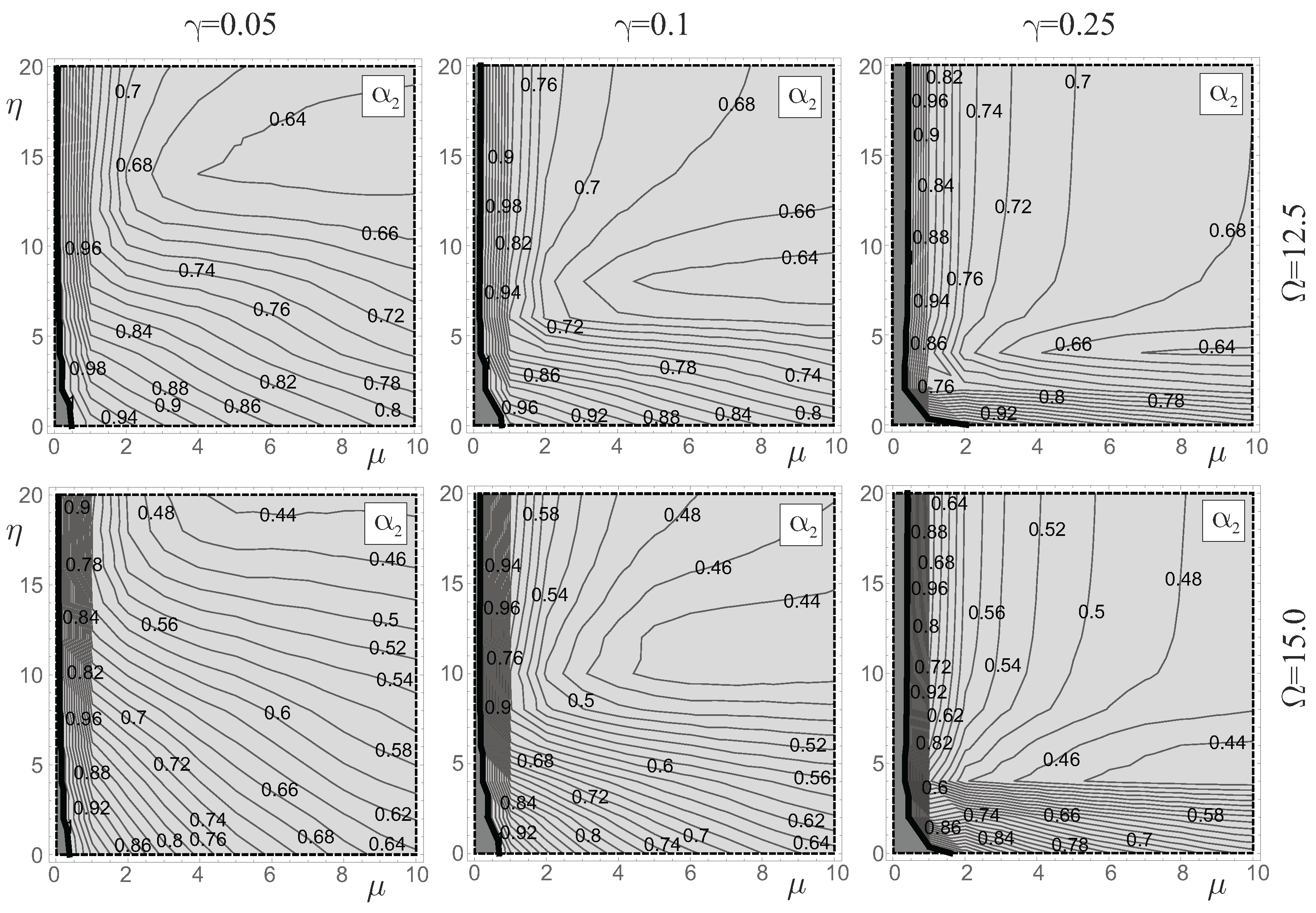
4. Parametric Analysis

Parametric analyses are performed to evaluate the dynamic and the seismic effectiveness of the coupling. To simulate cases close to reality, two structures with characteristics reported in

Table 1. Geometric and mechanical characteristics of the two reference multi-degree-of-freedom frames (M-DOF).

Storeys	Storey Area	Storey Mass ${\mathit{m}}_{\mathbf{s}}$	Storey Height	Main Period
3	100 m${}^2$	$120.6\times {10}^3$ kg	3 m	0.390 s
6	300 m${}^2$	$361.8\times {10}^3$ kg	3 m	0.655 s

are used as references. For each structure, all storeys have the same mass, height, and stiffness. The characteristics reported in Table 1 are used in the reducing order technique adopted in [36,37,38] to derive the mechanical characteristics of equivalent 2-DOF models of the structures.

It is worth observing that the values of $k_1$ and $k_2$ change with the yielding system connection level, even if the equivalent 2-DOF models refer to the same building (see the second and the third rows of

Table 2. Mechanical characteristics of the 2-DOF equivalent systems.

Storeys	Connection	${\mathit{k}}_1$ [N/m]	${\mathit{k}}_2$ [N/m]	${\mathit{m}}_1$ [kg]	${\mathit{m}}_2$ [kg]	$\mathit{\xi }$
3	1	$2.19219\times {10}^8$	$0.93951\times {10}^8$	$120.6\times {10}^3$	$241.2\times {10}^3$	0.05
6	1	$1.02972\times {10}^9$	$1.99300\times {10}^8$	$361.8\times {10}^3$	$1809.0\times {10}^3$	0.05
6	2	$9.30067\times {10}^8$	$1.99300\times {10}^8$	$723.6\times {10}^3$	$1447.2\times {10}^3$	0.05

). In Table 2, $\xi$ shows the modal damping ratio adopted for the two oscillation modes of the stand-alone 2-DOF equivalent model. The value $\xi =0.05$ is commonly used in various building codes for structural frame structures, independently of the material of the structure, and it is the value used in this paper.

The parameters that are varied in the analyses are the following:

• Mechanical characteristics of the 2-DOF system $m_i$ and $k_i$$(i=1,2)$, representing real M-DOF frame structures;
• Post- and pre-yielding stiffness ratio

  $$\psi =\frac{k_{\mathrm{plast}}}{k_{\mathrm{exo}}};$$

  (4)
• Ratio between pre-yielding stiffness of the yielding system and stiffness of the sub-structure

  $$\mu =\frac{k_{\mathrm{exo}}}{k_1};$$

  (5)
• Ratio between yielding force and weight of the yielding system $w_{\mathrm{exo}}$ (obtained multiplying the mass $m_{\mathrm{exo}}$ by the gravitational acceleration g)

  $$\eta =\frac{F_y}{w_{\mathrm{exo}}}=\frac{k_{\mathrm{exo}}{u}_y}{m_{\mathrm{exo}}g};$$

  (6)
• Ratio between mass of the yielding system and total mass of the structure

  $$\gamma =\frac{m_{\mathrm{exo}}}{m_1+m_2}.$$

  (7)

The comparison between the displacement $u_1$ and the drift $\Delta u=u_2-u_1$ of the coupled system and those of the stand-alone structure provides an indication of the efficiency of the coupling. The above-mentioned comparison is performed by means of two gain indexes

$${\alpha }_1=\frac{max\left|u_1\left(t\right)\right|}{max\left|{\tilde{u}}_1\left(t\right)\right|},{\alpha }_2=\frac{max\left|u_2\left(t\right)-u_1\left(t\right)\right|}{max\left|{\tilde{u}}_2\left(t\right)-{\tilde{u}}_1\left(t\right)\right|}=\frac{max\left|\Delta u\left(t\right)\right|}{max\left|\Delta \tilde{u}\left(t\right)\right|}$$

(8)

where the displacements ${\tilde{u}}_1$ and ${\tilde{u}}_2$ are those of the 2-DOF model of the stand-alone structure. According to Equation (8), the effectiveness of the coupling increases as the values of ${\alpha }_1$ and ${\alpha }_2$ become smaller and smaller compared to unity.

The parametric analysis is performed by evaluating the gain indexes ${\alpha }_1$ and ${\alpha }_2$ for each set of variable parameters and a single base motion and plotting such values in a specific parameters plane, thus creating gain maps.

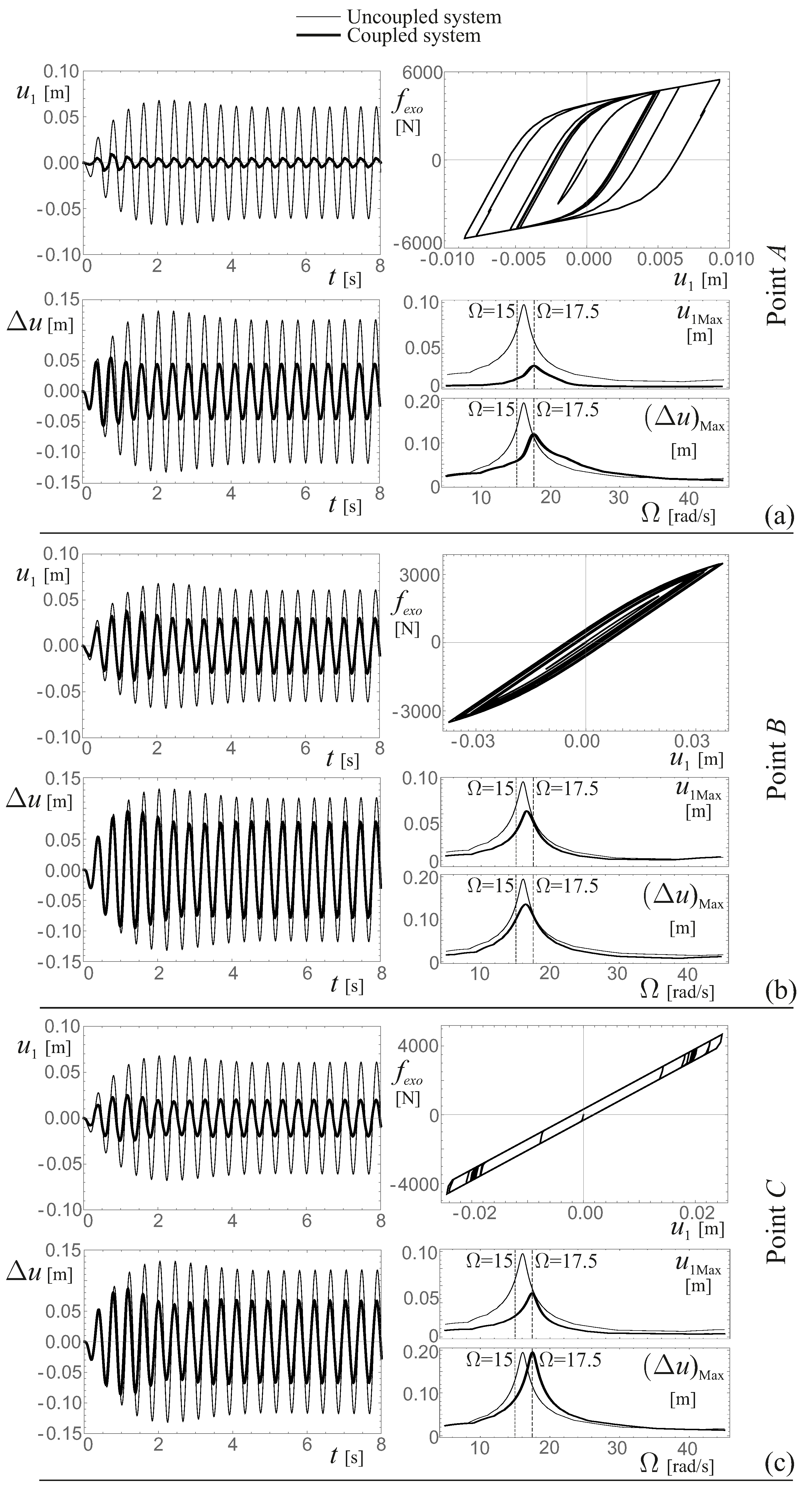
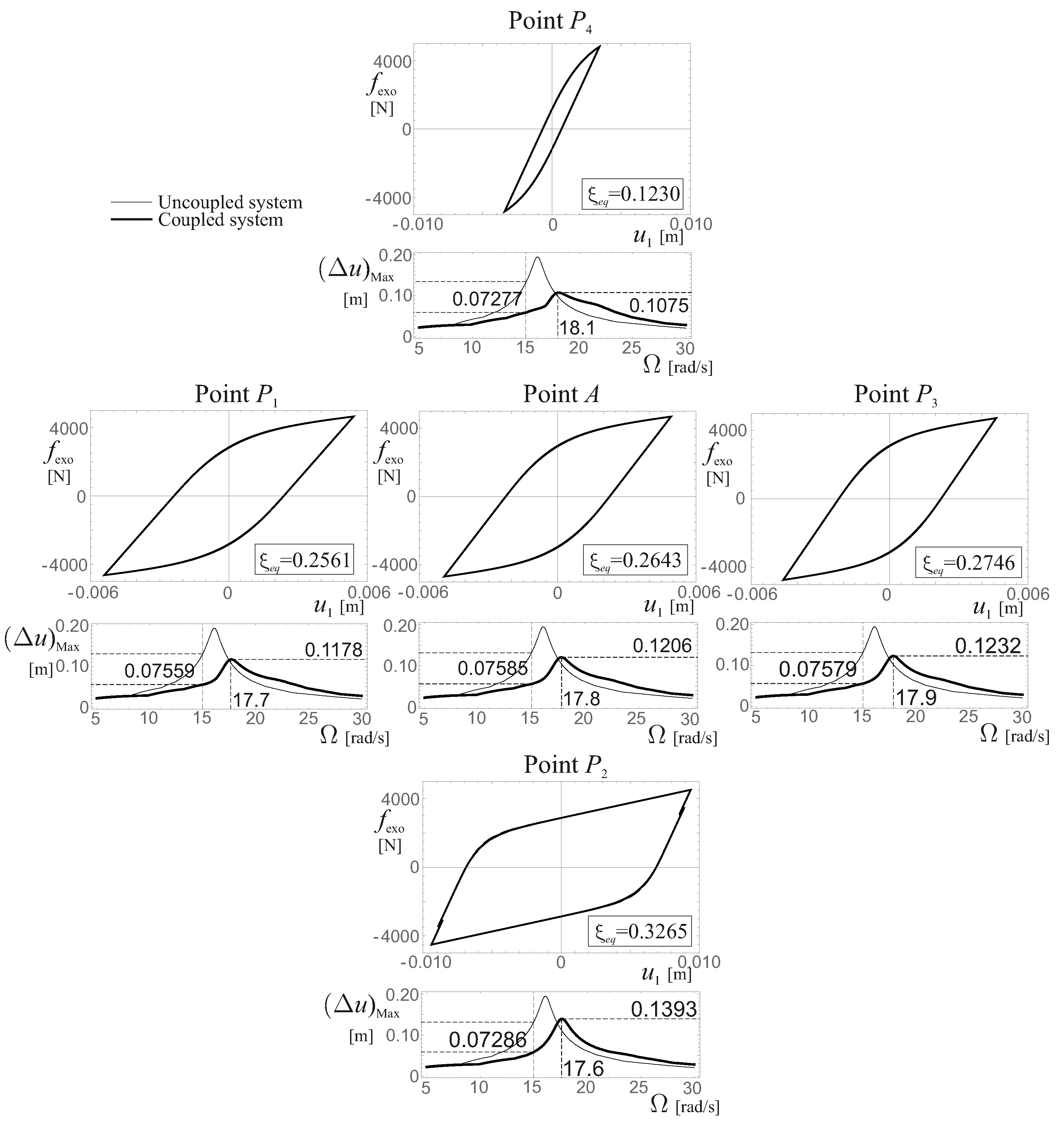
5. Harmonic Excitation

A harmonic excitation

$${\ddot{x}}_g\left(t\right)=A_{s}sin\left(\mathrm{\Omega }t\right)$$

(9)

is used to compare the dynamics of the coupled system and stand-alone structure. In Equation (9), $\mathrm{\Omega }=2\pi /T_s$ is the circular frequency of the excitation, $T_s$ is the period of the harmonic cycle, and $A_s$ is its amplitude.

5.1. The Role of the Elastic Stiffness and of the Yielding Force

The role of $k_{\mathrm{exo}}$ and $F_y$ in the dynamic response of the coupled system is investigated by plotting the gain indexes in the parameters’ plane ($\mu$–$\eta$) (see Equations (5) and (6)). The harmonic analysis is carried out for the three-storey frame structure whose geometric and mechanical characteristics are reported in the first row of Table 1 and Table 2. The main period of the coupled system depends on the mass of the exoskeleton, which is considered fixed ($\gamma =0.1$), and on the stiffness of the exoskeleton, which is accounted for by the parameter $\mu$. Since the gain maps are represented in the parameter plane $\mu$–$\eta$, the range of the main period of the coupled system depends only on $\mu$, which is varied in the range 0–10. Hence, in the parametric analyses performed on the three-storey frame structure, the range of the main periods of the coupled system is approximately 0.32–0.39 s.

As shown in Figure 3a, the yielding system is connected to the first storey of the structure. The gain maps in Figure 3b are contour plots of the gain indexes ${\alpha }_1$ and ${\alpha }_2$ in the parameters’ plane ($\mu$–$\eta$). The light grey colour regions (named advantage regions) are the regions where the gain coefficient is lower than unity, i.e., the coupling with the yielding system reduces the displacements of the structure. In Figure 3b, the two maps of each row refer to the ${\alpha }_1$ (left map) and ${\alpha }_2$ (right map) indexes, which are evaluated for a different $\mathrm{\Omega }$.

The maps in the first column of Figure 3b show that the coupling with the yielding system leads to a significant reduction in $u_1$. In the ${\alpha }_1$ maps, the advantage regions cover almost all the parameters plane, reaching values smaller than 0.1 (i.e., the coupling has the effect to reduce $u_1$ up to $90\%$ of its original value). The ${\alpha }_2$ maps show that the reduction in $\Delta u$ is significantly smaller that the reduction in $u_1$. Although ${\alpha }_2$ has higher values than ${\alpha }_1$, up to $\mathrm{\Omega }=15$ rad/s, the advantage regions still cover almost the entire parameters plane. For frequencies higher than $\mathrm{\Omega }=15$ rad/s, the advantage region shrinks, and the value of ${\alpha }_2$ increases. However, contrarily to ${\alpha }_1$, ${\alpha }_2$ has an absolute minimum inside the investigated parameters’ range. Such minimum depends on $\mathrm{\Omega }$; the smallest value among the minimums (${\alpha }_2=0.42$) is obtained for $\mathrm{\Omega }=15$ rad/s. Such points of minimum provide the optimal design characteristics of the yielding system that lead to the maximum reduction in the drift of the super-structure.

To gain a better understanding of the changes in the dynamics of the coupled system, different mechanical characteristics of the coupling are considered. Specifically, points A, B, and C on the maps referring to $\mathrm{\Omega }=15$ rad/s of Figure 3b are investigated. The results are shown in Figure 4, which is arranged in three sub-figures (a, b, and c). Each sub-figure shows (i) the comparison among time-histories of $u_1\left(t\right)$ and $\Delta u\left(t\right)$ of the coupled system and stand-alone structure (upper ad lower-left graphs), (ii) the hysteretic cycle of the yielding system (upper right graph), and (iii) the comparison of the frequency-response curves of $u_1\left(t\right)$ and $\Delta u\left(t\right)$, referring to the coupled system and stand-alone structure (lower right graph). In the figure, a thick line is used for the coupled system, whereas a thin line is used for the stand-alone structure.

Figure 4a shows the behaviour of the system having mechanical characteristics given by point A, which is the point that corresponds to the absolute minimum of ${\alpha }_2$ in the map obtained for $\mathrm{\Omega }=15$ rad/s. The comparisons between the time-histories of the coupled system and those of the stand-alone structure reveal that the yielding system reduces both $u_1$ and $\Delta u$. The hysteretic cycle shows a significant energy dissipation due to the plastic deformation of the yielding system. The observation of the frequency-response curves reveals a slight increase in the main frequency of the coupled system with respect to the stand-alone structure and a reduction in the amplitude of the displacements, mostly for $u_1$. The two vertical dashed lines reported in all the frequency-response curves correspond to $\mathrm{\Omega }=15$ and $\mathrm{\Omega }=17.5$ rad/s. Along the line that refers to $\mathrm{\Omega }=15$, both $u_1$ and $\Delta u$ of the coupled system have maximum amplitudes smaller than those of the stand-alone structure, since the frequency-response curves of the coupled system are below the curves of the stand-alone structure. In fact, point A is inside the advantage regions of both maps obtained for $\mathrm{\Omega }=15$ rad/s. On the contrary, along the vertical line passing through $\mathrm{\Omega }=17.5$ rad/s, the drift of the coupled system has a maximum value slightly higher than that of the stand-alone structure, and point A is outside the advantage region of the ${\alpha }_2$ map obtained for $\mathrm{\Omega }=17.5$ rad/s (see Figure 3b).

Figure 4b shows the behaviour of the system having mechanical characteristics represented by point B. In this case, such a point is inside the advantage regions of both the ${\alpha }_1$ and ${\alpha }_2$ maps, although it is close to the boundaries of these regions, and the values of the gain indexes approach the unity. In this case, the difference between the maximum amplitudes of the coupled system and stand-alone structure is smaller than the corresponding difference for the structures identified by point A. Instead, the hysteretic cycle shows a small energy dissipation, because the yielding system has very small plastic deformations. Compared to the case described by point A, the frequency-response curves show a smaller reduction in the amplitudes of $u_1$ and $\Delta u$ due to the coupling. Along the lines that refer to $\mathrm{\Omega }=15$ and $\mathrm{\Omega }=17.5$ rad/s, both $u_1$ and $\Delta u$ of the coupled system have maximum amplitudes slightly smaller than those of the stand-alone structure. In fact, point B is inside the advantage regions in both maps obtained for $\mathrm{\Omega }=15$ and $\mathrm{\Omega }=17.5$ rad/s (see Figure 3b).

Figure 4c shows the behaviour of the coupled system with mechanical characteristics represented by point C. Such a point is inside the advantage regions of both the ${\alpha }_1$ and ${\alpha }_2$ maps. The comparisons among time-histories show results coherent with the values of ${\alpha }_1$ and ${\alpha }_2$ at point C. By referring to the hysteretic cycle, due to the small value of the parameter $\eta$ at point C (i.e., small value of the yield displacement $u_y$), there are large plastic deformations of the yielding system that, nevertheless, provide limited energy dissipation. The frequency-response curves show that the coupling does not affect the maximum amplitude of $\Delta u$ but provides only a shift towards higher values of the main frequency of the coupled system. Along the lines for $\mathrm{\Omega }=15$ rad/s, both $u_1$ and $\Delta u$ of the coupled system have maximum amplitudes smaller than those of the stand-alone structure and, coherently, point C is inside the advantage regions of both maps obtained for $\mathrm{\Omega }=15$. On the contrary, along the lines for $\mathrm{\Omega }=17.5$ rad/s, only $u_1$ slightly decreases after the coupling. Instead, the $\Delta u$ of the coupled system is significantly higher than the one of the stand-alone structure. This occurrence is coherent with point C being inside the advantage region of the ${\alpha }_1$ map and outside the advantage region of the ${\alpha }_2$ map obtained for $\mathrm{\Omega }=17.5$ rad/s (see Figure 3b). Additionally, an almost resonance condition occurs at point C for the coupled system, since the main frequencies of the system and harmonic excitation are close to each other.

During the harmonic excitation, after the transient dynamics, the coupled system reaches a dynamic motion characterised by stationary hysteretic cycles. To further explain the effects of the coupling, the equivalent damping ratio ${\xi }_{eq}$ of such stationary hysteretic cycles is evaluated. The value of ${\xi }_{eq}$ is obtained by equating the area of the hysteretic cycle $E_h$ and the area of the cycle $E_v$ of an equivalent linear viscous damped system under the same excitation. As in [41], the area of the equivalent viscous cycle is evaluated as $E_v=\pi c_{eq}{\omega }_{eq}{\tilde{u}}_1$, where $c_{eq}$ and ${\omega }_{eq}$ are the damping coefficient and the frequency of the equivalent viscous system, respectively, and ${\tilde{u}}_1$ is the maximum displacement of the hysteretic system that corresponds to the maximum strain of the equivalent system. For a linear viscous 1-DOF system $c_{eq}=2{\xi }_{eq}{\omega }_{eq}m$, ${\omega }_{eq}=\sqrt{k_{eq}/m}$, and $k_{eq}$ can be related to the maximum restoring force reached in the hysteretic cycle ${\tilde{f}}_{\mathrm{exo}}$ and to ${\tilde{u}}_1$ ($k_{eq}={\tilde{f}}_{\mathrm{exo}}/{\tilde{u}}_1$); thus, the equivalent damping ratio reads

$${\xi }_{eq}=\frac{E_h}{2\pi {\tilde{u}}_1{\tilde{f}}_{\mathrm{exo}}}$$

(10)

Figure 5 shows the stationary hysteretic cycles and the frequency-response curves of $\Delta u$ that are related to points A and $P_i(i=1,\dots ,4)$. Such points are shown in the ${\alpha }_2$ map obtained for $\mathrm{\Omega }=15$ rad/s of Figure 3b. Specifically, A is located at the point of absolute minimum, whereas the other points $P_i$ are in the vicinity of A. For each investigated point, ${\xi }_{eq}$ is reported near the plot of the limit cycle. For each plot, the frequency-response curves of the drift show (i) the main frequency of the coupled system and the maximum value of drift (thick curve), and (ii) the difference between the maximum drift of the coupled system and stand-alone structure at $\mathrm{\Omega }=15$ rad/s (the same frequency of the map on which points A and $P_i$ are located). Along the horizontal direction (from point $P_1$ to $P_3$, passing through A), although numerically close to each other, the values of ${\xi }_{eq}$ slightly increase. Moreover, the increase in the pre-yielding stiffness of the yielding system, measured by the parameter $\mu$, causes an increase in the main frequency of the coupled system and a minor increase in its maximum drift. These different effects combine in such a way that the largest difference between the drifts of the coupled system and stand-alone system along $\mathrm{\Omega }=15$ rad/s occurs at point A.

Along the vertical direction (from point $P_2$ to $P_4$, passing through A), the increase of the yielding displacement, which is measured by the parameter $\eta$, causes a decrease in the equivalent damping of the hysteretic cycles. Additionally, the main frequency of the coupled system increases, and the maximum drift in correspondence of the main frequency decreases. Along the vertical direction, the different effects combine so that the coupling is more effective for the characteristics of the coupled system defined by point A. Figure 5 also shows that the frequency-response curves have significantly different shapes of the descending branches (i.e., the branch on the right of the main frequency).

5.2. The Role of the Post-Elastic Stiffness and of the Mass of the Yielding System

This subsection analyses the sensitivity of the dynamics of the coupled system to $\psi$. Since the coupling with the yielding system is always beneficial for the sub-structure, Figure 6 shows only the ${\alpha }_2$ maps that are related to the super-structure. The maps are arranged in matrix form, where the rows refer to different $\mathrm{\Omega }$ and the columns refer to different values of $\psi$. For both values of $\mathrm{\Omega }$, the increase in $\psi$ results in a decrease in the effectiveness of the coupling. As general effect of the increase in $\psi$, the contour levels of the maps tend to become vertical, and the point of absolute minimum of the drift disappears from the investigated range of the parameters. When $\psi =1$, the yielding system has a linear elastic behaviour, and the response of the coupled system does not depend on $u_y$ or equivalently on $\eta$.

A second analysis shows the dependence of the dynamics of the coupled system on the mass of the yielding system, which is parametrically measured by $\gamma$. In addition, in this case, Figure 7 only shows the ${\alpha }_2$ maps referring to the super-structure. Such maps are arranged in matrix form, where the rows refer to different $\mathrm{\Omega }$ and the columns refer to different values of $\gamma$. For both values of $\mathrm{\Omega }$, the increase in $\gamma$ significantly changes the maps. Nevertheless, the effectiveness of the coupling is not affected by $\gamma$, since the minimum values reached by ${\alpha }_2$ when $\gamma$ changes remain the same. The increase in $\gamma$ mainly affects the vertical position of the absolute minimum of ${\alpha }_2$. Specifically, as $\gamma$ increases, the value of $\eta$ that corresponds to the minimum value of ${\alpha }_2$ decreases. Finally, it is worth observing that the value of $\mu$ where the minimum of ${\alpha }_2$ occurs does not significantly depend on $\gamma$.

5.3. The Role of the Amplitude of the Harmonic Excitation

The coupled system is described by nonlinear equations due to the hysteretic constitutive behaviour of the yielding system. Consequently, the response of the coupled system depends on $A_s$. This subsection analyses the sensitivity of the dynamics of the coupled system to $A_s$. Figure 8a shows the ${\alpha }_2$ gain maps, referring to the harmonic frequency $\mathrm{\Omega }=12.5$ rad/s, and obtained for different values of $A_s$ (from left to right, $A_s$ varies from 0.5 to 1.0 g). The effectiveness of the coupling is not affected by $A_s$, since the minimum values reached by ${\alpha }_2$ are the same in all of the maps. When $A_s$ increases, the value of $\eta$ at which the minimum value of ${\alpha }_2$ occurs increases as well. It is worth observing that the value of $\mu$ for which the minimum of ${\alpha }_2$ occurs does not depend on $A_s$. Figure 8b shows the stationary hysteretic cycles corresponding to the minimum points A indicated in Figure 8a. It is interesting to note that although the areas of these cycles are very different to each other, ${\xi }_{eq}$ remains almost constant (${\xi }_{eq} \cong$ 0.301).

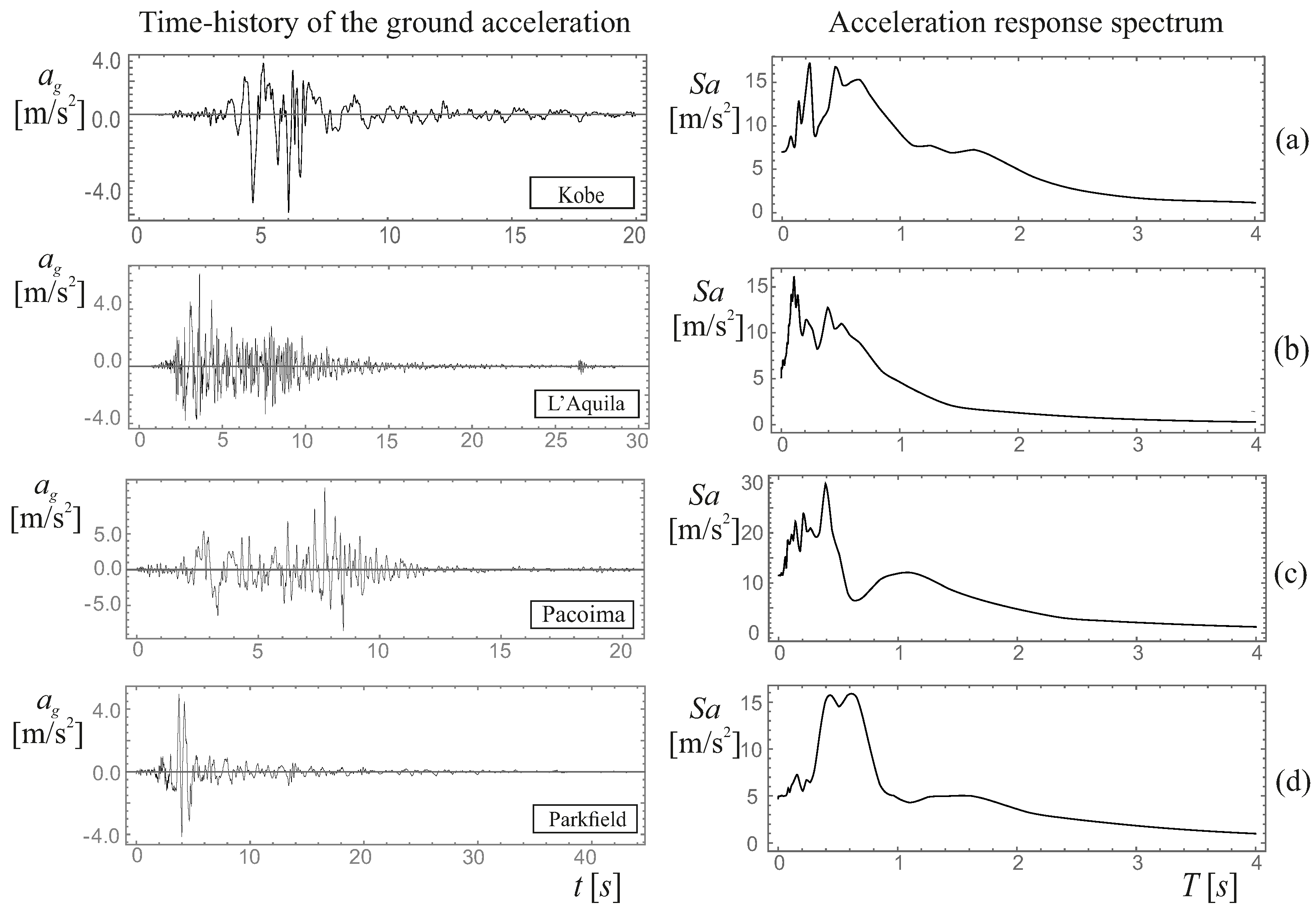
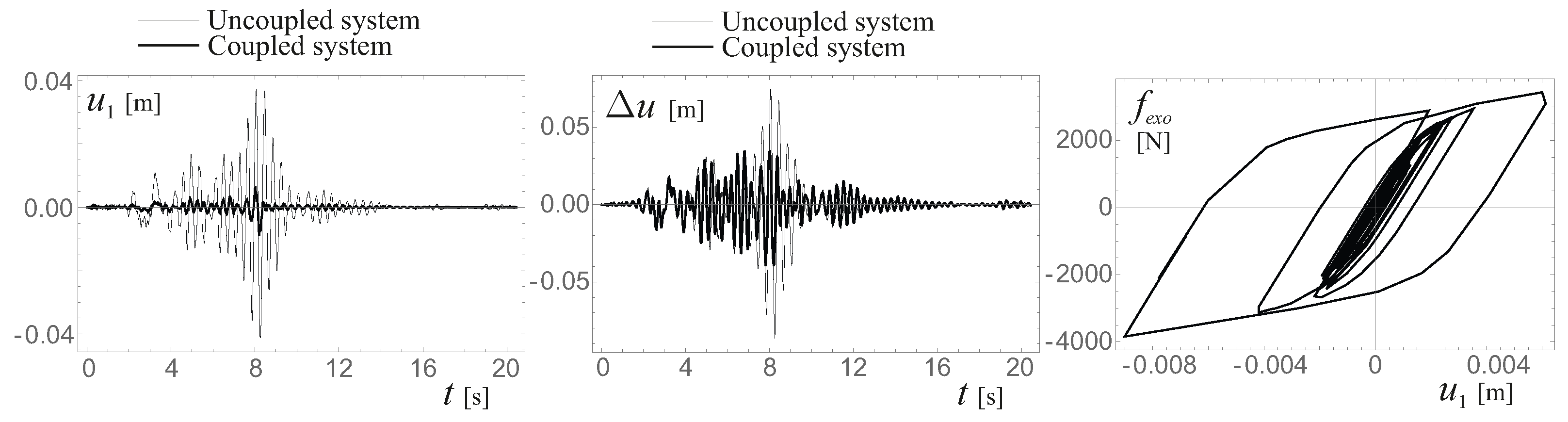
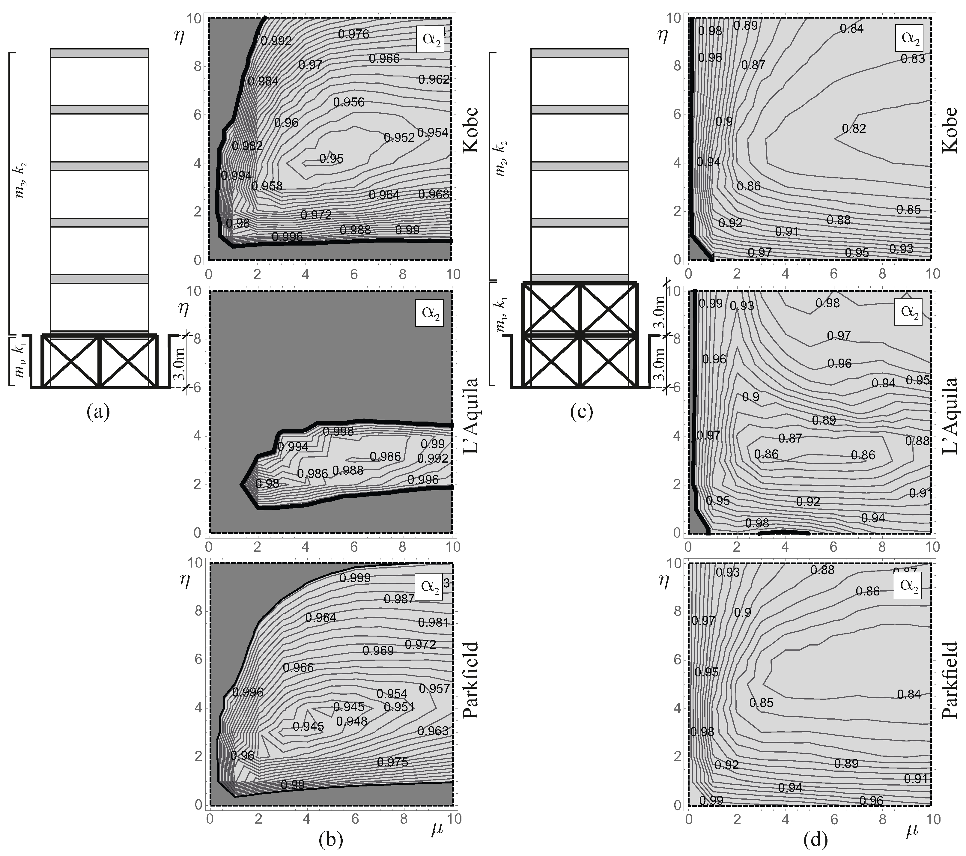
6. Seismic Excitation

A set of four earthquake records is used as excitation for the seismic analyses. The selection of the records is performed accounting for the differences in the spectral characteristics of the earthquake records. The limited number of earthquake records does not directly allow assessing the sensitivity of the results on the features of the records but provides a significant indication about the ability of the exoskeleton to improve the seismic performance of frame structures. Figure 9 shows the time-histories of the selected records in the left column and the corresponding pseudo-acceleration elastic spectra on the right column. The considered earthquake records are

(a)

Kobe, Takarazuka-000 station, ground motion recorded during the 1995 Japan earthquake;

(b)

L’Aquila, IT.AQV.HNE.D.20090406.013240.X.ACC station, ground motion recorded during the 2009 Italian earthquake;

(c)

Pacoima, Dam-164 ground motion recorded during the 1971 San Fernando, California earthquake;

(d)

Parkfield, CO2-065 ground motion recorded during the California earthquake 1966.

In the following, each record is called with the underlined name of the above list. In this case, the results are obtained by numerically integrating the equations of motion (Equation (1)).

Discussion of the Results

The first seismic analysis considers the structure whose geometric and mechanical characteristics are reported in the first rows of Table 1 and Table 2, i.e., the three-storey frame structure. For this structure, the range of the main periods of the coupled system is approximately 0.32–0.39 s, as for the analysis with harmonic excitation. As shown in Figure 10a, the coupling with the yielding system is performed at the first storey of the structure. Both the ${\alpha }_1$ and ${\alpha }_2$ gain maps are reported in Figure 10b. When the coupled system is excited by the four records, the coupling reduces the displacements of the sub-structure. The gain index ${\alpha }_1$ reaches values of about 0.1, which means a reduction of $u_1$ of about 90% with respect to the stand-alone structure. As occurs for the harmonic excitation, also under seismic excitation, the ${\alpha }_2$ maps present points with absolute minima. The position of these points and the corresponding values of ${\alpha }_2$ vary with the records. Nevertheless, for all records, there is a reduction in the drift of the coupled system. For example, for the Kobe earthquake, for which the coupling is less effective, the minimum value of ${\alpha }_2$ is about 0.66, which entails about a 30% reduction of the drift compared to the stand-alone structure.

Figure 11 shows the time-histories of $u_1\left(t\right)$ and $\Delta u\left(t\right)$ together with the hysteretic cycle. Such curves refer to the point labelled with A in the Pacoima maps of Figure 10. The comparison between the time-histories of the coupled system (thick line) and those of the stand-alone structure (thin line) shows a notable reduction in both the displacement of the sub-structure and the drift of the super-structure due to the coupling. Moreover, the hysteretic cycle in Figure 11 clearly shows the yielding of the system and the consequent energy dissipation.

The last seismic analysis considers a structure whose geometric and mechanical characteristics are reported in the second row of Table 1 (six-storey building). Figure 12 shows only the ${\alpha }_2$ maps because also in this case, the coupling is always beneficial for the sub-structure. The results refer to three different earthquakes records (Kobe, L’Aquila, and Parkfield). In this analysis, the connection between the structure and the yielding system is placed at either the first or second storey. In this case, the main period of the coupled system varies in the range 0.60–0.66s when the connection with the exoskeleton is at the first storey of the frame structure and in the range 0.61–0.66 s when the connection is at the second storey. The mechanical characteristics of the 2-DOF system that represent the coupled system are reported in the second and third row of Table 2.

Figure 12a shows the scheme of the connection. The ${\alpha }_2$ maps of this structural scheme are shown in Figure 12b. The advantage regions cover a limited portion of the parameters plane and reach minimum values close to unity. This means that the reduction of the drift of the super-structure is negligible. The dimension of the yielding system (one storey) is too small with respect to that of the super-structure (five storeys) to be able to change the response of the super-structure. Therefore, a change in the structural scheme is needed. Figure 12c shows a scheme where the connection between the structure and the yielding system is at the second storey. The ${\alpha }_2$ maps referring to this coupled system are shown in Figure 12d. The increase in the dimension of the yielding system (two storeys) and the consequent decrease in the dimension of the super-structure (four storey) with respect to the case in Figure 12a causes the enlargement of the advantage regions. Moreover, the minimum value of ${\alpha }_2$ reduces.

7. Conclusions

In this paper, a 2-DOF model, representing a general N-DOF frame structure, was coupled with an external yielding 1-DOF system, representing an exoskeleton, to improve the dynamic and seismic behaviour of the 2-DOF model. A rigid link connects the bottom mass of the 2-DOF model to the 1-DOF yielding system. Such a yielding system was assumed to have an elasto-plastic constitutive behaviour that was modelled by the Bouc-Wen model. Due to the rigid link between the 2-DOF model of the structure and yielding system, the coupled system was still described by a 2-DOF mechanical model. The nonlinear equations of motion were obtained by a direct approach and successively numerically integrated to analyse the dynamics of the coupled system. The coupling with the yielding system was considered beneficial for the structure in the occurrence of a reduction in the displacements and drifts of the structure.

An extensive parametric analysis was performed, considering both harmonic and seismic excitations. The parameters varied in the analysis were those characterising the elasto-plastic constitutive behaviours of the yielding system. The results were summarised in behaviour maps that provided the ratios between the maximum displacements (or the drift) of the coupled system and the stand-alone structure. In these maps, a ratio less than unity shows that the yielding system is effective in improving the dynamics of the structure.

The analysis showed wide regions of the parameter plane where the coupling is beneficial for the structure. In correspondence of the points of the maps where the best performances occur, the yielding system exhibits a behaviour with hysteretic cycles that have a high value of equivalent damping coefficient. As expected, the performance of the coupled system also depends on its characteristics and on the spectral content of the excitation. Since, in all cases, the coupling with the yielding system is beneficial for the sub-structure, the coupling may be particularly effective in structures with the so-called soft storey, which is usually located at the lower levels of structures. The coupling can reduce the displacement of such storeys up to 90% of their initial values and, at the same time, could improve the dynamic and seismic performances of the super-structure. The results encourage checking the effectiveness of such a method for real structures by using more accurate FEM models. However, the results reveal that if the frame structure to be protected is sufficiently regular, the used low-dimensional models can properly capture the dynamic and seismic behaviour of the structure.

Finally, the main novelties and advantages of the study are summarised below:

• Differently to the use of braced and/or knee-braced frames that are usually distributed in the whole structure, the proposed method uses an exoskeleton that involves only a small part of the structure to be protected.
• Since the connection between the structure and the exoskeleton is performed by rigid links at the level of the first (or second) storey, the mechanical and geometric characteristics of the structure to be protected remain unchanged.
• Although the exoskeleton is shorter than the frame structure, it has the ability to improve the dynamic and seismic response of both the part below the connection with the exoskeleton and the part above such a connection.
• The stiffness and the mass of the exoskeleton are parameters that can be varied easily and that can be used to improve the performances of the coupled system. This possibility is harder to exploit in braced and/or knee-braced frames.

On the contrary, the proposed method has the following limitations:

• The exoskeleton requires some space around the frame structure to protect and could have an undesired aesthetic impact.
• The limited height of the exoskeleton may undermine the effectiveness of the proposed protection for high-rise buildings. For significantly taller frame structures, there may be the need to connect the two structures at higher storeys in order to achieve a significant reduction of the displacements of the superstructure.

References

1. Bachmann, J.; Vassiliou, M.; Stojadinović, B. Dynamics of Rocking Podium Structures. Earthq. Eng. Struct. Dyn. 2017, 46, 2499–2517. [Google Scholar] [CrossRef]
2. Makris, N. A half-century of rocking isolation. Earthq. Struct. 2014, 7, 1187–1221. [Google Scholar] [CrossRef]
3. Aghagholizadeh, M.; Makris, N. Earthquake response analysis of yielding structures coupled with vertically restrained rocking walls. Earthq. Eng. Struct. Dyn. 2018, 47, 2965–2984. [Google Scholar] [CrossRef]
4. Makris, N.; Aghagholizadeh, M. The dynamics of an elastic structure coupled with a rocking wall. Earthq. Eng. Struct. Dyn. 2017, 46, 945–954. [Google Scholar] [CrossRef]
5. Di Egidio, A.; Pagliaro, S.; Fabrizio, C.; de Leo, A. Dynamic response of a linear two d.o.f system visco-elastically coupled with a rigid block. Coupled Syst. Mech. 2019, 8, 351–375. [Google Scholar]
6. Di Egidio, A.; Pagliaro, S.; Fabrizio, C.; de Leo, A. Seismic performance of frame structures coupled with an external rocking wall. Eng. Struct. 2020, 224, 111207. [Google Scholar] [CrossRef]
7. Di Egidio, A.; Pagliaro, S.; Fabrizio, C. Combined use of rocking wall and inerters to improve the seismic response of frame structures. J. Eng. Mech. 2021, 147, 04021016. [Google Scholar] [CrossRef]
8. Pagliaro, S.; Aloisio, A.; Di Egidio, A.; Alaggio, R. Rigid block coupled with a 2 d.o.f. system: Numerical and experimental investigation. Coupled Syst. Mech. 2020, 6, 539–562. [Google Scholar]
9. Impollonia, N.; Palmeri, A. Seismic performance of buildings retrofitted with nonlinear viscous dampers and adjacent reaction towers. Earthq. Eng. Struct. Dyn. 2018, 47, 1329–1351. [Google Scholar] [CrossRef]
10. Zulli, D.; Di Egidio, A. Galloping of internally resonant towers subjected to turbulent wind. Contin. Mech. Thermodyn. 2014, 27, 835–849. [Google Scholar] [CrossRef]
11. Di Egidio, A.; Zulli, D. Critical and post-critical galloping behavior of base isolated coupled towers. Int. J.-Non-Linear Mech. 2021, 134, 103728. [Google Scholar] [CrossRef]
12. Tubaldi, E. Dynamic behavior of adjacent buildings connected by linear viscous/viscoelastic dampers. Struct. Control Health Monit. 2015, 22, 1086–1102. [Google Scholar] [CrossRef]
13. Kelly, J. Base isolation: Linear theory and design. Earthq. Spectra 1995, 6, 223–244. [Google Scholar] [CrossRef]
14. Den Hartog, J.P. Mechanical Vibrations, 4th ed.; McGraw-Hill: New York, NY, USA, 1956. [Google Scholar]
15. Rana, R.; Soong, T. Parametric analysis and simplified design of tuned mass damper. Eng. Struct. 1998, 20, 193–204. [Google Scholar] [CrossRef]
16. Miranda, J.C. On tuned mass dampers for reducing the seismic response of structures. Earthq. Eng. Struct. Dyn. 2005, 34, 847–865. [Google Scholar] [CrossRef]
17. Tsai, H.H. The effect of tuned-mass dampers on the seismic response of base-isolated structures. Int. J. Solid Struct. 1995, 32, 1195–1210. [Google Scholar] [CrossRef]
18. Taniguchi, T.; Kiureghian, A.D.; Melkumyan, M. Effect of tuned mass damper on displacement demand of base-isolated structures. Eng. Struct. 2008, 30, 3478–3488. [Google Scholar] [CrossRef]
19. De Domenico, D.; Ricciardi, G. An enhanced base isolation system equipped with optimal Tuned Mass Damper Inerter (TMDI). Earthq. Eng. Struct. Dyn. 2018, 47, 1169–1192. [Google Scholar] [CrossRef]
20. De Domenico, D.; Impollonia, N.; Ricciardi, G. Soil-dependent optimum design of a new passive vibration control system combining seismic base isolation with tuned inerter damper. Soil Dyn. Earthq. Eng. 2018, 105, 37–53. [Google Scholar] [CrossRef]
21. Giaralis, A.; Taflanidis, A. Optimal tuned mass-damper-inerter (TMDI) design for seismically excited MDOF structures with model uncertainties based on reliability criteria. Struct. Control Health Monit. 2018, 25, e2082. [Google Scholar] [CrossRef]
22. Wen, Y.K. Method for random vibration of hysteretic systems. J. Eng. Mech. 1976, 102, 249–263. [Google Scholar] [CrossRef]
23. Yaghmaei-Sabegh, S.; Safari, S.; Ghayouri, K.A. Estimation of inelastic displacement ratio for base-isolated structures. Earthq. Eng. Struct. Dyn. 2018, 47, 634–659. [Google Scholar] [CrossRef]
24. Scudieri, G. Adaptive building exoskeletons, a biomimetic model for the rehabilitation of social housing. Int. J. Archit. Res. 2015, 9, 134–143. [Google Scholar] [CrossRef] [Green Version]
25. Boake, T. Diagrid Structures: Systems-Connections-Details; Birkhauser: Basel, Switzerland, 2014. [Google Scholar] [CrossRef]
26. Zhu, H.; Ge, D.; Huang, X. Optimum connecting dampers to reduce the seismic responses of parallel structures. J. Sound Vib. 2011, 330, 1931–1949. [Google Scholar] [CrossRef]
27. Reggio, A.; Restuccia, L.; Ferro, G. Feasibility and effectiveness of exoskeleton structures for seismic protection. Procedia Struct. Integr. 2018, 9, 303–310. [Google Scholar] [CrossRef]
28. Thambirajah, B.; Ming-Tuck, S.; Chih-Young, L. Diagonal brace with ductile knee anchor for aseismic steel frame. Earthq. Eng. Struct. Dyn. 1990, 19, 847–858. [Google Scholar]
29. Giuliano, M.; Longo, A.; Montuori, R.; Piluso, V. Influence of homoschedasticity hypothesis of structural response parameters on seismic reliability of CB-frames. Georisk Assess. Manag. Risk Eng. Syst. Geohazards 2011, 5, 120–131. [Google Scholar] [CrossRef]
30. Kari, A.; Ghassemieh, M.; Abolmaali, S. A new dual bracing system for improving the seismic behavior of steel structures. Smart Mater. Struct. 2011, 20, 125020. [Google Scholar] [CrossRef]
31. Kanyilmaz, A. Secondary frame action in concentrically braced frames designed for moderate seismicity: A full scale experimental study. Bull. Earthq. Eng. 2017, 15, 2101–2127. [Google Scholar] [CrossRef]
32. Aninthaneni, P.; Dhakal, R. Prediction of lateral stiffness and fundamental period of concentrically braced frame buildings. Bull. Earthq. Eng. 2017, 15, 3053–3082. [Google Scholar] [CrossRef]
33. Kheyroddin, A.; Mashhadiali, N. Response modification factor of concentrically braced frames with hexagonal pattern of braces. J. Constr. Steel Res. 2018, 148, 658–668. [Google Scholar] [CrossRef]
34. Tian, L.; Qiu, C. Modal pushover analysis of self-centering concentrically braced frames. Struct. Eng. Mech. 2018, 65, 254–261. [Google Scholar]
35. Beiraghi, H. Seismic response of dual structures comprised by Buckling-Restrained Braces (BRB) and RC walls. Struct. Eng. Mech. 2019, 72, 443–454. [Google Scholar]
36. Fabrizio, C.; Di Egidio, A.; de Leo, A. Top disconnection versus base disconnection in structures subjected to harmonic base excitation. Eng. Struct. 2017, 152, 660–670. [Google Scholar] [CrossRef]
37. Fabrizio, C.; de Leo, A.; Di Egidio, A. Tuned mass damper and base isolation: A unitary approach for the seismic protection of conventional frame structures. J. Eng. Mech. 2019, 145, 04019011. [Google Scholar] [CrossRef]
38. Fabrizio, C.; de Leo, A.; Di Egidio, A. Structural disconnection as a general technique to improve the dynamic and seismic response of structures: A basic model. Procedia Eng. 2017, 199, 1635–1640. [Google Scholar] [CrossRef]
39. Ma, F.; Zhang, H.; Bockstedte, A.; Foliente, G.; Paevere, P. Parameter Analysis of the Differential Model of Hysteresis. J. Eng. Mech. 2004, 71, 342–349. [Google Scholar] [CrossRef]
40. Constantinou, M.; Adnane, M. Dynamics of Soil-Base-Isolated Structure Systems: Evaluation of Two Models for Yielding Systems; Report to NSAF; Department of Civil Engineering, Drexel University: Philadelphia, PA, USA, 1987. [Google Scholar]
41. Cheng, F.Y. Matrix Analysis of Structural Dynamics—Applications and Earthquake Engineering; Marcel Dekker, Inc.: New York, NY, USA, 2000; ISBN 0-8427-0387-1. [Google Scholar]
Figure 1. Indicative scheme of the connection between frame structure and exoskeleton.
Applsci 12 10398 g001
Figure 2. Mechanical system: (a) geometric and mechanical characteristics of the system; (b) deformed configuration and positive directions of the Lagrangian parameters.
Applsci 12 10398 g002
Figure 3. Gain maps: (a) geometric coupling scheme; (b) Gain maps α 1 and α 2 for different frequencies Ω of the harmonic excitation ( ψ = 0.1 , γ = 0.1 , A s = 0.7 g m/s 2 ); Points AD and P 1 P 4 denote reference cases examined in the analyses.
Applsci 12 10398 g003
Figure 4. Time-histories, hysteretic cycles and frequency-amplitude curves: (a) Point A; (b) Point B; (c) Point C (points labelled in Figure 3b, ψ = 0.1 , γ = 0.1 , A s = 0.7 g m/s 2 ).
Applsci 12 10398 g004
Figure 5. Stationary hysteretic cycles and frequency-amplitude curves of the drift (points labelled in Figure 3b, ψ = 0.1 , γ = 0.1 , A s = 0.7 g m/s 2 ).
Applsci 12 10398 g005
Figure 6. Gain α 2 maps for different post-elastic stiffness ratios ψ and different frequencies Ω of the harmonic excitation ( γ = 0.1 , A s = 0.7 g m/s 2 ).
Applsci 12 10398 g006
Figure 7. Gain α 2 maps for different mass ratios γ of the yielding system and different frequencies Ω of the harmonic excitation ( ψ = 0.1 , A s = 0.7 g m/s 2 ).
Applsci 12 10398 g007
Figure 8. Gain maps for α 2 : (a) different amplitudes A S of the harmonic excitation; (b) stationary hysteretic cycles at the minimum point A of α 2 ( Ω = 12.5 rad/s, ψ = 0.1 , γ = 0.1 ).
Applsci 12 10398 g008
Figure 9. Time-histories and acceleration response spectra of the earthquakes analysed: (a) Kobe; (b) L’Aquila; (c) Pacoima; (d) Parkfield.
Applsci 12 10398 g009
Figure 10. Gain maps: (a) Geometrical coupling scheme; (b) Gain maps α 1 and α 2 for different earthquakes ( ψ = 0.1 , γ = 0.1 ). Point A denotes a reference case examined in the analyses.
Applsci 12 10398 g010
Figure 11. Time-histories and hysteretic cycle of the system with characteristics labelled with A in Figure 10 ( ψ = 0.1 , γ = 0.1 ).
Applsci 12 10398 g011
Figure 12. Gain maps: (a,c) Geometrical coupling schemes; (b,d) Gain maps α 2 for different earthquakes ( ψ = 0.1 , γ = 0.1 ).
Applsci 12 10398 g012