
Numerical Simulation of the Elastic–Ideal Plastic Material Behavior of Short Fiber-Reinforced Composites Including Its Spatial Distribution with an Experimental Validation


Abstract
:1. Introduction
2. Experiments
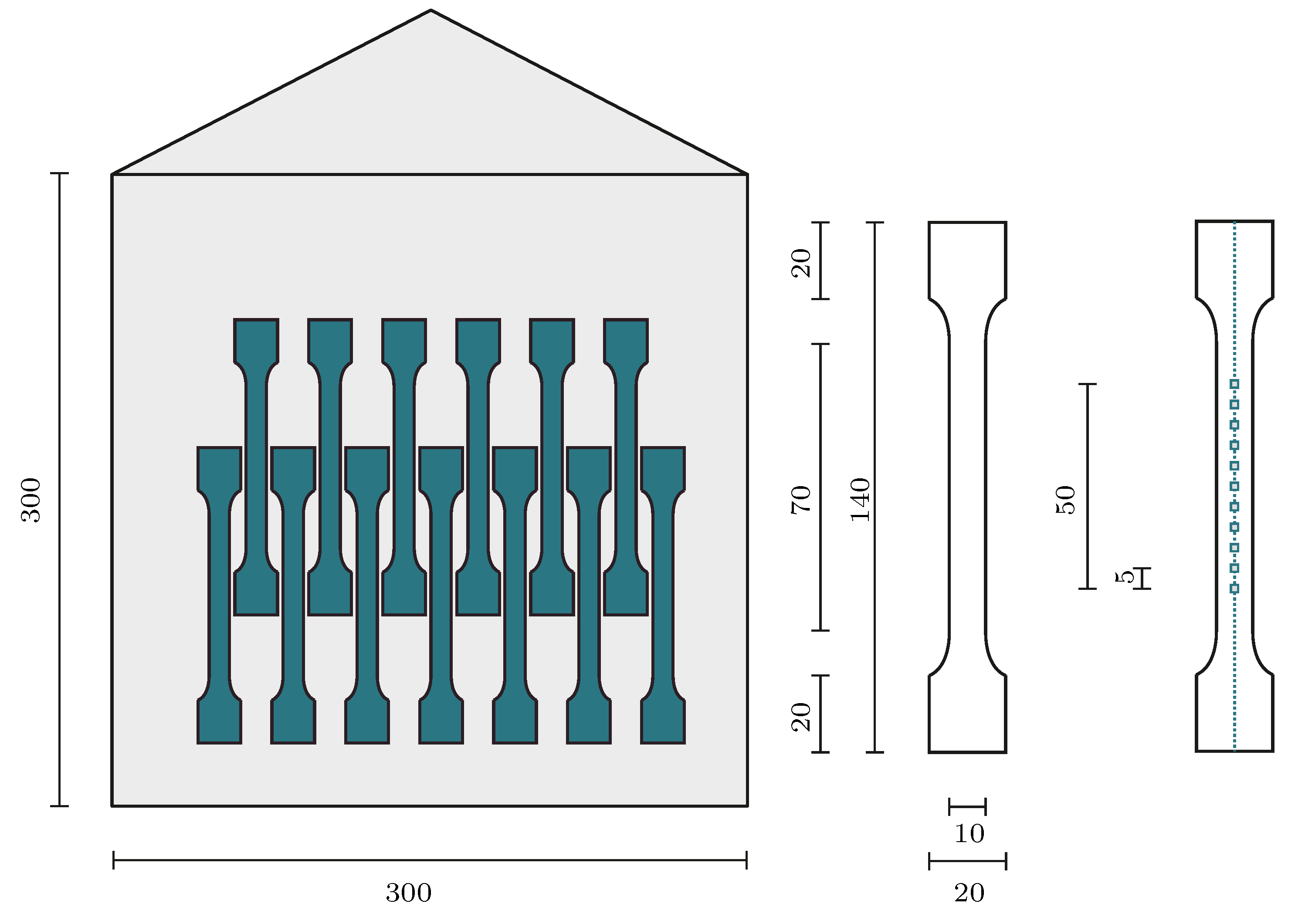
2.1. Specimens
2.2. Experimental Setup and Procedure
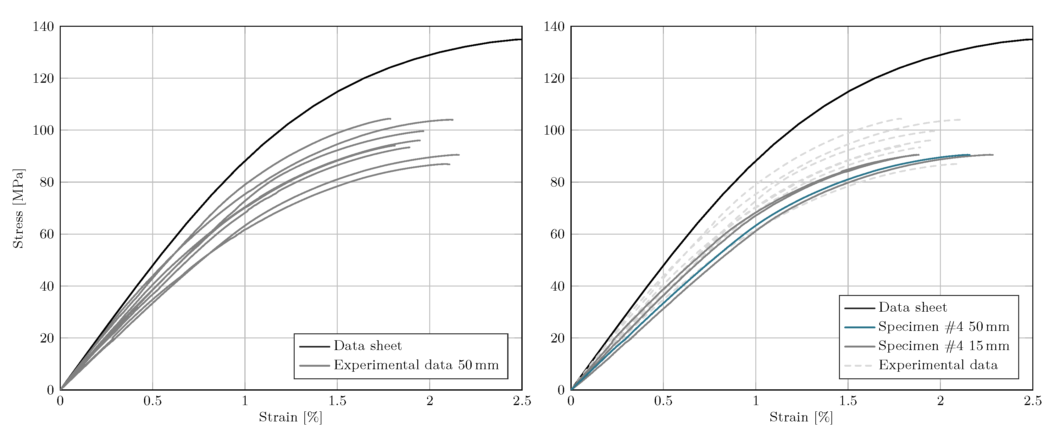
2.3. Results
3. Generation of Cross-Correlated Random Fields
3.1. Methodology
3.1.1. Random Fields
3.1.2. Generation of Random Fields by Numerical Methods
3.1.3. Cross-Correlated Random Fields
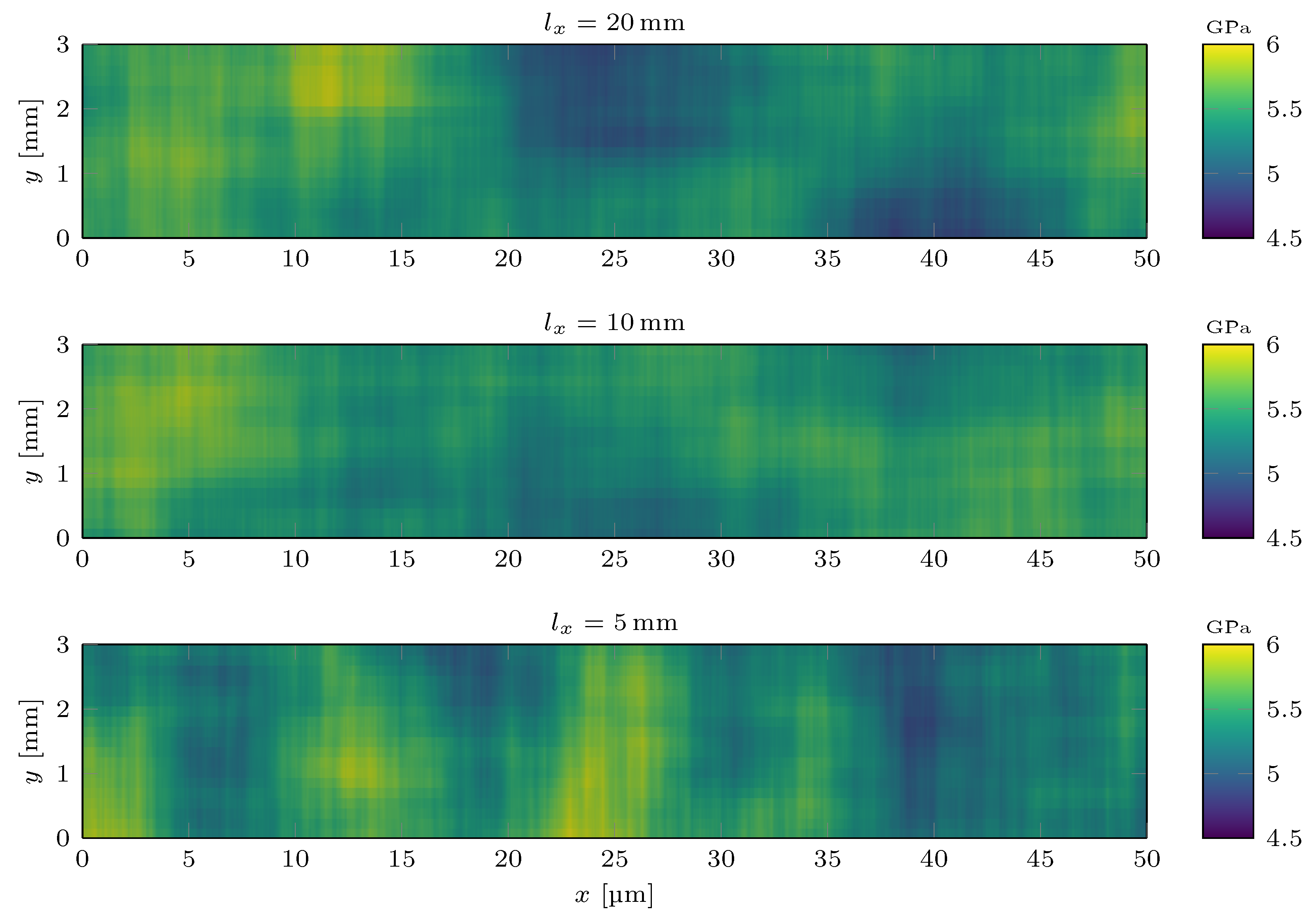
3.2. Application to the Elastic–Ideal Plastic Material Behavior of SFRCs
4. Numerical Simulation
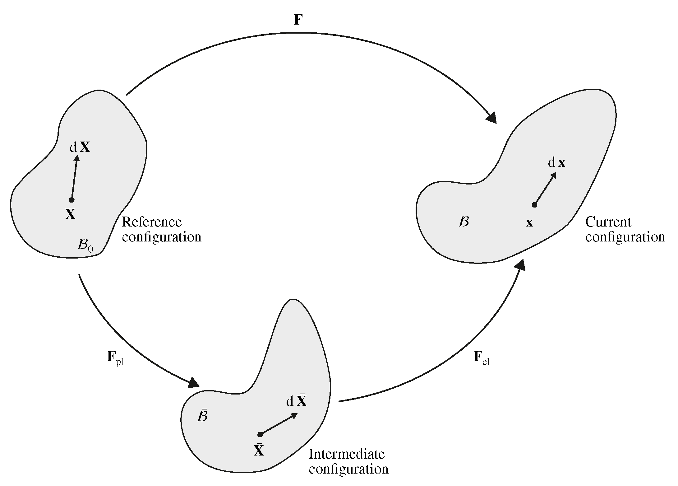
4.1. Framework of Elastic-Ideal Plastic Material Behavior
4.1.1. Constitutive Equations
- Elastic constitutive equation;
- Flow rule;
- Yield condition.
4.1.2. Solution Procedure
Elastic Predictor
Checking Yield Condition
Plastic Corrector Step (Return Mapping)
Updating
4.1.3. Variational Formulation and Consistent Tangent Modulus Tensor
4.2. Implementation in COMSOL Multiphysics®
4.2.1. Algorithm
| Algorithm 1 Main routine implemented in COMSOL Multiphysics® for the calculation of and . |
|
| Algorithm 2 Return mapping algorithm implemented in COMSOL Multiphysics® for the calculation of and . |
Input: see Table 5 Output: see Table 5
|
4.2.2. Validation of the Algorithm
5. Application to Tensile Test Specimen
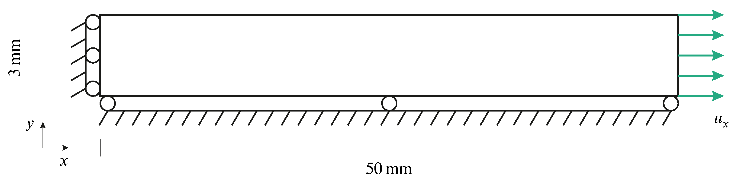
5.1. Numerical Model
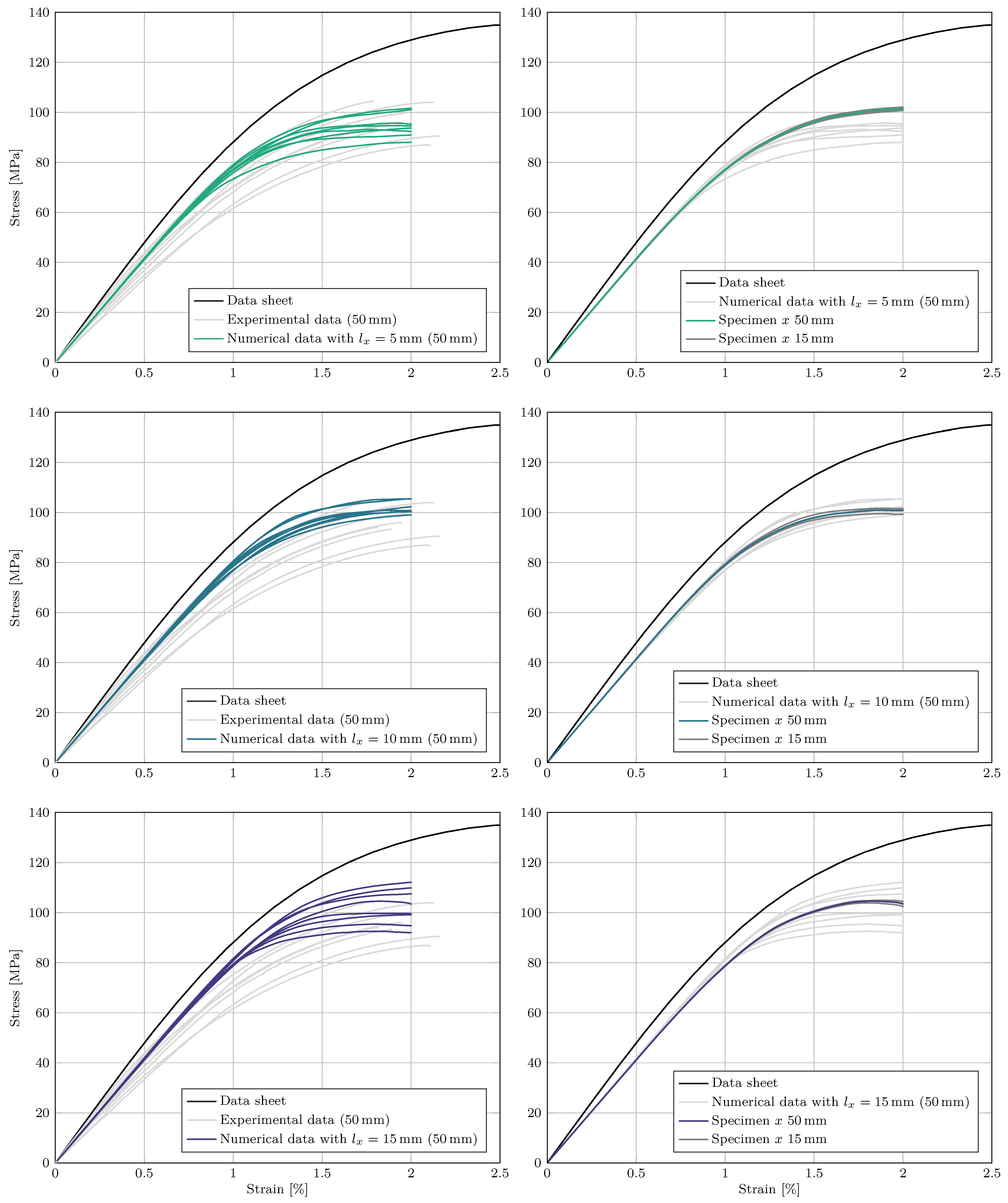
5.2. Results
5.3. Discussion
6. Summary and Conclusions
Funding
Institutional Review Board Statement
Informed Consent Statement
Data Availability Statement
Acknowledgments
Conflicts of Interest
Abbreviations
| DIN | German Institute for Standardization |
| EOLE | Expansion optimal linear estimate |
| FEM | Finite element method |
| ISO | International Organization for Standardization |
| KLE | Karhunen–Loève expansion |
| mcKL | Multiple correlated Karhunen–Loève expansion |
| muKL | Multiple uncorrelated Karhunen–Loève expansion |
| PBT | Polybutylene terephthalate |
| RVE | Representative volume element |
| SFRC | Short fiber-reinforced composite |
| std | Standard deviation |
Appendix A

| Variable | Symbol | Description |
|---|---|---|
| Cel | Input: elastic part of the right Cauchy–Green tensor | |
| lam | Input: material parameter | |
| mu | Input: material parameter | |
| alpha | Input: material parameter | |
| beta | Input: material parameter | |
| gamma | Input: material parameter | |
| tol_inv | − | Input: tolerance for numerical matrix inversion |
| S | Output: second Piola–Kirchhoff stress tensor with respect to the intermediate configuration |
| Variable | Symbol | Description |
|---|---|---|
| F | Input: Deformation gradient | |
| Fpl | Input: plastic part of the deformation gradient | |
| Mdev | Input: deviatoric part of Mandel stress with respect to the intermediate configuration | |
| lam | Input: material parameter | |
| mu | Input: material parameter | |
| alpha | Input: material parameter | |
| beta | Input: material parameter | |
| gamma | Input: material parameter | |
| tol_inv | − | Input: tolerance for numerical matrix inversion |
| dnormx | Output: norm of deviatoric part of Mandel stress with respect to the intermediate configuration |
| Variable | Symbol | Description |
|---|---|---|
| dp | Input: plastic multiplier | |
| F | Input: deformation gradient | |
| Fpl | Input: plastic part of the deformation gradient | |
| lam | Input: material parameter | |
| mu | Input: material parameter | |
| alpha | Input: material parameter | |
| beta | Input: material parameter | |
| gamma | Input: material parameter | |
| sigYs | Input: yield stress | |
| dev | Output: value of the yield function |
| Variable | Symbol | Description |
|---|---|---|
| nmax | − | Input: maximum number of terms of the series representation |
| etol | − | Input: convergence tolerance |
| a | − | Input: matrix |
| aexp | − | Output: tensor exponential function |
| Algorithm A1 Subroutine implemented in COMSOL Multiphysics® for the calculation of . |
| Algorithm A2 Subroutine implemented in COMSOL Multiphysics® for the calculation of |
| Algorithm A3 Subroutine implemented in COMSOL Multiphysics® for the evaluation of . |
| Algorithm A4 Subroutine implemented in COMSOL Multiphysics® for the calculation of the tensor exponential function, adapted from Hashiguchi et al. [55]. |
|
References
- Ebrahimi, F.; Dabbagh, A. A comprehensive review on modeling of nanocomposite materials and structures. J. Comput. Appl. Mech. 2019, 50, 197–209. [Google Scholar]
- Rauter, N. A computational modeling approach based on random fields for short fiber-reinforced composites with experimental verification by nanoindentation and tensile tests. Comput. Mech. 2021, 67, 699–722. [Google Scholar] [CrossRef]
- Hristopulos, D.T. Random Fields for Spatial Data Modeling: A Primer for Scientists and Engineers; Advances in Geographic Information Science; Springer: Dordrecht, The Netherlands, 2020. [Google Scholar]
- Maccone, C. Deep Space Flight and Communications: Exploiting the Sun as a Gravitational Lens; Springer Praxis Books; Springer: Berlin/Heidelberg, Germany, 2009. [Google Scholar]
- Vanmarcke, E. Random Fields: Analysis and Synthesis, Rev. and Expanded New Ed. ed.; World Scientific Publ: Singapore, 2010. [Google Scholar]
- Soize, C. Non-Gaussian positive-definite matrix-valued random fields for elliptic stochastic partial differential operators. Comput. Methods Appl. Mech. Eng. 2006, 195, 26–64. [Google Scholar] [CrossRef] [Green Version]
- Soize, C. Tensor-valued random fields for meso-scale stochastic model of anisotropic elastic microstructure and probabilistic analysis of representative volume element size. Probabilistic Eng. Mech. 2008, 23, 307–323. [Google Scholar] [CrossRef] [Green Version]
- Guilleminot, J.; Soize, C.; Kondo, D.; Binetruy, C. Theoretical framework and experimental procedure for modelling mesoscopic volume fraction stochastic fluctuations in fiber reinforced composites. Int. J. Solids Struct. 2008, 45, 5567–5583. [Google Scholar] [CrossRef] [Green Version]
- Guilleminot, J.; Soize, C.; Kondo, D. Mesoscale probabilistic models for the elasticity tensor of fiber reinforced composites: Experimental identification and numerical aspects. Mech. Mater. 2009, 41, 1309–1322. [Google Scholar] [CrossRef] [Green Version]
- Le, T.T.; Guilleminot, J.; Soize, C. Stochastic continuum modeling of random interphases from atomistic simulations. Application to a polymer nanocomposite. Comput. Methods Appl. Mech. Eng. 2016, 303, 430–449. [Google Scholar] [CrossRef] [Green Version]
- Guilleminot, J.; Soize, C. Non-Gaussian Random Fields in Multiscale Mechanics of Heterogeneous Materials. In Encyclopedia of Continuum Mechanics; Altenbach, H., Öchsner, A., Eds.; Springer: Berlin/Heidelberg, Germany, 2017; pp. 1–9. [Google Scholar] [CrossRef]
- Chen, G.; Suo, X. Constitutive modeling of nonlinear compressive behavior of fiber reinforced polymer composites. Polym. Compos. 2020, 41, 182–190. [Google Scholar] [CrossRef]
- de Groof, V.; Oberguggenberger, M.; Haller, H.; Degenhardt, R.; Kling, A. A case study of random field models applied to thin-walled composite cylinders in finite element analysis. In Proceedings of the 11th International Conference on Structural Safety & Reliability, New York, NY, USA, 16–20 June 2013. [Google Scholar]
- Stefanou, G.; Savvas, D.; Metsis, P. Random Material Property Fields of 3D Concrete Microstructures Based on CT Image Reconstruction. Materials 2021, 14, 1423. [Google Scholar] [CrossRef]
- Zimmermann, E.; Eremin, A.; Lammering, R. Analysis of the continuous mode conversion of Lamb waves in fiber composites by a stochastic material model and laser vibrometer experiments. GAMM-Mitteilungen 2018, 41, e201800001. [Google Scholar] [CrossRef]
- Zheng, K.; Yang, K.; Shi, J.; Yuan, J.; Zhou, G. Innovative methods for random field establishment and statistical parameter inversion exemplified with 6082-T6 aluminum alloy. Sci. Rep. 2019, 9, 17788. [Google Scholar] [CrossRef] [PubMed] [Green Version]
- Huang, H.B.; Huang, Z.M. Micromechanical prediction of elastic-plastic behavior of a short fiber or particle reinforced composite. Compos. Part Appl. Sci. Manuf. 2020, 134, 105889. [Google Scholar] [CrossRef]
- Rauter, N.; Lammering, R. Experimental Characterization of Short Fiber-Reinforced Composites on the Mesoscale by Indentation Tests. Appl. Compos. Mater. 2021, 28, 1747–1765. [Google Scholar] [CrossRef]
- Savvas, D.; Stefanou, G.; Papadrakakis, M. Determination of RVE size for random composites with local volume fraction variation. Comput. Methods Appl. Mech. Eng. 2016, 305, 340–358. [Google Scholar] [CrossRef]
- Breuer, K.; Stommel, M. RVE modelling of short fiber reinforced thermoplastics with discrete fiber orientation and fiber length distribution. SN Appl. Sci. 2020, 2, 140. [Google Scholar] [CrossRef] [Green Version]
- Breuer, K.; Stommel, M. Prediction of Short Fiber Composite Properties by an Artificial Neural Network Trained on an RVE Database. Fibers 2021, 9, 8. [Google Scholar] [CrossRef]
- Zhang, S.; van Dommelen, J.A.W.; Govaert, L.E. Micromechanical Modeling of Anisotropy and Strain Rate Dependence of Short-Fiber-Reinforced Thermoplastics. Fibers 2021, 9, 44. [Google Scholar] [CrossRef]
- Jia, D.; Shi, H.; Cheng, L. Multiscale thermomechanical modeling of short fiber-reinforced composites. Sci. Eng. Compos. Mater. 2017, 24, 765–772. [Google Scholar] [CrossRef]
- Rauter, N. Correlation analysis of the elastic–ideal plastic material behavior of short fiber-reinforced composites. Int. J. Numer. Methods Eng. 2022, 2022, 1–19. [Google Scholar] [CrossRef]
- Baxter, S.C.; Graham, L.L. Characterization of Random Composites Using Moving-Window Technique. J. Eng. Mech. 2000, 126, 389–397. [Google Scholar] [CrossRef]
- Graham-Brady, L.L.; Siragy, E.F.; Baxter, S.C. Analysis of Heterogeneous Composites Based on Moving-Window Techniques. J. Eng. Mech. 2003, 129, 1054–1064. [Google Scholar] [CrossRef]
- Ponte Castañeda, P. The effective mechanical properties of nonlinear isotropic composites. J. Mech. Phys. Solids 1991, 39, 45–71. [Google Scholar] [CrossRef]
- Ponte Castañeda, P. Stationary variational estimates for the effective response and field fluctuations in nonlinear composites. J. Mech. Phys. Solids 2016, 96, 660–682. [Google Scholar] [CrossRef] [Green Version]
- Chemie Wirtschaftsförderungsgesellschaft mbH. CAMPUS® Datasheet: Ultradur® B 4300 G6-PBT-GF30. 2021. Available online: https://www.campusplastics.com/material/pdf/140403/UltradurB4300G6?sLg=en (accessed on 25 June 2021).
- International Organization for Standardization. Plastics–Determination of Tensile Properties: Part 1: General Principles, ISO 527-1:2019 ed.; International Organization for Standardization: Geneva, Switzerland, 2019. [Google Scholar]
- Ghanem, R.G. Stochastic Finite Elements: A Spectral Approach; Springer: New York, NY, USA, 2012. [Google Scholar]
- Sudret, B.; Der Kiurghian, A. Stochastic Finite Element Methods and Reliability: A State-of-the-Art Report; Report No. ucb/semm-2000/08; University of California: Berkeley, CA, USA, 2000. [Google Scholar]
- Chu, S.; Guilleminot, J. Stochastic multiscale modeling with random fields of material properties defined on nonconvex domains. Mech. Res. Commun. 2019, 97, 39–45. [Google Scholar] [CrossRef]
- Guilleminot, J. 12-Modeling non-Gaussian random fields of material properties in multiscale mechanics of materials. In Uncertainty Quantification in Multiscale Materials Modeling; Wang, Y., McDowell, D.L., Eds.; Elsevier Series in Mechanics of Advanced Materials; Woodhead Publishing: Cambridge, UK, 2020; pp. 385–420. [Google Scholar] [CrossRef]
- Malyarenko, A.; Ostoja-Starzewski, M. A Random Field Formulation of Hooke’s Law in All Elasticity Classes. J. Elast. 2017, 127, 269–302. [Google Scholar] [CrossRef] [Green Version]
- Tran, V.P. Stochastic Modeling of Random Heterogeneous Materials. Ph.D. Dissertation, Université Paris-Est, Paris, France, 2016. [Google Scholar]
- Der Kiureghian, A.; Ke, J.B. The stochastic finite element method in structural reliability. Probabilistic Eng. Mech. 1988, 3, 83–91. [Google Scholar] [CrossRef]
- Yamazaki, F.; Member, A.; Shinozuka, M.; Dasgupta, G. Neumann Expansion for Stochastic Finite Element Analysis. J. Eng. Mech. 1988, 114, 1335–1354. [Google Scholar] [CrossRef]
- Vanmarcke, E.; Grigoriu, M. Stochastic Finite Element Analysis of Simple Beams. J. Eng. Mech. 1983, 109, 1203–1214. [Google Scholar] [CrossRef]
- Liu, W.K.; Belytschko, T.; Mani, A. Random field finite elements. Int. J. Numer. Methods Eng. 1986, 23, 1831–1845. [Google Scholar] [CrossRef]
- Liu, P.L.; Kiureghian, A.D. Finite Element Reliability of Geometrically Nonlinear Uncertain Structures. J. Eng. Mech. 1991, 117, 1806–1825. [Google Scholar] [CrossRef]
- Kamiński, M.; Kleiber, M. Stochastic structural interface defects in fiber composites. Int. J. Solids Struct. 1996, 33, 3035–3056. [Google Scholar] [CrossRef]
- Lawrence, M.A. Basis random variables in finite element analysis. Int. J. Numer. Methods Eng. 1987, 24, 1849–1863. [Google Scholar] [CrossRef]
- Spanos, P.D.; Ghanem, R. Stochastic Finite Element Expansion for Random Media. J. Eng. Mech. 1989, 115, 1035–1053. [Google Scholar] [CrossRef]
- Loève, M. Probability Theory, 4th ed.; Springer: New York, NY, USA, 1977; Volume 45. [Google Scholar]
- Cho, H.; Venturi, D.; Karniadakis, G.E. Karhunen–Loève expansion for multi-correlated stochastic processes. Probabilistic Eng. Mech. 2013, 34, 157–167. [Google Scholar] [CrossRef]
- Betz, W.; Papaioannou, I.; Straub, D. Numerical methods for the discretization of random fields by means of the Karhunen–Loève expansion. Comput. Methods Appl. Mech. Eng. 2014, 271, 109–129. [Google Scholar] [CrossRef]
- Ostoja-Starzewski, M. Microstructural Randomness and Scaling in Mechanics of Materials; Chapman and Hall/CRC: New York, NY, USA, 2007. [Google Scholar] [CrossRef]
- Li, C.C.; Der Kiureghian, A. Optimal Discretization of Random Fields. J. Eng. Mech. 1993, 119, 1136–1154. [Google Scholar] [CrossRef]
- Atkinson, K.E. The Numerical Solution of Integral Equations of the Second Kind; Cambridge University Press: Cambridge, UK, 2010. [Google Scholar] [CrossRef] [Green Version]
- Rauter, N.; Lammering, R. Correlation structure in the elasticity tensor for short fiber-reinforced composites. Probabilistic Eng. Mech. 2020, 62, 103100. [Google Scholar] [CrossRef]
- Golub, G.H.; van Loan, C.F. Matrix Computations; Johns Hopkins Studies in the Mathematical Sciences; Johns Hopkins Univ. Press: Baltimore, MD, USA, 2007. [Google Scholar]
- Ghanem, R.G.; Spanos, P.D. Polynomial Chaos in Stochastic Finite Elements. J. Appl. Mech. 1990, 57, 197–202. [Google Scholar] [CrossRef]
- Simo, J.C.; Hughes, T.J.R. Computational Inelasticity. In Interdisciplinary Applied Mathematics; Springer: New York, NY, USA, 1998; Volume 7. [Google Scholar]
- Hashiguchi, K. Introduction to Finite Strain Theory for Continuum Elasto-Plasticity, Online-Ausg ed.; Wiley Series in Computational Mechanics; Wiley: Chichester, UK, 2012. [Google Scholar]
- Eidel, B.; Gruttmann, F. Elastoplastic orthotropy at finite strains: Multiplicative formulation and numerical implementation. Comput. Mater. Sci. 2003, 28, 732–742. [Google Scholar] [CrossRef]
- Bonet, J.; Burton, A.J. A simple orthotropic, transversely isotropic hyperelastic constitutive equation for large strain computations. Comput. Methods Appl. Mech. Eng. 1998, 162, 151–164. [Google Scholar] [CrossRef]
- Kröner, E. Allgemeine Kontinuumstheorie der Versetzungen und Eigenspannungen. Arch. Ration. Mech. Anal. 1959, 4, 273–334. [Google Scholar] [CrossRef]
- Lee, E.H.; Liu, D.T. Finite–Strain Elastic–Plastic Theory with Application to Plane–Wave Analysis. J. Appl. Phys. 1967, 38, 19–27. [Google Scholar] [CrossRef]
- Lee, E.H. Elastic-Plastic Deformation at Finite Strains. J. Appl. Mech. 1969, 36, 1–6. [Google Scholar] [CrossRef]
- Mandel, J. Director vectors and constitutive equations for plastic and visco-plastic media. In Problems of Plasticity; Sawczuk, A., Ed.; Springer: Dordrecht, The Netherlands, 1974; Volume 4, pp. 135–143. [Google Scholar] [CrossRef]
- Lubarda, V.A. Elastoplasticity Theory; CRC PRESS: Boca Raton, FL, USA, 2019. [Google Scholar]
- Vladimirov, I.N.; Pietryga, M.P.; Reese, S. On the modelling of non–linear kinematic hardening at finite strains with application to springback—Comparison of time integration algorithms. Int. J. Numer. Methods Eng. 2008, 75, 1–28. [Google Scholar] [CrossRef]
- Miehe, C. Exponential map algorithm for stress updates in anisotropic multiplicative elastoplasticity for single crystals. Int. J. Numer. Methods Eng. 1996, 39, 3367–3390. [Google Scholar] [CrossRef]
- Simo, J.C.; Ortiz, M. A unified approach to finite deformation elastoplastic analysis based on the use of hyperelastic constitutive equations. Comput. Methods Appl. Mech. Eng. 1985, 49, 221–245. [Google Scholar] [CrossRef]
- Simo, J.C. A framework for finite strain elastoplasticity based on maximum plastic dissipation and the multiplicative decomposition. Part II: Computational aspects. Comput. Methods Appl. Mech. Eng. 1988, 68, 1–31. [Google Scholar] [CrossRef]
- Simo, J.C. A framework for finite strain elastoplasticity based on maximum plastic dissipation and the multiplicative decomposition: Part I. Continuum formulation. Comput. Methods Appl. Mech. Eng. 1988, 66, 199–219. [Google Scholar] [CrossRef]
- Altenbach, H. Kontinuumsmechanik; Springer: Berlin/Heidelberg, Germany, 2015. [Google Scholar] [CrossRef]
- Malvern, L.E. Introduction to the Mechanics of a Continuous Medium; Prentice-Hall Series in Engineering of the Physical Sciences; Prentice-Hall: Englewood Cliffs, NJ, USA, 1969. [Google Scholar]
- Holzapfel, G.A. Nonlinear Solid Mechanics: A Continuum Approach for Engineering, Reprinted with Corrections ed.; John Wiley & Sons Ltd.: Chichester, Switzerland; Weinheim, Germany; New York, NY, USA; Brisbane, Australia; Singapore; Toronto, ON, Canada, 2000. [Google Scholar]
- Spencer, A.J.M. Deformations of Fibre-Reinforced Materials; Oxford Science Research Papers; Clarendon Press: Oxford, UK, 1972. [Google Scholar]
- Miehe, C. Numerical computation of algorithmic (consistent) tangent moduli in large-strain computational inelasticity. Comput. Methods Appl. Mech. Eng. 1996, 134, 223–240. [Google Scholar] [CrossRef]
- Menzel, A.; Steinmann, P. On the spatial formulation of anisotropic multiplicative elasto-plasticity. Comput. Methods Appl. Mech. Eng. 2003, 192, 3431–3470. [Google Scholar] [CrossRef]
- Menzel, A.; Ekh, M.; Runesson, K.; Steinmann, P. A framework for multiplicative elastoplasticity with kinematic hardening coupled to anisotropic damage. Int. J. Plast. 2005, 21, 397–434. [Google Scholar] [CrossRef]
- Belytschko, T.; Liu, W.K.; Moran, B. Nonlinear Finite Elements for Continua and Structures, Repr ed.; Wiley: Chichester, UK, 2003. [Google Scholar]
- Rauter, N.; Lammering, R. The impact of fiber properties on the material coefficients of short fiber-reinforced composites. PAMM 2020, 20, e202000019. [Google Scholar] [CrossRef]
- Gandhi, U.N.; Goris, S.; Osswald, T.A.; Song, Y.Y. Discontinuous Fiber-Reinforced Composites: Fundamentals and Applications; Hanser Publishers and Hanser Publications: Munich, Germany; Cincinnati, OH, USA, 2020. [Google Scholar]
- Rolland, H.; Saintier, N.; Robert, G. Fatigue Mechanisms Description in Short Glass Fiber Reinforced Thermoplastic by Microtomographic Observation. In Proceedings of the 20th International Conference on Composite Material, Copenhagen, Denmark, 19–24 July 2015. [Google Scholar]
- Structural Mechanics Module User’s Guide; COMSOL Multiphysics® v. 5.5; COMSOL AB: Stockholm, Schweden, 2019.


| E | |||||||
|---|---|---|---|---|---|---|---|
| Specimens | Number of Specimens | mean | sth | mean | sth | mean | sth |
| Gpa | Gpa | MPa | MPa | % | % | ||
| Experiments | 8 | 7.95 | 0.87 | 96.1 | 6.22 | 1.97 | 0.14 |
| Data sheet | 1 | 9.69 | - | 135 | - | 2.5 | - |
| Parameter | Mean | Standard Deviation | Correlation Function | Correlation Length Ratio |
|---|---|---|---|---|
| GPa | GPa | - | ||
| 5.38 | 0.140 | Triangle | 1 | |
| 1.20 | 0.064 | Exponential | 0.4 | |
| 1.10 | 0.090 | Exponential | 0.4 | |
| −0.13 | 0.020 | Triangle | 1 | |
| 1.13 | 0.148 | Triangle | 1 | |
| 0.126 | 0.015 | Triangle | 1 |
| Variable | Symbol | Description |
|---|---|---|
| FlOld | Input: deformation gradient at previous step | |
| Fl | Input: deformation gradient at current step | |
| tempOld | Input: temperature at previous step | |
| temp | Input: temperature at current step | |
| K | Input: local material coordinate system | |
| delta | − | Input: reserved for future use |
| nPar | n | Input: number of material model parameters |
| par | − | Input: array with the material model parameters |
| sPK | Output: second Piola–Kirchhoff stress tensor given in Voigt order | |
| J | Output: Jacobian of the stress with respect to the deformation gradient as a 6-by-9 matrix of partial derivatives of the components of sPK with respect to the components of F |
| Variable | Symbol | Description |
|---|---|---|
| nStates1 | − | Input: size of the state array |
| states1 | Input: plastic part of the deformation gradient at the previous step |
| Variable | Symbol | Description |
|---|---|---|
| F | Input: deformation gradient | |
| Fpl | Input: plastic part of the deformation gradient | |
| Fpl | Output: updated plastic part of the deformation gradient | |
| Sint | Output: second Piola–Kirchhoff stress tensor with respect to the intermediate configuration | |
| lam | Input: material parameter | |
| mu | Input: material parameter | |
| alpha | Input: material parameter | |
| beta | Input: material parameter | |
| gamma | Input: material parameter | |
| sigYs | Input: yield stress |
| GPa | GPa | GPa | GPa | GPa | MPa | |
|---|---|---|---|---|---|---|
| Neo-Hookean | 5.38 | 1.20 | - | - | - | 50 |
| Transversely isotropic | 5.38 | 1.20 | 1.10 | −0.13 | 1.13 | - |
| Strain Level | Experimental Data | |||||||
|---|---|---|---|---|---|---|---|---|
| mean | std | mean | std | mean | std | mean | std | |
| MPa | MPa | MPa | MPa | MPa | MPa | MPa | MPa | |
| 0.2 | 16.6 | 0.1 | 16.6 | 0.1 | 16.6 | 0.1 | 16.1 | 1.8 |
| 0.5 | 41.6 | 0.3 | 41.4 | 0.3 | 41.3 | 0.2 | 38.7 | 3.7 |
| 1.0 | 80.0 | 1.2 | 78.6 | 1.6 | 76.9 | 1.7 | 70.0 | 5.8 |
| 1.5 | 99.2 | 5.2 | 97.7 | 2.6 | 92.0 | 3.9 | 88.5 | 6.8 |
| 2.0 | 102.3 | 7.2 | 101.8 | 2.4 | 94.7 | 4.9 | 95.8 | 6.3 |
Publisher’s Note: MDPI stays neutral with regard to jurisdictional claims in published maps and institutional affiliations. |
© 2022 by the author. Licensee MDPI, Basel, Switzerland. This article is an open access article distributed under the terms and conditions of the Creative Commons Attribution (CC BY) license (https://creativecommons.org/licenses/by/4.0/).
Share and Cite
Rauter, N. Numerical Simulation of the Elastic–Ideal Plastic Material Behavior of Short Fiber-Reinforced Composites Including Its Spatial Distribution with an Experimental Validation. Appl. Sci. 2022, 12, 10483. https://doi.org/10.3390/app122010483
Rauter N. Numerical Simulation of the Elastic–Ideal Plastic Material Behavior of Short Fiber-Reinforced Composites Including Its Spatial Distribution with an Experimental Validation. Applied Sciences. 2022; 12(20):10483. https://doi.org/10.3390/app122010483
Chicago/Turabian StyleRauter, Natalie. 2022. "Numerical Simulation of the Elastic–Ideal Plastic Material Behavior of Short Fiber-Reinforced Composites Including Its Spatial Distribution with an Experimental Validation" Applied Sciences 12, no. 20: 10483. https://doi.org/10.3390/app122010483
APA StyleRauter, N. (2022). Numerical Simulation of the Elastic–Ideal Plastic Material Behavior of Short Fiber-Reinforced Composites Including Its Spatial Distribution with an Experimental Validation. Applied Sciences, 12(20), 10483. https://doi.org/10.3390/app122010483