Abstract
Water is essential for agriculture in many world regions and for achieving sustainability in production systems. Maximizing net returns with the available resources is significant, but doing so is a complex problem, owing to the many factors that affect this process. In this study, a decision support system (DSS) incorporating a crop planning model is developed for identifying optimal cropping plans and irrigation management. The model estimates crop yield, production, water requirement, and net income. In this system, the Simulated Annealing algorithm (SA) is used as an optimization tool inside the DSS developed, and the result is as robust as the exact solution with higher computational efficiency. From the model applied, it is found that the current crop pattern and water distribution plan used in the study area should be improved. The computational analysis also found that of the five plans proposed, three plans could produce the highest generated income. On contrary, the current strategy used by Tak’s province farmer has the lowest generated income. This result shows that if a better-designed and more efficient crop planning method was, should be used instead.
1. Introduction
In Agriculture 1.0, crop yields relied on labor and animals; in Agriculture 2.0, agricultural machinery and chemicals improved crop yields. Agriculture 3.0 uses machines to produce better crops with less energy, more precision, and less environmental damage. Agriculture 4.0 has advanced the way of farming. According to Zecca [1], Agriculture 4.0 focuses on natural resource management, ecosystem conservation, sufficient services, and contemporary technologies to fulfill rising needs. Technology such as Big data, AI, and IoT are meant to increase agricultural efficiency, sustainability, and environmental impact [2]. It has been reported that machine learning, IoT, and AI have improved the agriculture industry in numerous categories, including yield prediction [3,4,5], disease detection [6,7,8], crop recognition [9,10], and water management [11,12,13]. Low-cost sensor-based IoT is developed by Ferrández-Pastor et al. [14] to optimize production efficiency, increase quality, and minimize environmental impacts by optimizing resources such as water and energy. Lately, the smart farming trend also incorporates big data as predictive and operational tools [15]. An application for precision agriculture using cloud technology is beneficial to optimize irrigation management [16].
Agricultural sectors are influenced by a number of factors. Climate change, water availability, soil fertility, and economic variables all have an impact on the agriculture sector [17]. Seasons, as one of the contributing components, have a significant impact on agricultural crop production. A Decision Support System (DSS) can offer a list of suggestions that could assist farmers as decision-makers to achieve better performances with available information. Some existing DSS utilized mathematical optimization in agriculture and concentrated on a single sort of analysis, such as water distribution [16,18,19], land assignment [20,21], weather and climate forecast [22,23], co-learning process in agricultural sector [24], etc. DSS takes in different kinds of information and processes them with models and data to come up with specific recommendations. DSSs can also be designed to support farmers and related parties [22], such as government and farm advisors, based on data availability. However, it is important that the DSS involved stakeholders effectively. The involvement could happen by using simplified models to make informed and timely decisions [25].
Thailand’s agriculture sector provided up to 12 percent of the country’s Gross Domestic Product (GDP) and employed over 30 percent of the country’s whole workforce [26,27]. Rice, cassava, rubber, sugar, corn, and palm oil accounted for around 75 percent of the market value of Thai agriculture. There are currently 23.9 million hectares of cultivable land in use, of which 68 percent is for field crops [28]. Despite the fact that agriculture can employ a substantial proportion of the labor force, it has the lowest value-added per worker compared to other industries. According to United Nations Thailand, there are still a number of challenges that must be addressed in order to improve the performance of Thailand’s agricultural industry, including inefficiencies in small-plot farming, a lack of current technology, and a lack of awareness of contemporary farming techniques [29]. Since most crop farmers are smallholders, it’s possible that the limited resources are not being shared well, which could lead to lower crop productivity. As Thailand has a climate, it only rains about 70 mm on average during the hot season from March to April and 19 mm on average during the cool season from November to February [30]. In the rainy season from May to October, the lowest precipitation is 149 mm and the greatest is 279 mm [30]. Given the limited supply of water, it is necessary to implement a water management and irrigation system to ensure that the crop receives the right amount of water. In Thailand, only two-thirds of farmers have access to irrigation, while one-third do not, according to data obtained by the National Statistical Office (NSO) from the Agricultural census in 2003 and 2013 [31]. According to Attavanich et al. [32], In 2017, 42% of agricultural households and small farmers had access to water resources, 26% through irrigation, 11% from homes, and 6% from natural/public water sources. Temperature increases caused by climate change have a substantial impact on agriculture. Occasionally caused by droughts or floods, unpredictability of the weather makes it more difficult for farmers to reap a successful harvest. Consequently, the climate change element should also be assessed for future improvements, since the use of increased water in conjunction with enhanced fertilization management could result in essential agricultural production benefits.
Farmers and related stakeholders may face a number of obstacles while attempting to make the best selections from the vast array of available options. A DSS must be meticulously created with consideration for numerous criteria, employing well-defined data and a tool capable of transforming the data into a set of relevant recommendations. Farmers and the agricultural system will benefit from the development of DSS and mathematical optimization to determine the optimal crop planning and irrigation scheduling in respect of water availability. Consequently, the purpose of this work is to provide an integrated optimization scheduling DSS for farmers and related stakeholders to assist farmers and related stakeholders in making decisions based on evidence. For each module, farmers or decision-makers will select the optimal solutions, based on their future perspectives and experiences. As water availability and distribution are the primary focus of this study, the DSS includes an optimization module that matches crop type and water availability based on the availability of water. The results of the DSS will not provide farmers or decision-makers with clear instructions or directions. In this instance, farmers are in a position to make the final decisions. The agriculture system in Thailand’s Tak Province is analyzed, and the DSS is offered to increase the system’s efficiency.
The remainder of the paper is organized as follows. In Section 2, we describe the DSS theoretical framework. The proposed method that incorporates solving the model is introduced in Section 3, for which the agriculture as study case and DSS capabilities are illustrated in Section 4. Section 4 also discusses the managerial implications, and Section 5 discusses the main findings and future lines of research.
2. Theoretical Framework
This study aims to help farmers deal with certain issues that potentially give a long-term benefit to yield better agricultural production. Based on the literature review and field survey, the farmers of Tak Province are dealing with the following issues: (1) Limited water availability during hot season hinders the optimal yield of the crop; (2) variability of the crop, which requires a different amount of water. As some small farmers raised issues mostly about water availability, a DSS was developed. In summary, the DSS will be focused on crop planning and water distribution/irrigation management.
2.1. Indices and Parameters
= Crop i
= The irrigation zones
= Number of crops
= Number of crop zones
= The total area of the crop planted in each zone z (m2)
= The price of crop i (baht/Kg)
= The fixed production cost of crop i (baht/Kg)
= The cycle of crop i per year
= Crop yield (a measurement of the amount of agricultural production harvested per unit of land area) (Kg/m2)
= The upper bound of the total area of crop i (%) in the area z
= The lower bound of the total area of crop i (%) in the area z
= Crop Coefficient of crop i
= Reference Crop Evapotranspiration (mm. per day) in month m
= If crop i is planted in month m = {1, 2, 3, …, 12}
= Number of days in each month (Days)
= Amount of water available in each month (m3)
2.2. Decision Variables
= Total water for crop i in month m (mm)
= Total area of the crop i planted in zone z (m2)
= Total water of zone z in month m (m3)
= Total water in month m (m3)
The problem maximizes the net economic benefit and crop area under the available water in the irrigation zones (z). Each crop (i) can be described as a gross margin (yields and prices).
| (1) | ||
| for all m = {1, 2, …, 12}, i = {1, 2, …,N} | (2) | |
| for all z = {1, 2, …, M}, m = {1, 2, …, 12} | (3) | |
| for all m = {1, 2, …, 12} | (4) | |
| for all z = {1, 2, …, M} | (5) | |
| for all m = {1, 2, …, 12} | (6) | |
| for all i = {1, 2, …, N} | (7) | |
| for all i = {1, 2, …, N} | (8) |
Objective (1) proposes a function for maximizing the net return for crop planning. Constraint (2) calculates the total water for each crop in each month. The crop coefficients Kc are generated using Penman–Monteith method [33,34]. Constraints (3) and (4), the amount of water distribution for each zone in each month is evaluated. Constraint (5) ensures that the total cropping area must not exceed the total irrigation area. Constraint (6) ensures that the total volume of water applied each year must not exceed the corresponding available supply. Constraints (7) and (8) are used to limit the crop area.
3. Proposed Methodology
The DSS development process was developed to ensure that decision-makers which are farmers and related stakeholders, could use and understand it easily. A DSS prototype with a complete graphical user interface (GUI) was developed with system functionality developed in parallel with the solution solver. All methodologies are coded using MATLAB. The Basic DSS Module for this study is shown in Figure 1.
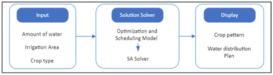
Figure 1.
The Basic DSS Module for Tak Agriculture.
3.1. Case Study
The agricultural sector in Thailand is mainly located in the northern part of the country, with Tak City as one of the agricultural areas. Tak City is the capital of Tak Province, situated in western Thailand, 492 km from Bangkok. One of their primary industries is the agricultural sector. According to data from the Central Agricultural Registration Database System of the Ministry of Agricultural Extension in 2020, the top five products produced in Tak City are corn, rice, cane, cassava, and rubber, as shown in Figure 2 [35]. Tak has a tropical savanna climate, where winter is dry and warm, and summer can reach up to 37 °C [36]. The average rainfall throughout the last decades has been varied, with the highest during July and August, as shown in Figure 3. As part of its development, the need to have better farming management in Tak City increases. In the Tak City case, some agricultural products are not rainfed and depend much on irrigation water. That being said, irrigation management is needed to enhance the productivity of small farmers and ensure that those small farmers can gain access to water resources.
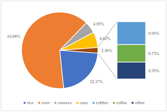
Figure 2.
Tak City Agriculture Product Yield Percentage in 2020 (Plotted from Central Agricultural Registration Database System Ministry of Agricultural Economics Thailand, 2020 [35]).
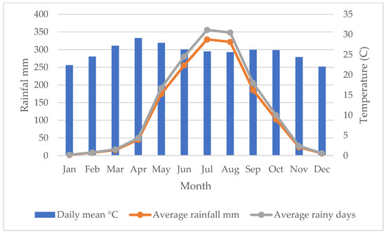
Figure 3.
Average Monthly Precipitation and Temperature (1981–2010) (Plotted from: Thai Meteorological Department, 2018 [36]).
Irrigation management aims to give the proper amount of water to the crop according to their necessity. Irrigation management should yield both quality and quantity of the crops based on the type of crop, type of soil, and water availability. The timing for water irrigation is also important to achieve optimum production. Nonetheless, the need for better agriculture management is not limited to only irrigation management. Due to climate changes, the rainy season period is shifted, and thus analytical water forecasting needs to be conducted before planting the crop. The result of the water forecast also helps the type of crop that should be planted and how the water should be distributed, respectively. The type of soil and water availability can help farmers decide the type of crop they will plant in certain areas. Nevertheless, as the problems lie in the limitation of soil nutrients and water for better crop yields, the decision support system (DSS) is needed to manage and optimize those limitations.
In Tak province, Huay Mae Thor reservoir withholds 63,000,000 m3 and supplies water for many uses, especially agriculture. This amount of water can provide about 51,200,000 m2 of agricultural area. However, only 6,640,800 m2 are provided by the reservoir. Six gates connecting the river and the reservoir control the water to the agricultural area in six zones shown in Figure 4. The average amount of water from 2016 to 2020 is about 42,000,000 m3, illustrated in Figure 5. The DSS is applied to crop planning and irrigation management in the case study of Huay Mae Thor reservoir, Tak Province, Thailand. Six areas/zones are considered in the experiment, where the water from the reservoir is supplied to the agricultural area shown in Table 1.
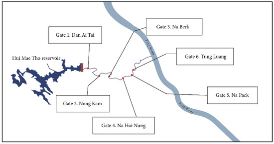
Figure 4.
The location of six gates connecting Ping River and Hui Mae Tho Reservoir.
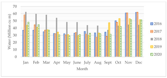
Figure 5.
Average water available per month from Hui Mae Tho Reservoir (2016–2020).

Table 1.
The agricultural area in Tak Province supplied with water from Hui Mae Tho Reservoir.
3.2. Heuristics Algorithm in DSS
In this study, we proposed Simulated Annealing (SA) to solve the optimization and scheduling model in DSS. This methodology is chosen due to its robustness and has been proven to yield fast and nearly optimum results in many optimization problems [37,38,39,40,41,42,43]. SA belongs to a single solution-based search; for each iteration, its focus is on modifying a single candidate solution to achieve a better solution. In the present study, the SA algorithm consists of three phases: random generation of an initial solution, improvement of the initial solution using three neighborhood moves, and calculation of the objective value. The following subsection discusses the algorithm in detail.
3.2.1. Solution Representation
Figure 6 presents the solution representation used in this study corresponding to the type of crop (i) assigned to each zone (z). For each planting zone/area, there will be different solution representations. Furthermore, the initial solution is generated by assigning a permutation of a randomly generated sequence at each zone. In other words, the sequence represents the priority of the crop to be planted at each zone. This initial random solution procedure might have an infeasible assignment of crop type to a particular zone. Thus, this condition is repaired by neglecting the infeasible assignment and continuously considering the next available crop option in the associated sequence.
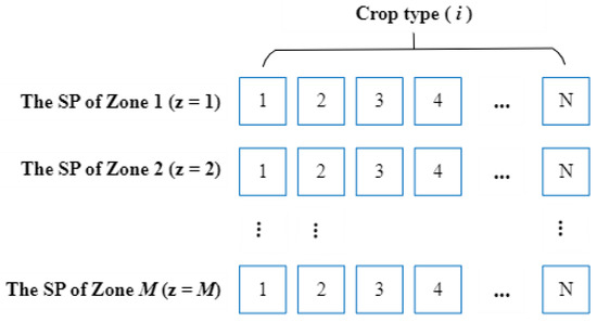
Figure 6.
Solution Representation (SP).
3.2.2. Neighborhood
One out of two neighborhood moves is selected randomly at each iteration to generate a new solution based on the last solution/current solution. The moves are denoted as swap and insert. First, a random zone (z) is selected to apply the move. The swap move is carried out by exchanging the positions of randomly selected two points from the sequence which represent the crop (index i). Meanwhile, an insertion move is applied by randomly selecting two points represented in the crop sequence, namely the kth and lth positions. Then the crop correspondence to the kth position is inserted after the crop at the jth position. The generation of the probability function is taken from a generic choice of uniform distributions with a probability proportional to the size of the neighborhood, which in this study is set to 1/2 proportion for each neighborhood. Note that the neighborhood movement enables the solution to move toward an infeasible solution. The infeasible solution might occur because the total area of crop assigned to a particular zone is not in the range of the total area being preferred, and the total planted area in all zones is more than the area available. This condition is described in detail by the model formulation in constraints (6), (7), and (4). However, the infeasibility of the solution can be easily treated by neglecting the crop assignment that led the solution to infeasibility. Thus, the solution will remain a feasible solution despite the infeasibility due to the neighborhood movement.
3.2.3. The SA Procedure and Parameters
Algorithm 1 described the procedure of the proposed SA. The proposed SA algorithm requires five parameters: Iiter, T0, Tf, , and K. Iiter denotes the number of iterations with which the search proceeds at a particular temperature. T0 represents the initial temperature. Tf is the final temperature and is a coefficient used to control the speed of the cooling schedule. Finally, K is the Boltzmann constant used to calculate accepting a worse solution.
The proposed SA methodology starts with a random initial solution. Then, the current temperature T is set to the initial temperature T0. The best solution Xbest and the current solution X are the initial solution. The best objective value is set to be the objective value of solution X. The initial probabilities are used at the first temperature.
The process generates a new solution Y from the current solution X using one of the neighborhood’s moves between swap and insert. This process is applied for several iterations at a particular temperature. Let Δ be the objective solution difference between Y and X. In this case, there will be three Δ solutions consisting of Δswap or Δinsert. If Δ > 0, then Y is better than X; thus, Y replaces X as the current solution. Otherwise, the new neighborhood solution is accepted with a probability calculated by the Boltzmann function; The temperature is updated based on the current temperature (T) decreasing to αT. The SA algorithm is terminated if the current temperature is below or equal to the final temperature Tf.
| Algorithm 1. Simulated Annealing Algorithm Procedure |
| 1: Input: Iiter, T0, Tf, , K, 2: Output: Obj; 3: InitialSolution ← Generate randomly; 4: I ← 0; T ← T0; Fbest ← Obj (X), X ← InitialSolution; Xbest ← X; 5: Rt ← 1/3 for all t in {swap, reverse, insert}; 6: While T < Tf; 7: I ← 1; Nt ← 0 and Ot ← Ø for all t in {swap, reverse, insert}; W← 0; 8: While I ≤ Iiter; 9: r ← random (0,1); 10: If (r ≤ 0.5) then 11: Generate a new solution Y from X by random swap neighborhood; 12: Else 13: Generate a new solution Y from X by inserting neighborhood; 14: End if 15: Δ ← obj (Y) − obj (X); 16: If (Δ > 0) then X ← Y; 17: Else r ← random (0, 1); 18: If (r < exp(∆/KT)) then X ← Y; End if 19: End if 20: If (Obj(X) < Fbest) then Xbest ← X; Fbest ← Obj(X); End if 21: I ← I + 1; 22: End while 23: T = T; 24: End while |
4. Computational Results and Discussions
This section is consisting of three parts. First, a crop pattern solution for a particular case is presented. Then, to show the effectiveness of the proposed DSS, a comparison between the solution generated by the exact solution approach and the metaheuristic approach applied in the DSS is presented. Finally, a sensitivity analysis of the results is analyzed based on several scenarios with different availability of crop patterns. Table 2 shows the 15 agricultural products (crops) that can be chosen to be cultivated in each of these zones.
Table 2.
The data of crops cultivated in agricultural areas/zone in Tak Province.
4.1. An Example of Crop Pattern Solution
This sub-section describes an example of a crop pattern solution that might be generated for a particular problem sample. Table 3 shows that each zone has limitations regarding the total area of each crop permitted to be cultivated by having minimum and maximum percentages of it. According to Table 3, Mae Thor 2 (Den Ai Tai), for example, has a limitation considering the total percentage of each crop permitted to be cultivated in the zone. Crop 1 should be cultivated at least 25% of the total area. Crops 2–5 should be cultivated at least 10% of the total area. The rest crops do not have limitations regarding the percentage of the area that needs to be cultivated. This limitation was set based on the consideration of best practices and the economic value of the crop that has been previously gathered.
Table 3.
Minimum and maximum percentages permitted to cultivate crops in each area.
The data shown in Table 3 is used as an input for crop planning and irrigation management based on the proposed mathematical model. The results obtained are displayed in Table 4. The result shows that, In Mae Thor 2, out of the total area of 1,705,600 m2, Crop 1 was planned for cultivation in 426,400 m2 equals 25% of the total area. Crops 2–5 were planned for equal cultivation of 170,560 m2 corresponding to 10% of the total area. Crop 7 was planned for cultivation in 596,960 m2 equals 35% of the total area. These explanations were similar to the result of agricultural planning of another zone shown in Table 4. These plans would generate a maximum agricultural income of 42,110,600 baht/year. They were also the plans for sufficient water utilization in the reservoir. Furthermore, the permitted amounts of water utilized and allocated monthly at each zone are displayed in Table 5.
Table 4.
The results of finding cultivation areas from the mathematical models for suitable agricultural planning.
Table 5.
Expected water amounts of each area in each month.
4.2. Comparison between the Exact Solution and SA
This sub-section describes the comparison of the results between the exact solution approach using an approximation approach of the proposed simulated annealing. The experiments are conducted on 20 samples which consist of data based on Table 1 and Table 2. However, each sample has different minimum and maximum percentages permitted for cultivation in each area, in which the example has been shown previously in Table 3. This experiment aims to test the quality of the solution provided by the exact solution approach compared with SA. The exact solution approach was applied using AMPL, a commercial software package. The solution provided by AMPL was regarded as the optimal solution. However, the exact solution has some limitations. To solve larger size or more complex problems, AMPL may take a longer time to find the answers. Sometimes, it could not even find one. Therefore, in this case, metaheuristics are preferred. In addition, the AMPL software package maybe not be feasible for some decision-makers due to investment costs that need to be applied if the application is going to be used for commercial purposes.
Table 6 shows that SA can find the exact solution generated by AMPL. However, it may take a longer time to solve the problem. This is suspected because the size of instances available to use for the experiment is still considerably small. In more detail, AMPL can report the optimal solution on an average of 2.40 s. Meanwhile, SA requires an average of 6.95 s to report the optimal solution. Despite SA reportedly taking a long time to generate the solution, this study still encourages the use of SA for further experiments. First, the time difference to solve the problem is still considered reasonable. Second, it is due to the consideration of practical delivery of the DSS to the stakeholder that the use of AMPL will require the decision-maker to have another investment in the software to be able to use it for a commercial purpose.
Table 6.
Comparison between AMPL and SA.
4.3. Crop Pattern Scenarios
This experiment shows the sensitivity of the results on the availability of crop pattern restriction in each zone. The experiment was conducted considering the limitations of the type of crops separated into six different plans. The configuration of the percentage of crops permitted to be cultivated in each area of plans 1 to 5 is shown in Table 7. For example, in Plan 1, only rice can be cultivated in all the zone. Other crops were not allowed to be cultivated. Similar experiments were represented in Plan 2, and Plan 3, in which the only crops allowed to be cultivated are corns and cassava, respectively. In Plan 4, rice, corns, and cassava cultivation areas were limited to be cultivated at most at 25% of the total area. Plan 5 is the most flexible plan. Each zone was allowed to cultivate crops without restricting the percentage area of each crop. In this plan, the program would calculate the most suitable cultivation plan for the highest income under the conditions of sufficient water amounts throughout the year. Plan 6 referred to the current cultivation plan used in the six zones. Table 8 displays the percentages of irrigated areas of all six zones in Huay Mae Thor Reservoir. The plan is based on the survey on the actual data obtained. In this plan, the minimum area for each type of crop cultivation was fixed.
Table 7.
Percentages of the agricultural areas, Plan 1–5.
Table 8.
Percentages of existing irrigated area in Huay Mae Thor Reservoir.
Figure 7 shows the comparison of the result generated by each plan in terms of the expected generated income. The result indicates that Plan 2, Plan 4, and Plan 5 have the most generated income with an estimated revenue of 62,303,100 Baht. Next, the rank on total generated income is followed by Plan 3, then Plan 1. Meanwhile, the least generated income is the current applied plan, Plan 6. The analysis shows that the current plan used in Huay Mae Thor Reservoir can be improved by applying more well-designed and optimized crop planning. However, this analysis considers limited factors only, such as the expected crop yield, crop price, land area availability, and water availability. This study has not yet tackled many complicated considerations that might be available in the field, such as uncertainty of water availability, changes in crop demand, or risk of crop failure.
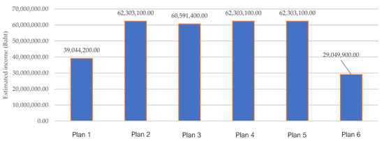
Figure 7.
Comparison of estimated income of the suitable agricultural areas for water utilization areas.
4.4. Managerial Implications
This study contributes to both the theoretical development of the knowledge and practical implication of the use of DSS for crop planning. For the theoretical development, it is clearly shown that the proposed of mathematical model and metaheuristics algorithm embedded in a DSS is a novel contribution to the knowledge pool. Meanwhile, in practice, the use case of DSS for crop planning proposed in this study is more suitable for tactical DSS which are for short to middle-term, seasonal economic decisions. The decision maker can use the DSS to aid his/her consideration in the planning for water distribution and crop planning in the following season. The DSS can provide the decision maker information regarding the economic benefit of each plan. However, DSS that account for economic scenarios ideally should also account for uncertainty risk. The proposed DSS currently lacks this feature. It is planned to be addressed as a future research direction.
5. Conclusions and Future Research Directions
This study proposed the decision support system (DDS) for crop planning. The optimization and scheduling model is formulated to determine the optimal cropping pattern and the water resource allocation in an irrigation area to maximize the net economic benefit and maximize crop area in the Huay Mae Tho reservoir case study. The constraints consisted of the constrictions of the area’s characteristics, water requirements, water availability, cropping area of each irrigation zones, and the cropping pattern alternatives. DDS provides the SA to solve the model. The results show that it can obtain the optimal solution the same as the exact solution obtained. Further analysis of the availability of crop pattern scenarios demonstrated that the current plan implemented in the Huay Mae Tho reservoir has the potential to be improved further.
Despite several promising results shown in the experiment, the analysis provided in this study consist of only several limiting factors such as the expected crop yield, crop price, land area availability, and water availability. We have not yet tackled many complicated considerations that might be available in the field. Therefore, future research direction may need to consider more factors that might appear in the area, such as the uncertainty of water availability, demand changes, and the risk of crop failures. Furthermore, the implementation of the SA algorithm in larger size instances might show the advantage of the algorithm even more. In addition, a combination of the exact solution approach and approximation approach is nowadays a trend in solving this type of problem.
Author Contributions
Conceptualization, P.J., P.N., M.F.N.M. and A.A.N.P.R.; methodology, P.J., P.N. and A.A.N.P.R.; software, A.A.N.P.R.; validation, P.J., J.D.G., M.F.N.M. and A.A.N.P.R.; formal analysis, P.J., M.F.N.M. and A.A.N.P.R.; resources, P.J.; data curation, P.J. and A.A.N.P.R.; writing—original draft preparation, P.J. and M.F.N.M.; writing—review and editing, P.J., M.F.N.M. and A.A.N.P.R.; visualization, P.J., M.F.N.M. and A.A.N.P.R.; supervision, P.J.; project administration, P.J. and A.A.N.P.R.; funding acquisition, P.J. and J.D.G. All authors have read and agreed to the published version of the manuscript.
Funding
This research was funded by Mapua University Directed Research for Innovation and Value Enhancement (DRIVE).
Institutional Review Board Statement
Not applicable.
Informed Consent Statement
Informed consent was obtained from all subjects involved in this study.
Data Availability Statement
The data that support the findings of this study are available from the corresponding author upon reasonable request.
Acknowledgments
This research was partially supported by the National Research Council of Thailand (NRCT). This support is gratefully acknowledged.
Conflicts of Interest
The authors declare no conflict of interest.
References
- Zecca, F. The Use of Internet of Things for the Sustainability of the Agricultural Sector: The Case of Climate Smart Agriculture. Int. J. Civ. Eng. Technol. 2019, 10, 494–501. [Google Scholar]
- Lampridi, M.G.; Sørensen, C.G.; Bochtis, D. Agricultural Sustainability: A Review of Concepts and Methods. Sustainability 2019, 11, 5120. [Google Scholar] [CrossRef]
- Haque, F.F.; Abdelgawad, A.; Yanambaka, V.P.; Yelamarthi, K. Crop Yield Prediction Using Deep Neural Network. In Proceedings of the 2020 IEEE 6th World Forum on Internet of Things (WF-IoT), New Orleans, LA, USA, 2–16 June 2020; pp. 1–4. [Google Scholar]
- Kouadio, L.; Deo, R.C.; Byrareddy, V.; Adamowski, J.F.; Mushtaq, S.; Phuong Nguyen, V. Artificial Intelligence Approach for the Prediction of Robusta Coffee Yield Using Soil Fertility Properties. Comput. Electron. Agric. 2018, 155, 324–338. [Google Scholar] [CrossRef]
- Pourmohammadali, B.; Hosseinifard, S.J.; Hassan Salehi, M.; Shirani, H.; Esfandiarpour Boroujeni, I. Effects of Soil Properties, Water Quality and Management Practices on Pistachio Yield in Rafsanjan Region, Southeast of Iran. Agric. Water Manag. 2019, 213, 894–902. [Google Scholar] [CrossRef]
- Arsenovic, M.; Karanovic, M.; Sladojevic, S.; Anderla, A.; Stefanovic, D. Solving Current Limitations of Deep Learning Based Approaches for Plant Disease Detection. Symmetry 2019, 11, 939. [Google Scholar] [CrossRef]
- Hernández, S.; López, J.L. Uncertainty Quantification for Plant Disease Detection Using Bayesian Deep Learning. Appl. Soft Comput. 2020, 96, 106597. [Google Scholar] [CrossRef]
- Darwish, A.; Ezzat, D.; Hassanien, A.E. An Optimized Model Based on Convolutional Neural Networks and Orthogonal Learning Particle Swarm Optimization Algorithm for Plant Diseases Diagnosis. Swarm Evol. Comput. 2020, 52, 100616. [Google Scholar] [CrossRef]
- Zhang, W.; Liu, H.; Wu, W.; Zhan, L.; Wei, J. Mapping Rice Paddy Based on Machine Learning with Sentinel-2 Multi-Temporal Data: Model Comparison and Transferability. Remote Sens. 2020, 12, 1620. [Google Scholar] [CrossRef]
- Nguyen Thanh Le, V.; Apopei, B.; Alameh, K. Effective Plant Discrimination Based on the Combination of Local Binary Pattern Operators and Multiclass Support Vector Machine Methods. Inf. Process. Agric. 2019, 6, 116–131. [Google Scholar] [CrossRef]
- Goldstein, A.; Fink, L.; Meitin, A.; Bohadana, S.; Lutenberg, O.; Ravid, G. Applying Machine Learning on Sensor Data for Irrigation Recommendations: Revealing the Agronomist’s Tacit Knowledge. Precis. Agric. 2018, 19, 421–444. [Google Scholar] [CrossRef]
- Gutiérrez, S.; Diago, M.P.; Fernández-Novales, J.; Tardaguila, J. Vineyard Water Status Assessment Using On-the-Go Thermal Imaging and Machine Learning. PLoS ONE 2018, 13, e0192037. [Google Scholar] [CrossRef] [PubMed]
- Taghizadeh-Mehrjardi, R.; Nabiollahi, K.; Rasoli, L.; Kerry, R.; Scholten, T. Land Suitability Assessment and Agricultural Production Sustainability Using Machine Learning Models. Agronomy 2020, 10, 573. [Google Scholar] [CrossRef]
- Ferrández-Pastor, F.J.; García-Chamizo, J.M.; Nieto-Hidalgo, M.; Mora-Pascual, J.; Mora-Martínez, J. Developing Ubiquitous Sensor Network Platform Using Internet of Things: Application in Precision Agriculture. Sensors 2016, 16, 1141. [Google Scholar] [CrossRef]
- Wolfert, S.; Ge, L.; Verdouw, C.; Bogaardt, M.J. Big Data in Smart Farming—A Review. Agric. Syst. 2017, 153, 69–80. [Google Scholar] [CrossRef]
- López-Riquelme, J.A.; Pavón-Pulido, N.; Navarro-Hellín, H.; Soto-Valles, F.; Torres-Sánchez, R. A Software Architecture Based on FIWARE Cloud for Precision Agriculture. Agric. Water Manag. 2017, 183, 123–135. [Google Scholar] [CrossRef]
- Udias, A.; Pastori, M.; Dondeynaz, C.; Carmona Moreno, C.; Ali, A.; Cattaneo, L.; Cano, J. A Decision Support Tool to Enhance Agricultural Growth in the Mékrou River Basin (West Africa). Comput. Electron. Agric. 2018, 154, 467–481. [Google Scholar] [CrossRef]
- Bazzani, G.M. An Integrated Decision Support System for Irrigation and Water Policy Design: DSIRR. Environ. Model. Softw. 2005, 20, 153–163. [Google Scholar] [CrossRef]
- Bonfante, A.; Monaco, E.; Manna, P.; De Mascellis, R.; Basile, A.; Buonanno, M.; Cantilena, G.; Esposito, A.; Tedeschi, A.; De Michele, C.; et al. LCIS DSS—An Irrigation Supporting System for Water Use Efficiency Improvement in Precision Agriculture: A Maize Case Study. Agric. Syst. 2019, 176, 102646. [Google Scholar] [CrossRef]
- Basso, B.; Cammarano, D.; Fiorentino, C.; Ritchie, J.T. Wheat Yield Response to Spatially Variable Nitrogen Fertilizer in Mediterranean Environment. Eur. J. Agron. 2013, 51, 65–70. [Google Scholar] [CrossRef]
- Li, F.Y.; Johnstone, P.R.; Pearson, A.; Fletcher, A.; Jamieson, P.D.; Brown, H.E.; Zyskowski, R.F. AmaizeN: A Decision Support System for Optimizing Nitrogen Management of Maize. NJAS Wageningen J. Life Sci. 2009, 57, 93–100. [Google Scholar] [CrossRef][Green Version]
- Nelson, R.A.; Holzworth, D.P.; Hammer, G.L.; Hayman, P.T. Infusing the Use of Seasonal Climate Forecasting into Crop Management Practice in North East Australia Using Discussion Support Software. Agric. Syst. 2002, 74, 393–414. [Google Scholar] [CrossRef]
- Han, E.; Ines, A.V.M.; Baethgen, W.E. Climate-Agriculture-Modeling and Decision Tool (CAMDT): A Software Framework for Climate Risk Management in Agriculture. Environ. Model. Softw. 2017, 95, 102–114. [Google Scholar] [CrossRef]
- Thorburn, P.J.; Jakku, E.; Webster, A.J.; Everingham, Y.L. Agricultural Decision Support Systems Facilitating Co-Learning: A Case Study on Environmental Impacts of Sugarcane Production. Int. J. Agric. Sustain. 2011, 9, 322–333. [Google Scholar] [CrossRef]
- Soltani, A.; Stoorvogel, J.J.; Veldkamp, A. Model Suitability to Assess Regional Potato Yield Patterns in Northern Ecuador. Eur. J. Agron. 2013, 48, 101–108. [Google Scholar] [CrossRef]
- National Economic and Social Development Council NESDC ECONOMIC REPORT Thai Economic Performance in Q1 and Outlook for 2019 Economic Outlook. 2019, 2019, 1–32. Available online: https://www.nesdc.go.th/nesdb_en/ewt_dl_link.php?nid=4379&filename=Macroeconomic_Planning (accessed on 20 October 2021).
- Ministry of Commerce. Major Exports of Thailand in Accordance with the Structure of World Exports. Available online: http://tradereport.moc.go.th/Report/ReportEng.aspx?Report=MenucomRecode&Option=5&Lang=Eng (accessed on 12 October 2021).
- Food and Agricultural Organization of United Nations. FAOSTAT: Thailand. Available online: http://www.fao.org/faostat/en/#country/216 (accessed on 10 October 2021).
- United Nations Thailand. Thai Agricultural Sector: From Problems to Solutions. Available online: https://thailand.un.org/en/103307-thai-agricultural-sector-problems-solutions (accessed on 10 October 2021).
- Climate-data.org. Climate Tak (Thailand). Available online: https://en.climate-data.org/asia/thailand/tak-province/tak-2939/#climate-graph (accessed on 10 October 2022).
- National Statistical Office. Agricultural Census; National Statistical Office: Bangkok, Thailand, 2013.
- Attavanich, W.; Chantarat, S.; Chenphuengpawn, J.; Mahasuweerachai, P.; Thampanishvong, K. Farms, Farmers and Farming: A Perspective through Data and Behavioral Insights. 2019. Available online: https://www.pier.or.th/files/dp/pier_dp_122.pdf (accessed on 21 January 2022).
- Allen, R.G.; Pereira, L.S.; Raes, D.; Smith, M. Crop Evapotranspiration—Guidelines for Computing Crop Water Requirements—FAO Irrigation and Drainage Paper 56; Food and Agriculture Organization of the United Nations: Rome, Italy, 1998.
- McNaughton, K.G.; Jarvis, P.G. Using the Penman-Monteith Equation Predictively. In Evapotranspiration from Plant Communities; Sharma, M.L., Ed.; Elsevier: Amsterdam, The Netherlands, 1984; Volume 13, pp. 263–278. ISBN 0166-2287. [Google Scholar]
- Thai Meteorological Department. Climatological Data for The Period 1981–2010. Available online: http://www.climate.tmd.go.th/content/article/75 (accessed on 8 October 2021).
- Ministry of Agricultural Economics Thailand. Tak City Agriculture Area in 2020. Available online: http://mis-app.oae.go.th/area/%E0%B8%A5%E0%B8%B8%E0%B9%88%E0%B8%A1%E0%B9%81%E0%B8%A1%E0%B9%88%E0%B8%99%E0%B9%89%E0%B8%B3/%E0%B9%81%E0%B8%A1%E0%B9%88%E0%B8%99%E0%B9%89%E0%B8%B3%E0%B8%A2%E0%B8%A1/%E0%B8%95%E0%B8%B2%E0%B8%81 (accessed on 20 July 2021).
- Maghfiroh, M.F.N.; Hanaoka, S. Multi-Period Evacuation Shelter Selection Considering Dynamic Hazards Assessment. Indones. J. Comput. Eng. Des. 2019, 1, 64. [Google Scholar] [CrossRef]
- Lukovac, V.; Pamučar, D.; Popović, M.; Đorović, B. Portfolio Model for Analyzing Human Resources: An Approach Based on Neuro-Fuzzy Modeling and the Simulated Annealing Algorithm. Expert Syst. Appl. 2017, 90, 318–331. [Google Scholar] [CrossRef]
- Haznedar, B.; Kalinli, A. Training ANFIS Structure Using Simulated Annealing Algorithm for Dynamic Systems Identification. Neurocomputing 2018, 302, 66–74. [Google Scholar] [CrossRef]
- Yu, V.F.; Jewpanya, P.; Redi, A.A.N.P.; Tsao, Y.-C. Adaptive Neighborhood Simulated Annealing for the Heterogeneous Fleet Vehicle Routing Problem with Multiple Cross-Docks. Comput. Oper. Res. 2021, 129, 105205. [Google Scholar] [CrossRef]
- Yu, V.F.; Jewpanya, P.; Redi, A.A.N.P. Open Vehicle Routing Problem with Cross-Docking. Comput. Ind. Eng. 2016, 94, 6–17. [Google Scholar] [CrossRef]
- Redi, A.A.N.P.; Jewpanya, P.; Kurniawan, A.C.; Persada, S.F.; Nadlifatin, R.; Dewi, O.A. A Simulated Annealing Algorithm for Solving Two-Echelon Vehicle Routing Problem with Locker Facilities. Algorithms 2020, 13, 218. [Google Scholar] [CrossRef]
- Reinaldi, M.; Redi, A.A.; Prakoso, D.F.; Widodo, A.W.; Wibisono, M.R.; Supranartha, A.; Liperda, R.I.; Nadlifatin, R.; Prasetyo, Y.T.; Sakti, S. Solving the Two Echelon Vehicle Routing Problem Using Simulated Annealing Algorithm Considering Drop Box Facilities and Emission Cost: A Case Study of Reverse Logistics Application in Indonesia. Algorithms 2021, 14, 259. [Google Scholar] [CrossRef]


Publisher’s Note: MDPI stays neutral with regard to jurisdictional claims in published maps and institutional affiliations. |
© 2022 by the authors. Licensee MDPI, Basel, Switzerland. This article is an open access article distributed under the terms and conditions of the Creative Commons Attribution (CC BY) license (https://creativecommons.org/licenses/by/4.0/).