Article

Speed Tracking Control of High-Speed Train Based on Particle Swarm Optimization and Adaptive Linear Active Disturbance Rejection Control

College of Automation and Electronic Engineering, Qingdao University of Science and Technology, Qingdao 266061, China
*
Author to whom correspondence should be addressed.
Appl. Sci. 2022, 12(20), 10558; https://doi.org/10.3390/app122010558
Submission received: 19 September 2022 / Revised: 14 October 2022 / Accepted: 17 October 2022 / Published: 19 October 2022

Abstract

:
This paper proposes a control scheme combining improved particle swarm optimization (IPSO) and adaptive linear active disturbance rejection control (ALADRC) to solve the high-speed train (HST) speed tracking control problem. Firstly, in order to meet the actual operation of a HST, a multi-mass point dynamic model with time-varying coefficients was established. Secondly, linear active disturbance rejection control (LADRC) was proposed to control the speed of the HST, and the anti-disturbance ability of the system was improved by estimating and compensating for the total disturbance suffered by the carriage during the operation of the HST. Meanwhile, to solve the problem of difficult parameter tuning of the LADRC, IPSO was introduced to optimize the parameters. Thirdly, the adaptive control (APC) was introduced to compensate for the observation error caused by the bandwidth limitation of the linear state expansion observer in LADRC and the tracking error caused by an unknown disturbance during the train’s operation. Additionally, the Lyapunov theory was used to prove the stability of the system. Finally, the simulation results showed that the designed control scheme is more effective in solving the problem of HST speed tracking.

1. Introduction

The high-speed train has become the most popular travel mode in the past decade, because of its fast, economic, stable, and safe characteristics [1]. In order to meet growing travel demands, many countries have been vigorously developing high-speed railways [2,3,4]. At the same time, the HST automatic driving strategy also needs continuous improvement and perfection. As one of the key subsystems of the automatic train control system, the automatic train operation (ATO) system is responsible for controlling the traction and braking of the HST, and its most important function is to control the speed of the HST, which is the basis for achieving automatic HST operation and operational safety [5,6]. Thus, it is important to understand how to use the ATO system to realize HST speed tracking in a complex environment [7].
Over the past few years, the problem of ATO has attracted great attention from researchers in theoretical and engineering fields. This has also led to the discovery of many efficient algorithms [8]. In 1960, PID control was first applied to the ATO system. Although the application of PID has improved the tracking accuracy, its anti-disturbance ability and comfort still cannot meet the requirements [9]. In [10], an adaptive fuzzy sliding mode controller was designed to realize high-precision train parking by processing nonlinear switching signals. In [11], to improve the anti-disturbance ability of HST during cruise, an improved sliding mode controller was proposed to reduce the chattering caused by controller switching. In [12], according to two different signal transmission modes between carriages, an adaptive control law was designed to realize high-precision speed tracking of the whole train process. In addition, many control strategies such as fuzzy control, predictive control, and some optimization algorithms have been applied to the design of ATO systems [13,14,15,16]. Compared with the PID controller, the above control strategies have a better control effect. However, the design of most control strategies is cumbersome, and it is necessary to establish an accurate HST mathematical model [17]. However, the interference of HSTs during operation is complex and unknown, and the HST itself has nonlinear and strong coupling characteristics. Thus, it is impractical to establish an accurate mathematical model of the HST. Therefore, it is necessary to design a speed tracking controller which does not depend on an accurate HST model and has strong anti-disturbance ability and high accuracy.
Based on the idea of classical PID error feedback processing, a nonlinear active disturbance rejection control (ADRC) was proposed in [18]. However, ADRC has too many parameters that need to be set, which is not conducive to the application of practical engineering. Therefore, the nonlinear link in ADRC was linearized, and the linear active disturbance rejection control (LADRC) was proposed [19]. The LADRC mainly includes the linear tracking differentiator (LTD), linear extended state observation (LESO), and PD controller [20]. LESO can observe and compensate for the total disturbance of the system in real-time, which makes LADRC have a good anti-disturbance performance. This also greatly promotes the application of LADRC in practical engineering [21]. In [22], in order to solve the stability and fast response of the gas flowmeter in the testing process, a decoupling controller of gas flow facility was proposed based on LADRC. The overall influence of the two channels of internal uncertainty and external disturbance in the system was observed as the total disturbance through LESO. This can decouple the pressure–flow coupling system into two single-input and single-output systems. The simulation results showed that LADRC has stronger anti-disturbance performance and better decoupling effect compared with PID. In [23,24], in order to improve the dynamic capability of the distribution network in the case of various grid defects, an improved LADRC controller was used to improve the control performance by compensating for the LESO observation disturbance error. The results showed that the improved LADRC can better reduce the voltage fluctuation caused by the system and improve the power grid efficiency. In [25], LADRC was proposed to solve the problem of accurately tracking the planned trajectory of Delta high-speed parallel robots. The internal coupling and disturbance of the robot were observed and compensated by the state observer to solve the problem of strong couplings in the system. Finally, compared with the PID control, the experimental results showed that the Delta high-speed robot with LADRC had better response speed, tracking accuracy, and stronger robustness. Meanwhile, LADRC has also been widely used in other fields [26,27,28,29]. Although LADRC has many advantages, it still needs to readjust its parameters for different systems. Moreover, due to the bandwidth limitation of LESO, some disturbance estimation errors may be caused, resulting in low control accuracy [30]. Therefore, finding a simple and efficient LADRC parameter tuning method and real-time compensation for the observation disturbance error of LESO can greatly improve the control performance of LADRC.
Therefore, in order to ensure that HSTs can still track the ideal speed signal stably and accurately under the influence of various additional resistances and change in coefficients, the main contributions of this paper are summarized as follows:
(1)
In this paper, a multi-mass point HST model with time-varying coefficients is selected as the controlled object, which is more in line with the actual operation;
(2)
A control scheme combining IPSO and ALADRC is proposed to solve the problem of HST speed tracking. As the main controller, LADRC can estimate and compensate for the total disturbance of the system in real-time. This enables each carriage with the traction unit to be controlled independently by LADRC to ensure the stability of HSTs during operation;
(3)
In order to solve the problem of parameter settings in LADRC, IPSO is proposed to optimize the four key parameters k p , k d , w , and b in LADRC with the goal of minimizing the HST speed tracking error. By this method, LADRC can quickly and accurately obtain better parameter values under the ideal conditions of known route, which greatly simplifies the parameter setting process;
(4)
In order to adapt LADRC to the complex and changeable operating environment and to solve the problem of LESO, slight observation errors may be caused due to bandwidth limitations. Thus, APC is introduced. The combination of LADRC and APC can effectively improve the control performance when LADRC encounters unknown disturbances. The stability of the whole system can also be proved by the Lyapunov stability theory. Finally, by comparing with LADRC, it is verified that the designed control has more advantages in HST speed tracking.
The rest of the paper is organized as follows: a HST multi-mass point model is given in Section 2; the design of the control scheme and the verification of the stability of the system using Lyapunov’s stability theory are given in Section 3; the design of the HST operation speed curve and the simulation results of two control schemes are given in Section 4; and the conclusion is given in the last section.

2. Dynamic Model of a High-Speed Train

The HST is subject to a variety of forces during operation. Each carriage is subject to traction and braking forces u from the traction unit, basic operating resistance f a , additional resistance f b , and interaction forces f d between the carriages. The basic running resistance f a is the resistance that the HST must be subjected to during operation, including the friction between the HST internal components, rolling resistance, and air resistance. Its calculation equation satisfies the Davis equation [31]:
f a ( v ) = c o + c v v + c a v 2
where c o , c v , and c a are Davis coefficients, and their values are generally determined by empirical constants. c o is the rolling mechanical resistance coefficient independent of train speed, c v is the rolling friction resistance coefficient, and c a is the air resistance coefficient.
The additional running resistance f b represents the running resistance generated when the HST passes through ramps, curves, and tunnels. Its calculation equation is as follows:
f 1 = m g θ f 2 = m g ( 600 / R ) f 3 = m g ( 0.00013 L )
where g = 9.8   m / s 2 is the acceleration of gravity, m is the mass of a single carriage, f 1 is the ramp additional resistance, θ is the angle between the track and the horizontal road surface, f 2 is the curve additional resistance, R is the curve radius, f 3 is the tunnel additional resistance, and L is the tunnel length. The additional resistance during HST operation can be expressed as f b = f 1 + f 2 + f 3 .
The HST is a multi-body system consisting of multiple carriages connected by hooks. f d is the interaction force between carriages during operation. Each carriage is subjected to the coupling force from other carriages, which can be expressed by an “elastic-damping” structure [32] as:
f d i ( i + 1 ) = k ( x i x i + 1 ) + d ( v i v i + 1 )
where f d i ( i + 1 ) is the interaction force between carriage i and carriage i + 1 , k and d are the elastic coupling coefficient and damping coupling coefficient of the hook, respectively, and x i and v i are the displacement and speed of the carriage i , respectively.
In summary, the force analysis of each carriage according to Newton’s laws of motion can describe the HST multi-mass model as:
m 1 v ˙ 1 = u 1 f a 1 f d 12 f b 1 m i v ˙ i = u i f a i f d i ( i + 1 ) + f d ( i 1 ) i f b i     ( i = 2 , 3 , n 1 ) m n v ˙ n = u n f a n + f d ( n 1 ) n f b n x ˙ i = v i ,   ( i = 1 , 2 , , n )
where n is the number of carriages and u i stands for traction or braking force output.
Remark 1.
In a general simulation [33], the coefficients c o , c v , and c a of the Davis equation and the mass m of a single carriage are generally fixed values determined by empirical constants. However, the value of these part coefficients will not be constant due to the change of a HST’s running line environment, the difference of track adhesion, the consumption of the train itself, and the movement of carriage personnel. Therefore, the uncertain time-varying coefficients c o , c v , c a , and m are adopted in this paper, which is more consistent with the actual situation.

3. Design of the Control Scheme

3.1. Design of the High-Speed Train Speed Control System

The four carriages of a HST are selected as the research objects in this paper, and the first and the fourth carriages have traction units. Figure 1 shows the structure of the control scheme. In order to solve the speed tracking control problem of the high-speed train, a control scheme combining IPSO and ALADRC is proposed. Since the two LADRC work in different carriages during HST operation, the two LADRC parameters may be inconsistent due to the interaction between carriages. In known lines, the parameters of two LADRC are optimized and adjusted by the IPSO algorithm according to the principle of minimum tracking error. This method can ensure that two LADRC have better parameters at the same time. In addition, APC is introduced to ensure that LADRC still has good control performance under unknown disturbance. This makes LADRC compensate for the observation error caused by the bandwidth limitation of LESO according to the HST tracking error. Meanwhile, the parameters of the PD controller can be adjusted to eliminate the speed fluctuation caused by disturbance. This can also effectively improve the control accuracy and anti-disturbance performance of LADRC.
Remark 2.
In this paper, LESO can observe each state variable of the HST system and the total system disturbance according to the input and output data. Due to the discretization of the observer, the bandwidth value of LESO cannot exceed the sampling period of the system, as it will lead to the divergence of the LESO observation [30]. If the bandwidth value is minimal, it will lead to low LESO observation accuracy. APC is introduced to compensate for the observation error caused by bandwidth selection to improve the control accuracy and dynamic performance of LADRC. This method will make LADRC more adaptable and extensive.

3.2. Design of Improved Particle Swarm Optimization

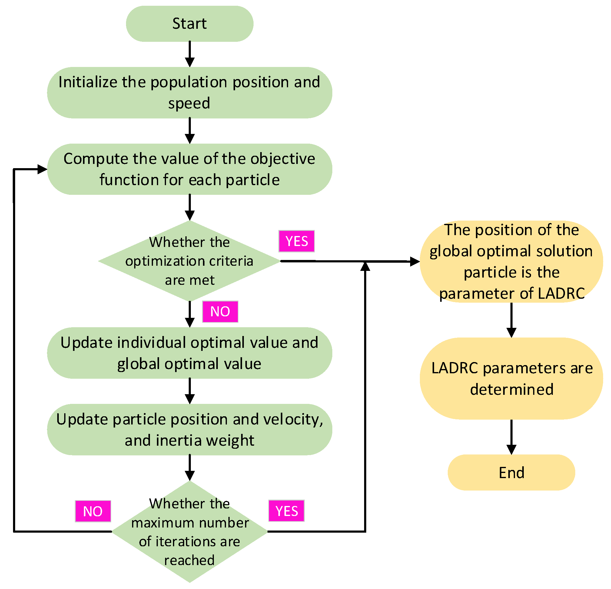
Particle swarm optimization (PSO) is widely used to solve optimization problems. It originated from research on the predation behavior of birds, and its idea is to find the optimal solution through cooperation and information sharing between individuals in the group [34]. Defining the particle search dimension is D , the number of particles in the population is N , and the number of iterations is M . During the search, the position of the particle n at the m - t h iteration is denoted as x n m = x n 1 m , x n 2 m x n D m and the velocity is denoted as v n m = v n 1 m , v n 2 m v n D m . During each iteration, the function value of the current position of each particle will be calculated according to the objective function, and the individual optimal solution and the global optimal solution will be updated in real-time. In the next iteration, each particle will update its velocity and position according to the individual and global optimal solutions. Meanwhile, the position interval [ x min ,   x max ] and velocity interval [ v min ,   v max ] of the particle are set to optimize the particle within the specified range. In this paper, the purpose of IPSO optimization is to ensure the minimum speed tracking error of all carriages by adjusting the parameters of two LADRC. The optimization process is shown in Figure 2.
During optimization, the position and velocity of each particle are updated according to the following equation:
v n m + 1 = w 0 v n m + c 1 r a n d 1 ( p b e s t n x n m ) + c 2 r a n d 2 ( g b e s t m x n m ) x n m + 1 = x n m + v n m + 1
where p b e s t n is the position of the individual optimal of particle n , and g b e s t m is the position of the global optimal of m - t h iteration. c 1 and c 2 are the learning factors to regulate the maximum step size of learning. r a n d 1 and r a n d 2 are the random numbers to increase the randomness of the search, and their range is 0   ,   1 , whilst w 0 is the inertia weight.
From (5), the value of w 0 affects the velocity of particle movement. When w 0 is large, it is beneficial to the global search of the population, but it will lead to the low accuracy of the local search in the later stage. When w 0 is small, it is beneficial to improve the accuracy of the local optimization of the population, but it may cause the population to fall into the local optimal solution. Therefore, the inertia weight with linear decline is selected, and its updating equation is as follows:
w 0 = w max m w max w min / M
where w max is the maximum inertia weight and w min is the minimum inertia weight. Since the beginning of the search, w 0 decreases linearly from w max to w min in order to ensure the global search and local search ability of the population.
In this paper, the integral of the absolute value of error criterion (IAE) is adopted as the objective function of IPSO, and the calculation equation is as follows:
J I A E = i = 1 4   0 T     v d v i       d t
where i is the number of the carriage and T is the total operation time of the HST. The optimization objective of IPSO is to ensure that the value of the objective function is as small as possible.

3.3. Design of Adaptive Linear Active Disturbance Rejection Control

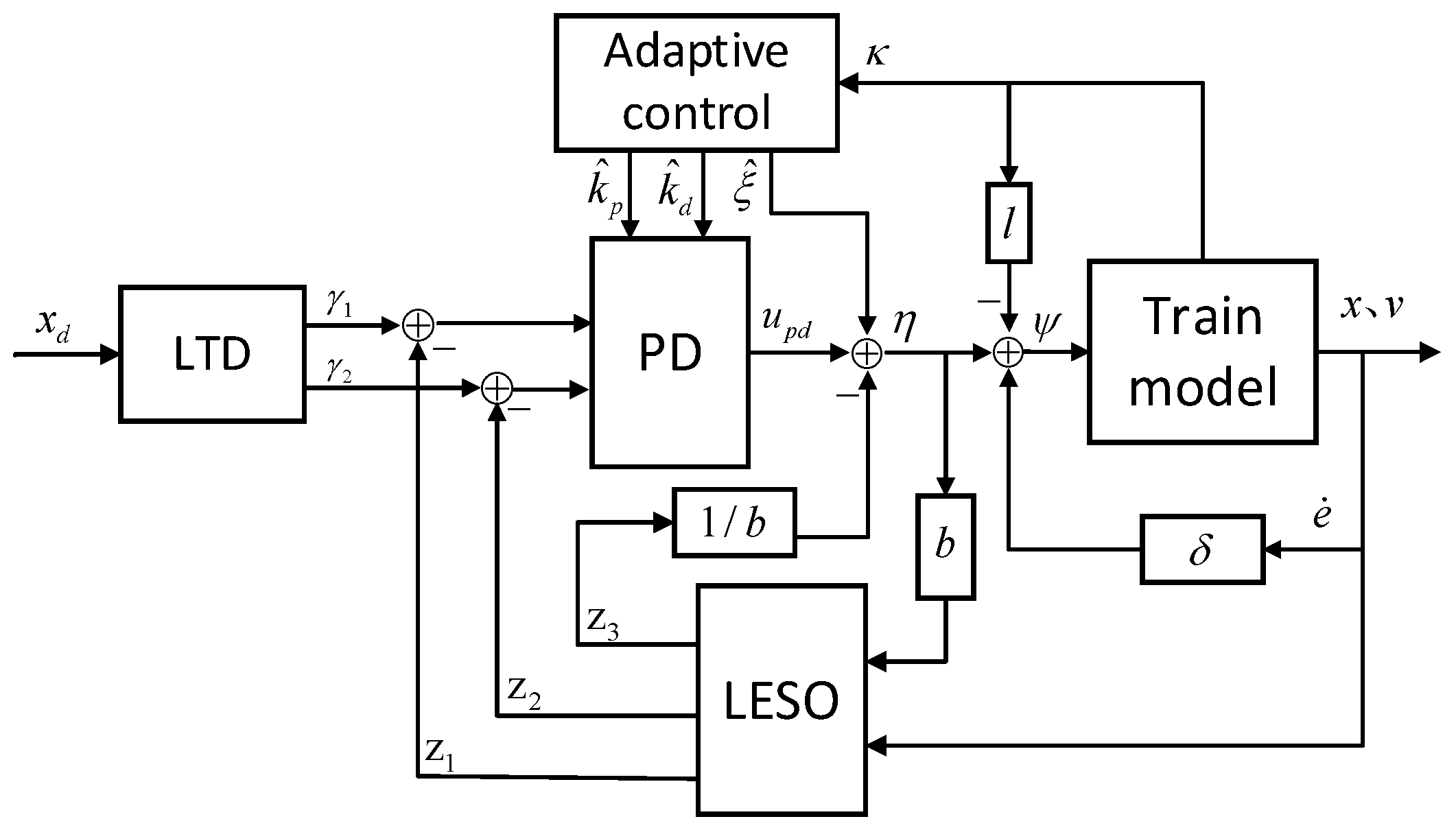
The structure of the ALADRC is shown in Figure 3. LADRC mainly consists of three parts: LTD, LESO, and PD controller. On the basis of IPSO parameter adjustment, APC can adjust k p and k d in the PD controller in real-time and compensate the observation error of LESO through the tracking error of the HST at the same time.
LTD is to arrange the transition process for the system. Its function is to make the input signal and its differential signal output smooth, to ensure the system can realize fast tracking and reduce overshooting. The design of LTD for carriage i draws on [35]:
γ ˙ 1 i = γ 2 γ ˙ 2 i = 1.76 α γ 2 i α 2 ( γ 1 i x d )
where α is an adjustable parameter to ensure that an appropriate transition process is arranged, whilst γ 1 i and γ 2 i are the signals that arrange the transition process for the ideal displacement signal x d of carriage i .
Due to the observation ability of LESO, LADRC has a natural decoupling function, which makes it possible to design a separate control law for a carriage with traction unit. According to (4), the dynamic model of the carriage i can be transformed into:
χ ˙ 1 i = χ 2 i χ ˙ 2 i = G i ( t ) + f i ( t ) + d i u i ( t ) y i = χ 1 i
where, χ 1 i and χ 2 i are measurable state variables, representing the position and speed of carriage i , respectively. G i ( t ) is an unknown nonlinear function of the system and the interaction force between the carriages, f i ( t ) is the basic running resistance, the additional running resistance and the disturbance caused by the time-varying HST coefficients. d i is partially known and the known part is denoted as d 0 i .
The sum of the internal disturbance and external disturbance is defined as the total disturbance F i = G i ( t ) + f i ( t ) + ( d i d 0 i ) u i ( t ) . Rewrite (9) as follows:
χ ˙ 1 i = χ 2 i χ ˙ 2 i = G i ( t ) + f i ( t ) + ( d i d 0 i ) u i ( t ) + d 0 i u i ( t ) = d 0 i u i ( t ) + F i   y i = χ 1 i
Add an extended state variable χ 3 i = F i to represent the disturbance of the system. Thus, χ i = [ χ 1 i   χ 2 i   χ 3 i ] T is the extended state including the disturbance. Equation (10) can be translated into a state extension space description as:
χ ˙ i = Q χ i + M i u i + N F ˙ i y i = U χ i
where Q = 0 1 0 0 0 1 0 0 0 , M i = 0 d 0 i 0 , N = 0 0 1 and U = [ 1   0   0 ] .
According to (11), the design of LESO for carriage i is as follows:
z ˙ i = Q z i + M i u i + P ( y i y ^ i ) y ^ i = U z i
where z i = [ z 1 i   z 2 i   z 3 i ] T is the state vector of the observer, which is used to observe the state of system χ i = [ χ 1 i   χ 2 i   χ 3 i ] T . P = [ P 1   P 2   P 3 ] T is the observation gain matrix of LESO. The observation gain is parameterized by placing all eigenvalues at the observation bandwidth and the observer gain is obtained from its characteristic equation:
λ ( s ) = ( s + ω ) 3 = s 3 + P 1 s 2 + P 2 s + P 3
the observer gain can be obtained as P = [ 3 ω   3 ω 2   ω 3 ] T , where ω is the bandwidth of LESO.
The control law of LADRC for carriage i is defined as η i :
η i = u p d i z 3 i / b + ξ i
where u p d i = k p i ( s 1 i z 1 i ) + k d i ( s 2 i z 2 i ) is the control signal output of the PD controller in LADRC for carriage i , and k p i and k d i are the gain parameters. ξ i is the compensation signal of LESO observation error, whilst z 3 i / b is the compensation signal of total disturbance.
According to the HST dynamic model (4), the dynamic model of a single carriage i is as follows:
m i x ¨ i = u i c o i + c v i x ˙ i + c a i x ˙ i 2 f d i ( i + 1 ) + f d ( i 1 ) i f b i
Define the displacement and speed tracking error of carriage i as e i = x i x d and e ˙ i = v i v d , where x d and v d are the given desired displacement and speed signal, respectively. The adaptive value of the LESO observation error is defined as ξ ^ i , and the adaptive values of parameters k p i and k d i in the PD controller are defined as k ^ p i and k ^ d i , respectively. The adaptive estimation errors are ξ ˜ i = ξ ^ i ξ i , k ˜ p i = k ^ p i k p i and k ˜ d i = k ^ d i k d i , respectively.
Define a tracking error of carriage i as follows:
κ i t = e ˙ i + ρ e i ,     i = 1 , 2 , 3 , 4
to make sure that when e i 0 and e ˙ i 0 , then the ζ i 0 , and ρ is the appropriate constant selected.
Assumption 1. 
The given desired signal x d ( t ) and v d ( t ) is smooth and bounded, hence x d ( t ) X d and V d ( t ) V d , where X d and V d are known constants.
Taking the differential of κ i :
κ ˙ i = e ¨ i + ρ e ˙ i = x ¨ i x ¨ d + ρ x ˙ i x ˙ d
by introducing (15) into the above equation, it can be obtained:
m i κ ˙ i + x ¨ d ρ x ˙ i x ˙ d = u i c o i c v i x ˙ i c a i x ˙ i 2 f d i ( i + 1 ) + f d ( i 1 ) i f b i
then
m i κ ˙ i = u i c o i c v i x ˙ i c a i x ˙ i 2 m i x ¨ d ρ e ˙ i f d i ( i + 1 ) + f d ( i 1 ) i f b i
The design of carriage i control law ψ i is as follows:
ψ i = η i l κ i + m i x ¨ d ρ e ˙ i + ξ ^ i
where l is an arbitrary positive parameter and the coefficient δ in Figure 3 is m i ( x ¨ d ρ e ˙ i ) in the above equation. Bring the control law of LADRC (14) into above equation:
ψ i = u p d i z 3 i / b l κ i + m i x ¨ d ρ e ˙ i + ξ ^ i
Bring the control law (21) into (19):
m i κ ˙ i = u p d i l κ i + c o i + c v i x ˙ i + c a i x ˙ i 2 z 3 i / b f d i ( i + 1 ) + f d ( i 1 ) i f b i + ξ ^ i
due to the observation disturbance ability of LESO, the above equation can be further simplified as:
m i κ ˙ i = l κ i + k ^ p i γ 1 i z 1 i + k ^ d i γ 2 i z 2 i + ξ ˜ i

3.4. System Stability Analysis

Theorem 1.
Combined with the system (15), it is assumed that the following adaptive laws designed for carriage  i are effective:
ξ ^ ˙ i = φ ξ κ i k ^ ˙ p i = φ p [ κ i k ^ p i ( γ 1 i z 1 i ) ] / k ˜ p i k ^ ˙ d i = φ d [ κ i k ^ d i ( γ 2 i z 2 i ) ] / k ˜ d i
where φ ξ , φ p , and φ d are reasonable positive parameters.
Remark 3.
In order to adjust k p i and k d i on the basis of IPSO parameter setting, an initial value k p 0 i and k d 0 i can be set according to the parameters obtained by IPSO. This can also avoid k p i and k d i being 0, and the adaptive law can be rewritten:
k ^ p i = 0 T φ p [ κ i k ^ p i ( γ 1 i z 1 i ) ] / k ˜ p i   d t + k p 0 i k ^ d i = 0 T φ d [ κ i k ^ d i ( γ 2 i z 2 i ) ] / k ˜ d i   d t + k d 0 i
Theorem 2.
Considering the HST system (4), under Assumption 1, the designed control laws (14), (20), and adaptive laws (24), then it is proved that all signals of the system are bounded, and the system is in uniform stability.
Proof of Theorems 1 and 2. 
Referring to [36], a positive definite Lyapunov function is defined as follows:
V ( t ) = i = 1 n 1 2 m i κ i 2 + 1 2 φ ξ ξ ˜ i 2 + 1 2 φ p k ˜ p i 2 + 1 2 φ d k ˜ d i 2
Differentiate of the above equation for time:
V ˙ ( t ) = i = 1 n m i κ ˙ i κ i + 1 φ ξ ξ ˜ i ξ ˜ ˙ i + 1 φ p k ˜ p i k ˜ ˙ p i + 1 φ d k ˜ d i k ˜ ˙ d i
bring (23) into the above equation to obtain:
V ˙ ( t ) = i = 1 n κ i l κ i + k ^ p i γ 1 i z 1 i + k ^ d i γ 2 i z 2 i + ξ ˜ i + 1 φ ξ ξ ˜ i ξ ˜ ˙ i + 1 φ p k ˜ p i k ˜ ˙ p i + 1 φ d k ˜ d i k ˜ ˙ d i         = i = 1 n l κ i 2 + κ i k ^ p i γ 1 i z 1 i + k ^ d i γ 2 i z 2 i + ξ ˜ + 1 φ ξ ξ ˜ i ξ ^ ˙ i + 1 φ p k ˜ p i k ^ ˙ p i + 1 φ d k ˜ d i k ^ ˙ d i
bring the adaptive laws (24) into the above equation to obtain:
V ˙ ( t ) = i = 1 n l κ i 2 + κ i k ^ p i γ 1 i z 1 i k ˜ p i φ p φ p κ i k ^ p i γ 1 i z 1 i / k ˜ p i + κ i k ^ d i γ 2 i z 2 i k ˜ d i φ d φ d κ i k ^ d i γ 2 i z 2 i / k ˜ d i     + κ i ξ ˜ ξ ˜ i φ ξ φ ξ κ i
simplify the above equation:
V ˙ ( t ) = i = 1 n l κ i 2 0
From V ˙ ( t ) 0 and V ( t ) 0 , according to the Lyapunov stability theory, it can be proved that the system is in uniform stability. Meanwhile, all signals in the above equations are bounded, including tracking error κ ( t ) and its differential κ ˙ ( t ) . The proof is completed. □
Theorem 3.
If  κ ( t ) is a continuous function and satisfies the formula:
lim t 0 t   κ ( t )     d t = 0
then, it can be proved that the whole system is in uniform asymptotic stability.
Proof of Theorem 3:
Inference of Barbalat’s theorem: If κ ( t ) and κ ˙ ( t ) are bounded and κ ( t ) is square integrable, then:
lim t   κ ( t ) = 0
Due to V ( t ) being a monotonically decreasing function with upper and lower bounds, it can be obtained:
0 κ 2 ( t )   d t = V 0 V / l <
then, κ ( t ) is square integrable. And since κ ( t ) and κ ˙ ( t ) are bounded, κ ( t ) satisfies the inference of Barbalat’s theorem. Therefore, when t , it can obtain κ 0 and V ˙ < 0 , proving that the whole system is in uniform asymptotic stability. The proof is completed. □

4. Simulation Results and Analysis

The simulation results in this paper were obtained in MATLAB. The parameters used in the simulation are given in each part of the experiment.

4.1. System Stability Analysis

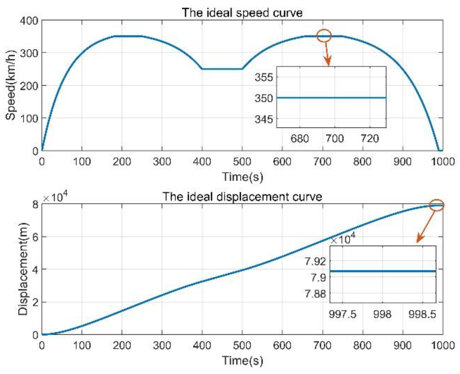
It is assumed that the HST operation route passes “start and traction–cruise–brake–cruise–traction–cruise–brake and stop”. The total operation time of HST is 1000   s , the total operation distance is 79 , 074   m , and the maximum operation speed is 350   km / h . The ideal speed and displacement curve is shown in Figure 4.
The HST will be affected by additional resistance during operation. It is assumed that the conditions of curves, ramps, and tunnels in the operation route are shown in Table 1.

4.2. Controller Parameter Optimization

This part is used to verify the feasibility of IPSO to optimize and adjust the parameters of LADRC in HSTs. IPSO needs to optimize the parameters k p , k d , w , and b of LADRC for the first and fourth carriages according to the objective function of (7) to simplify the parameter setting process. The parameters of each carriage are shown in Table 2. IPSO parameters are set as follows: c 1 = c 2 = 1 , N = 150 , M = 50 , D = 8 , w max = 1.2 , and w min = 0.6 .
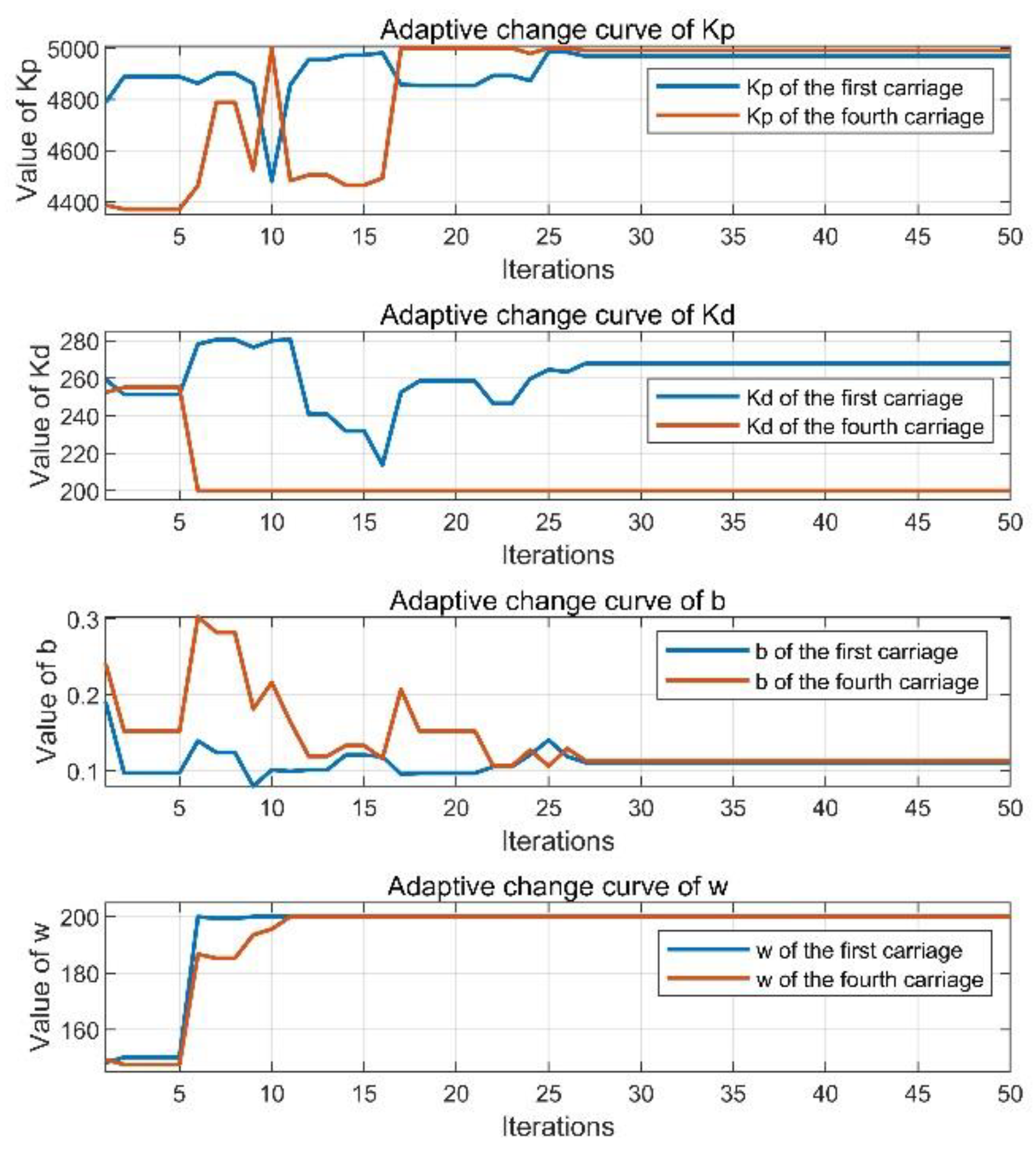
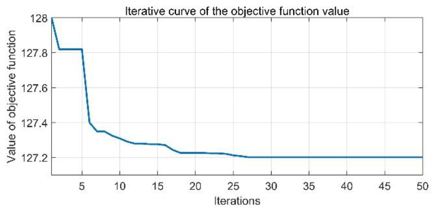
The change curve of LADRC parameters optimized by IPSO is shown in Figure 5, and the change curve of the IPSO objective function value is shown in Figure 6. From Figure 5, it can be seen that the parameter w is the fastest to find the optimal solution in the IPSO search process, and the parameter w for carriage 1 and carriage 4 are w 1 = 200 and w 4 = 200 , respectively. However, the parameters k p , k d , and b change many times, and finally the optimal solution was found in the 27th iteration. Their values are k p 1 = 4969 , k p 4 = 4991 , k d 1 = 268 , k d 4 = 200 , b 1 = 0.111 , and b 4 = 0.113 . As can be seen from Figure 6, the objective function value keeps shrinking in the IPSO optimization process, finally reaches the minimum value in the 27th iteration, and tends to be stable. It shows that the parameters of LADRC obtained at this time are optimal.

4.3. High-Speed Train Tracking Control

Example 1.
This part is used to verify the control performance of ALADRC when the HST has no coefficient time-varying during operation.The HST with ALADRC and LADRC operates in the same environment, and the control performance of the two controllers is reflected through the tracking of the ideal speed by the HST. ALADRC and LADRC have the same initial parameters, and their parameters come from the values obtained by IPSO optimization in Section B, as shown in Table 3. Other parameters are set as follows: φ ξ = φ p = φ d = 1 , α = 50 , and ρ = 0.5 .
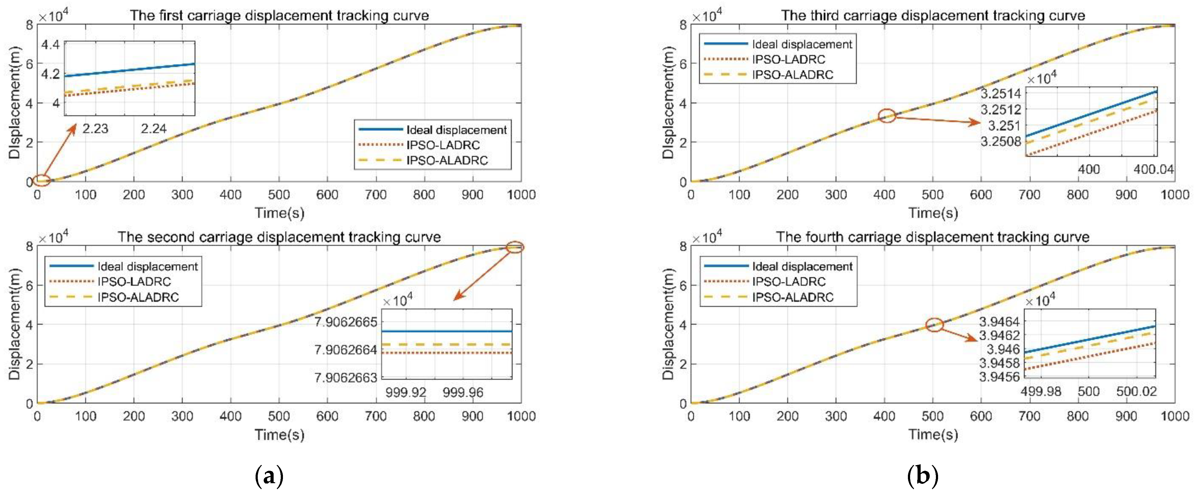
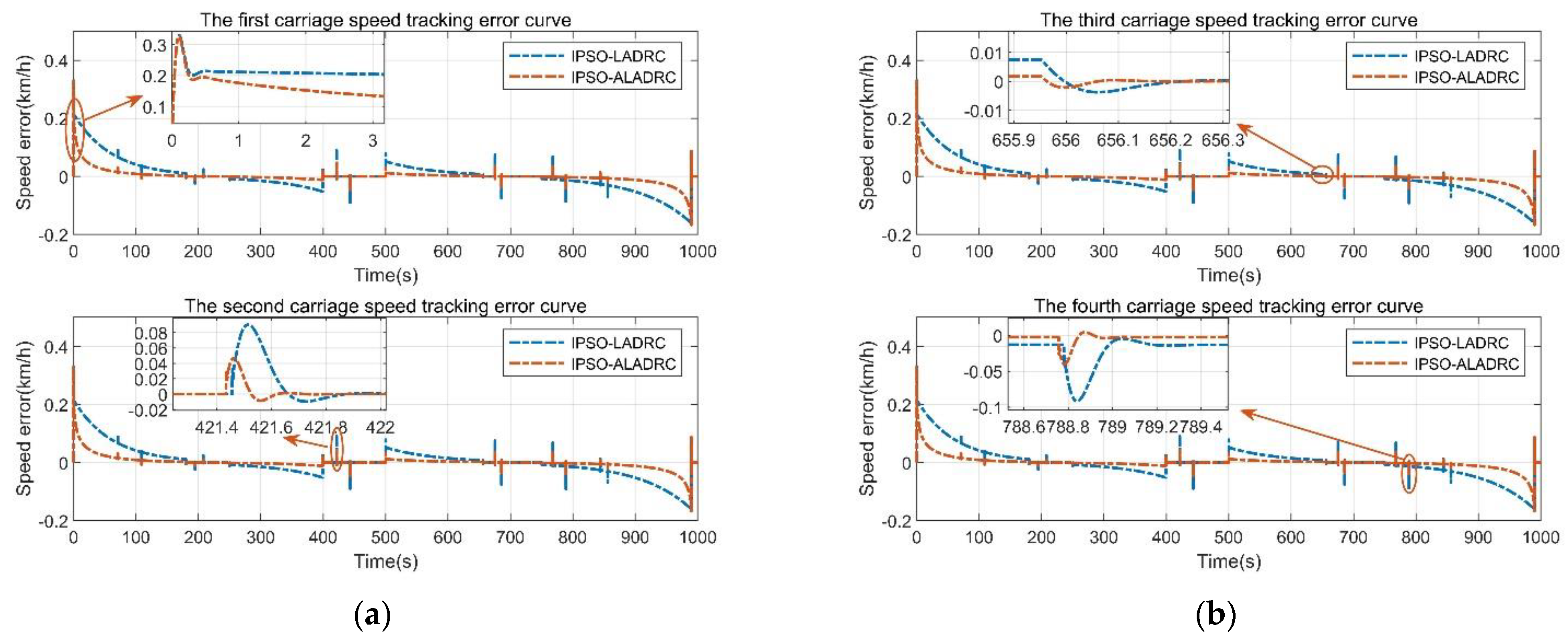
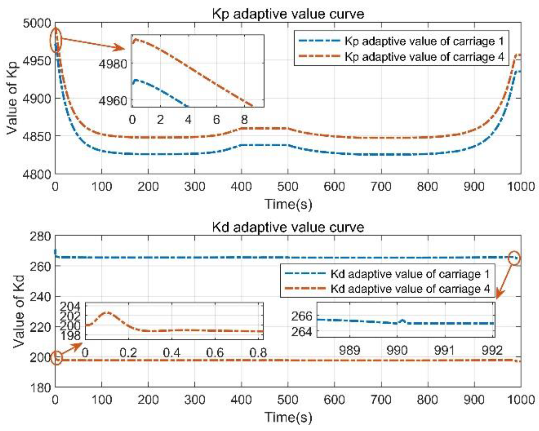
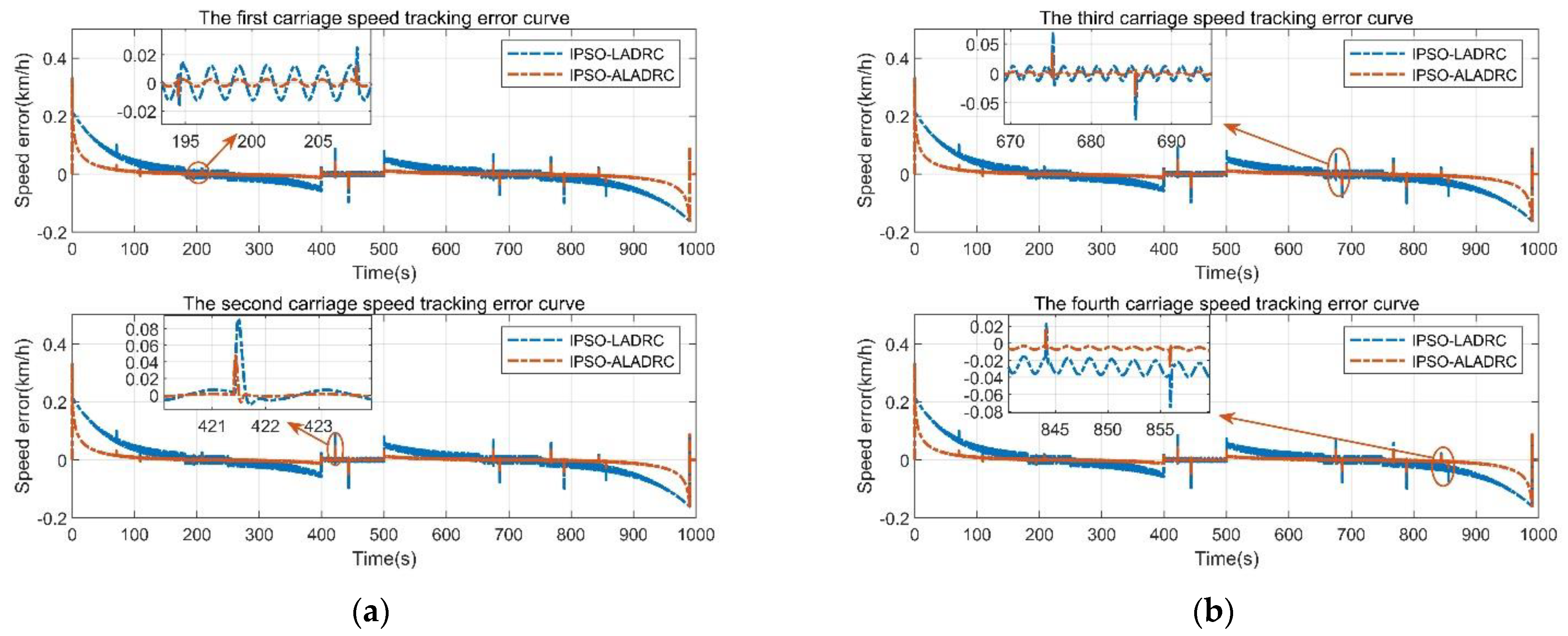
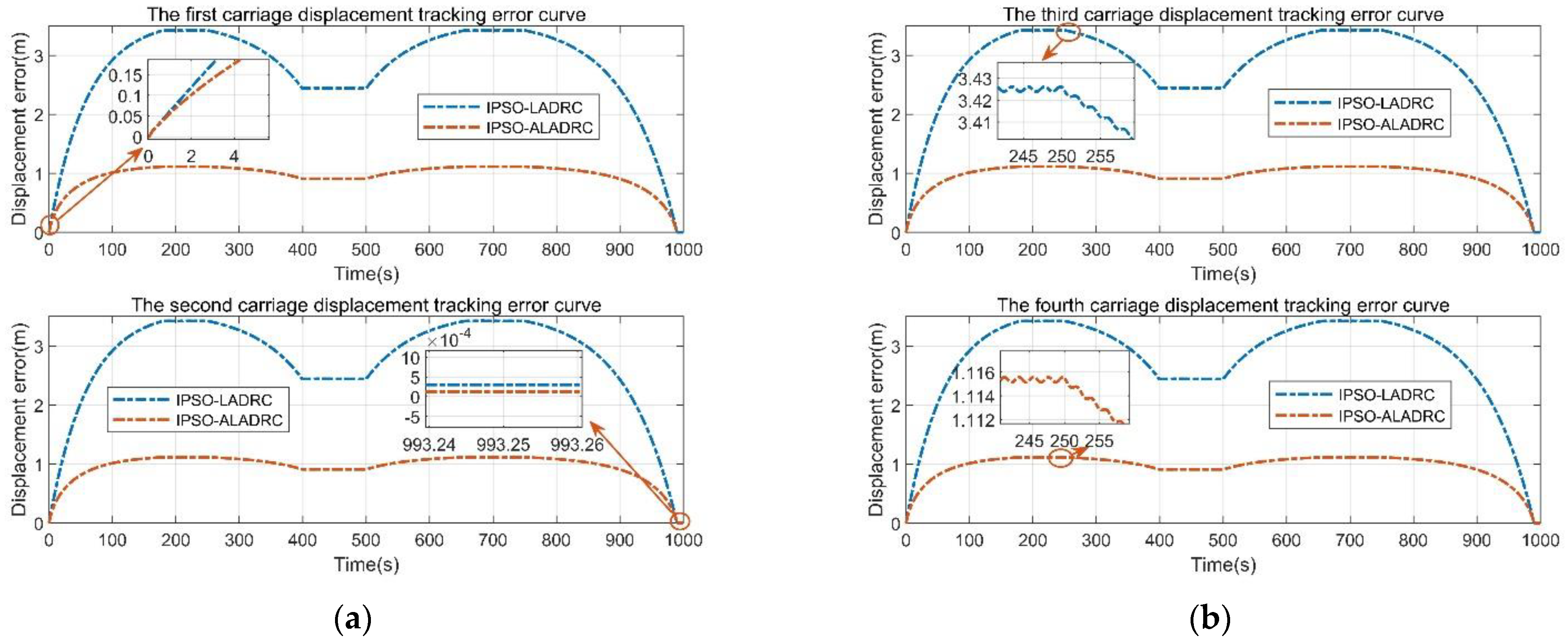
The speed and displacement tracking curves of the four carriages are shown in Figure 7 and Figure 8. It can be seen that both ALADRC and LADRC can make HSTs operate stably according to the ideal speed and displacement curves. When the ideal speed suddenly changes, the speed and displacement tracking errors of both are relatively small. They can meet the requirement that the maximum speed deviation of the train operation does not exceed ± 2   km / h . Compared with LADRC, ALADRC obviously has better control effect. The speed and displacement tracking errors of the four carriages are shown in Figure 9 and Figure 10. It can be seen from Figure 9 that the control performance of ALADRC and LADRC is almost the same at the beginning of the acceleration stage and the final braking stage. However, ALADRC has better control performance during the HST operation. When the HST encounters additional resistance disturbance and a sudden change of the ideal speed signal, ALADRC can suppress the speed fluctuation better and re-track the ideal speed signal in a shorter time. The speed tracking error always exists during HST operation, which will lead to the accumulation of HST displacement error. Therefore, the displacement tracking error of HSTs with ALADRC is significantly smaller than LADRC. However, both controllers have a high parking accuracy. The adaptive values of k p and k d are shown in Figure 11. The results show that parameters k p and k d in LADRC can be adjusted in real-time according to the dynamic characteristics and tracking errors.
Through calculation, the speed mean absolute errors of ALADRC and LADRC are 0.0096   km / h and 0.0271   km / h , respectively. This shows that the control performance of LADRC can be effectively improved by setting adaptive laws for PD controller parameters and LESO. This also proves that ALADRC is more suitable as a HST speed tracking controller.
Example 2. 
This part is used to verify the control performance of ALADRC when HST coefficients change with time.The coefficients of the Davis equation and the mass of the carriage may change during the HST operation, and periodic functions are added to the above coefficients as time-varying perturbations [37]. The details are as follows:  c 0 + r 1 , c v + r 2 , c a + r 3 , and m + r 4 , where r 1 = 0.15 × sin ( t ) , r 2 = 0.0015 × sin ( 2 t ) , r 3 = 0.00015 × sin ( 3 t ) , and r 4 = 0.1 × sin ( 4 t ) . The above time-varying coefficients are shown in Figure 12. The HST operating environment and LADRC parameters are consistent with Example 1.
The speed tracking error of the four carriages is shown in Figure 13. It can be seen that the speed tracking error of the HST fluctuates periodically compared with Example 1. The range of the HST with ALADRC speed fluctuation is ± 0.005   km / h , and the range of LADRC speed fluctuation is ± 0.015   km / h . Therefore, ALADRC is significantly better than LADRC in suppressing the adverse effects of time-varying parameters. The displacement tracking error of the four carriages is shown in Figure 14. It can be seen that due to the periodic change of the HST speed error, its displacement error will also have periodic changes. The error variation range of ALADRC is smaller than LADRC, but neither of them will adversely affect the normal operation of HSTs and will not reduce the parking accuracy of HSTs.
Through calculation, the speed mean absolute errors of ALADRC and LADRC are 0.015   km / h and 0.0315   km / h , respectively. ALADRC also has better control performance than LADRC. In conclusion, the LADRC optimized by IPSO has good control performance. On this basis, the introduction of APC can further improve the control performance of LADRC. Therefore, the control scheme combining IPSO and ALADRC is more suitable for the HST speed tracking controller.

5. Conclusions

This paper proposes a control scheme combining IPSO and ALADRC to solve the HST speed tracking control problem. In the establishment of a HST model, a multi-mass point dynamic model with time-varying coefficients is considered. The running resistance, the additional resistance, the interaction force between carriages, and the time-varying coefficients are taken as disturbances to verify the effectiveness of the designed control scheme. In the design of a control scheme, LADRC is used as the HST speed tracking controller. The LESO can estimate and compensate for the total disturbance in real-time, meaning that each carriage can be independently controlled by LADRC without decoupling. In view of the difficulty in setting the LADRC parameters of different carriages, IPSO is introduced to optimize the LADRC parameters of different carriages according to the optimization objective of minimizing the HST speed tracking error. This greatly simplifies the parameter adjustment process. In order to compensate for the observation error of LESO and further improve the control performance of LADRC when the HST encounters unknown disturbances during actual operation, APC is introduced. From the simulation results, it can be seen that it is feasible to use IPSO to optimize LADRC parameters, and the speed tracking error of the HST is small, which meets the requirements of HST operation. With the introduction of APC, ALADRC has better adaptability than LADRC with fixed parameters in the dynamic control process. From the simulation results of two examples, it can be seen that the HST using ALADRC has stronger anti-disturbance performance, faster response speed, and higher control accuracy when encountering disturbances. The HST speed mean absolute errors of ALADRC are smaller than LADRC. This can prove the effectiveness of the designed control scheme. At present, this paper is limited to theoretical analysis, and some practical problems are not considered, such as the traction and braking characteristics of the train traction motor, the energy demand of the actuator, and the signal transmission mode. These issues will be considered in the next work.

Author Contributions

J.X., contributed to the conception of the study, performed the experiment, performed the data analyses, and wrote the manuscript; K.Z. and T.Z., contributed to the conception of the study; M.Z., Z.Q., S.C. and Y.G., helped perform the analysis with constructive discussions. All authors have read and agreed to the published version of the manuscript.

Funding

The authors received no financial support for the research, authorship, and/or publication of this article.

Institutional Review Board Statement

Not applicable.

Informed Consent Statement

Not applicable.

Data Availability Statement

Not applicable.

Conflicts of Interest

The authors declare that they have no competing interests.

References

  1. Yao, X.; Park, J.; Dong, H.; Guo, L.; Lin, X. Robust adaptive nonsingular terminal sliding mode control for automatic train operation. IEEE Trans. Syst. Man Cybern. Syst. 2018, 49, 2406–2415. [Google Scholar] [CrossRef]
  2. Zhao, C.; Chen, J.; Zhang, X.; Wang, Z.; Wu, P.; Cui, Z. Fluctuating Demand-Oriented Optimization of Train Line Planning Considering Carriage Resources Transfer under Flexible Compositions. Appl. Sci. 2022, 12, 8965. [Google Scholar] [CrossRef]
  3. Li, Z.; Hou, Z.; Yin, C. Iterative learning control for train trajectory tracking under speed constrains with iteration-varying parameter. Trans. Inst. Meas. Control 2015, 37, 485–493. [Google Scholar] [CrossRef]
  4. Mikulski, J.; Gorzelak, K. Conception of modernization of a line section example in the context of a fast railway connection. Arch. Transp. 2017, 44, 47–54. [Google Scholar] [CrossRef] [Green Version]
  5. Chen, X.; Zhang, Y.; Huang, H. Train speed control algorithm based on PID controller and single-neuron PID controller. In Proceedings of the 2010 Second WRI Global Congress on Intelligent Systems, Wuhan, China, 16–17 December 2010; pp. 107–110. [Google Scholar]
  6. Mo, X.; Tang, T.; Dong, C.; Yao, Y.; Yao, X. A realization and simulation of ATO speed control module-predictive fuzzy control algorithm. In Proceedings of the 2013 IEEE International Conference on Intelligent Rail Transportation Proceedings, Beijing, China, 30 August 2013; pp. 263–267. [Google Scholar]
  7. Cao, Y.; Ma, L.; Zhang, Y. Application of fuzzy predictive control technology in automatic train operation. Clust. Comput. 2019, 22, 14135–14144. [Google Scholar] [CrossRef]
  8. Mao, Z.; Yan, X.; Jiang, B.; Chen, M. Adaptive fault-tolerant sliding-mode control for high-speed trains with actuator faults and uncertainties. IEEE Trans. Intell. Transp. Syst. 2020, 21, 2449–2460. [Google Scholar] [CrossRef] [Green Version]
  9. Li, S.; Yang, L.; Gao, Z. Adaptive coordinated control of multiple high-speed trains with input saturation. Nonlinear Dyn. 2016, 83, 2157–2169. [Google Scholar] [CrossRef]
  10. He, Z.; Yang, Z.; Lu, J. Braking control algorithm for accurate train stopping based on adaptive fuzzy sliding mode. China Railw. Sci. 2019, 40, 122–129. [Google Scholar]
  11. Lin, C.; Tsai, S.; Chen, C.; Li, T. Extended sliding-mode controller for high speed train. In Proceedings of the 2010 International Conference on System Science and Engineering, Taipei, Taiwan, 1–3 July 2010; pp. 475–480. [Google Scholar]
  12. Dong, H.; Gao, S.; Ning, B. Cooperative control synthesis and stability analysis of multiple trains under moving signaling systems. IEEE Trans. Intell. Transp. Syst. 2016, 17, 2730–2738. [Google Scholar] [CrossRef]
  13. Wang, B.; Yang, J.; Jiao, H.; Zhu, K.; Chen, Y. Design of auto disturbance rejection controller for train traction control system based on artificial bee colony algorithm. Measurement 2020, 160, 107812. [Google Scholar] [CrossRef]
  14. Kong, X.; Zhang, T. Non-singular fast terminal sliding mode control of high-speed train network system based on improved particle swarm optimization algorithm. Symmetry 2020, 12, 205. [Google Scholar] [CrossRef]
  15. Hou, T.; Guo, Y.; Ni, H. Research on speed control of high-speed train based on multi-point model. Arch. Transp. 2019, 50, 35–46. [Google Scholar] [CrossRef]
  16. Chen, Y.; Huang, D.; Huang, T.; Qin, N. Tracking control via iterative learning for high-speed trains with distributed input constraints. IEEE Access 2019, 7, 84591–84601. [Google Scholar] [CrossRef]
  17. Ji, H.; Hou, Z.; Zhang, R. Adaptive iterative learning control for high-speed trains with unknown speed delays and input saturations. IEEE Trans. Autom. Sci. Eng. 2016, 13, 260–273. [Google Scholar] [CrossRef]
  18. Han, J. Active disturbance rejection controller and application. Control Decis. 1998, 13, 3–5. [Google Scholar]
  19. Gao, Z. Scaling and bandwidth-parameterization based controller tuning. Proc. Am. Control Conf. 2006, 6, 4989–4996. [Google Scholar]
  20. Cheng, M.; Jiao, X. Modified active disturbance rejection control for non-linear semi-active vehicle suspension with magneto-rheological damper. Trans. Inst. Meas. Control 2018, 40, 2611–2621. [Google Scholar] [CrossRef]
  21. Yu, T.; Chan, K.; Tong, J.; Zhou, B.; Li, D. Coordinated robust nonlinear boiler-turbine-generator control systems via approximate dynamic feedback linearization. J. Process Control 2010, 20, 365–374. [Google Scholar] [CrossRef]
  22. Pawar, S.; Chile, R.; Patre, B. Modified reduced order observer based linear active disturbance rejection control for TITO systems. ISA Trans. 2017, 71, 480–494. [Google Scholar] [CrossRef]
  23. Zhou, X.; Zhong, W.; Ma, Y.; Guo, K.; Yin, J.; Wei, C. Control strategy research of D-STATCOM using active disturbance rejection control based on total disturbance error compensation. IEEE Access 2021, 9, 50138–50150. [Google Scholar] [CrossRef]
  24. Zhao, F.; Wang, X.; Zhu, T. Power Dynamic Decoupling Control of Grid-Forming Converter in Stiff Grid. IEEE Trans. Power Electron. 2022, 37, 9073–9088. [Google Scholar] [CrossRef]
  25. Liu, C.; Cheng, Y.; Liu, D.; Cao, G.; Lee, I. Research on a LADRC strategy for trajectory tracking control of delta high-speed parallel robots. Math. Probl. Eng. 2020, 2020, 12. [Google Scholar] [CrossRef]
  26. Hua, L.; Zhang, J.; Li, D.; Xi, X. Fault-Tolerant Active Disturbance Rejection Control of Plant Protection of Unmanned Aerial Vehicles Based on a Spatio-Temporal RBF Neural Network. Appl. Sci. 2021, 11, 4084. [Google Scholar] [CrossRef]
  27. Guo, B.; Bacha, S.; Alamir, M.; Mohamed, A.; Boudinet, C. LADRC applied to variable speed micro-hydro plants: Experimental validation. Control Eng. Pract. 2019, 85, 290–298. [Google Scholar] [CrossRef]
  28. Zhou, Y.; Luo, D.; Wu, B.; Cheng, B.; Lin, Q. Active vibration isolation system based on the LADRC algorithm for atom interferometry. Appl. Opt. 2020, 59, 3487–3493. [Google Scholar] [CrossRef] [PubMed]
  29. Geng, X.; Zhu, Q.; Liu, T.; Na, J. U-model based predictive control for nonlinear processes with input delay. J. Process Control 2019, 75, 156–170. [Google Scholar] [CrossRef] [Green Version]
  30. Wang, H.; Huang, H. Property and applications of extended state observer. Control Decis. 2013, 28, 1078–1082. [Google Scholar]
  31. Liu, Y.; Zhou, Y.; Sun, S.; Xun, J.; Tang, T. An analytical optimal control approach for virtually coupled. Transp. Res. Part C Emerg. Technol. 2020, 125, 102886. [Google Scholar] [CrossRef]
  32. Arnold, M.; Burgermeister, B.; Fuhrer, C.; Hippmann, G.; Rill, G. Numerical methods in vehicle system dynamics: State of the art and current developments. Veh. Syst. Dyn. 2011, 49, 1159–1207. [Google Scholar] [CrossRef]
  33. Chen, B.; Huang, Z.; Zhang, R.; Jiang, F.; Liu, W.; Li, H.; Peng, J. Adaptive slip ratio estimation for active braking control of high-speed trains. ISA Trans. 2021, 112, 302–314. [Google Scholar] [CrossRef]
  34. Chu, H.; Yi, J.; Yang, F. Chaos Particle Swarm Optimization Enhancement Algorithm for UAV Safe Path Planning. Appl. Sci. 2022, 12, 8977. [Google Scholar] [CrossRef]
  35. Wu, L.; Han, J. Active disturbance rejection controller scheme for the linear inverted pendulum. Control Theory Appl. 2004, 21, 665–670. [Google Scholar]
  36. Mou, J.; Zhang, W.; Wu, C.; Guo, Q. Adaptive Control of Flapping-Wing Micro Aerial Vehicle with Coupled Dynamics and Unknown Model Parameters. Appl. Sci. 2022, 12, 9104. [Google Scholar] [CrossRef]
  37. Tang, H.; Wang, Q.; Feng, X. Robust stochastic control for high-speed trains with nonlinearity, parametric uncertainty, and multiple time-varying delays. IEEE Trans. Intell. Transp. Syst. 2018, 19, 1027–1037. [Google Scholar] [CrossRef]
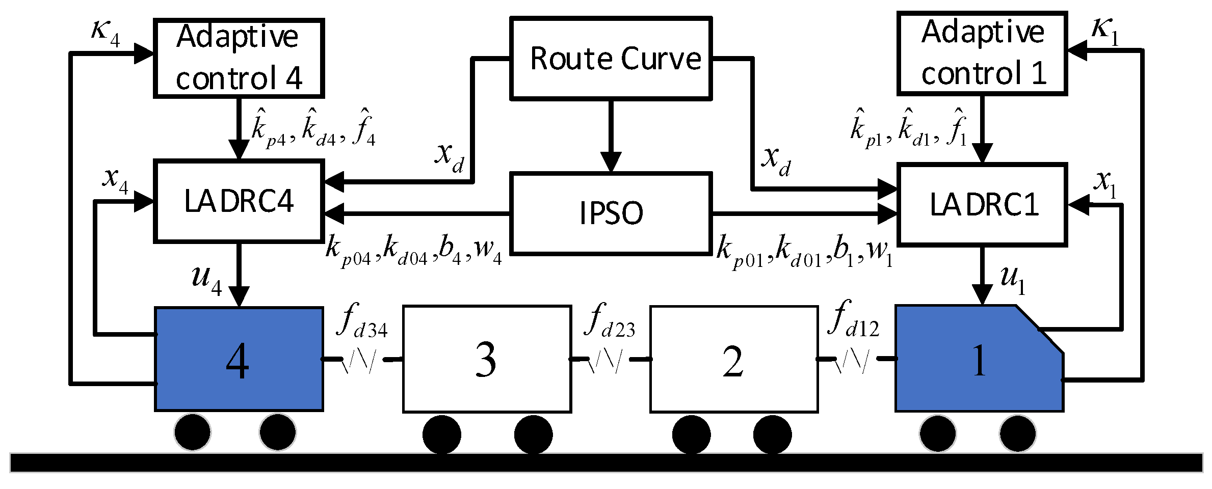
Figure 1. Control scheme structure diagram.
Applsci 12 10558 g001
Figure 2. IPSO algorithm optimization process.
Applsci 12 10558 g002
Figure 3. ALADRC control structure diagram.
Applsci 12 10558 g003
Figure 4. Ideal speed and displacement curve.
Applsci 12 10558 g004
Figure 5. LADRC parameters change curve.
Applsci 12 10558 g005
Figure 6. Objective function value change curve.
Applsci 12 10558 g006
Figure 7. Speed tracking curve of the four carriages: (a) Speed tracking curve of the first two carriages; (b) Speed tracking curve of the last two carriages.
Applsci 12 10558 g007
Figure 8. Displacement tracking curve of the four carriages: (a) Displacement tracking curve of the first two carriages; (b) Displacement tracking curve of the last two carriages.
Applsci 12 10558 g008
Figure 9. Speed tracking error of the four carriages: (a) Speed tracking error of the first two carriages; (b) Speed tracking error of the last two carriages.
Applsci 12 10558 g009
Figure 10. Displacement tracking error of the four carriages: (a) Displacement tracking error of the first two carriages; (b) Displacement tracking error of the last two carriages.
Applsci 12 10558 g010
Figure 11. k p and k d adaptive values.
Applsci 12 10558 g011
Figure 12. Change of time-varying coefficients.
Applsci 12 10558 g012
Figure 13. Speed tracking error of the four carriages: (a) Speed tracking error of the first two carriages; (b) Speed tracking error of the last two carriages.
Applsci 12 10558 g013
Figure 14. Displacement tracking error of the four carriages: (a) Displacement tracking error of the first two carriages; (b) Displacement tracking error of the last two carriages.
Applsci 12 10558 g014
Table 1. Ramp, curve, and tunnel road parameters.
Road ConditionParameter Setting Starting   ( m ) Ending   ( m )
Ramp θ 1 = 10 0 00 3000 6000
θ 2 = 8 0 00 14 , 000 15 , 300
Curve R 1 = 10 , 000   m 34 , 000 35 , 500
R 2 = 12 , 000   m 55 , 000 56 , 000
Tunnel L 1 = 2000   m 64 , 000 66 , 000
L 2 = 1000   m 71 , 000 72 , 000
Table 2. Parameters of the HST.
ParametersValue
Mass   of   sin gle   carriage   m   ( t ) 47.5
Davis   equation   f a   ( N / KN ) 7.75 + 0.0228   v + 0.00166   v 2
Hook   damping   coupling   k   ( N / m ) 2 × 10 7
Hook   elastic   coupling   d   ( N s / m ) 5 × 10 6
Table 3. Controller parameters of ALADRC and LADRC.
Parameters k p 0 k d 0 w b
First carriage 4969 268 200 0.111
Fourth carriage 4991 200 200 0.113
Publisher’s Note: MDPI stays neutral with regard to jurisdictional claims in published maps and institutional affiliations.